OMI NO<sub>2</sub> column densities over North American urban cities: the effect of satellite footprint resolution

(1)

GMDD

8, 8451–8479, 2015

OMI NO2 column

densities over North American urban

cities

H. C. Kim et al.

Title Page

Abstract Introduction

Conclusions References

Tables Figures

◭ ◮

Back Close

Full Screen / Esc

Printer-friendly Version

Interactive Discussion

Discussion

P

a

per

|

Discussion

P

a

per

|

Discussion

P

a

per

|

Discussion

P

a

per

|

Geosci. Model Dev. Discuss., 8, 8451–8479, 2015 www.geosci-model-dev-discuss.net/8/8451/2015/ doi:10.5194/gmdd-8-8451-2015

This discussion paper is/has been under review for the journal Geoscientific Model Development (GMD). Please refer to the corresponding final paper in GMD if available.

OMI NO

₂

column densities over North

American urban cities: the e

_ff

ect of

satellite footprint resolution

H. C. Kim1,2, P. Lee1, L. Judd3, L. Pan1,2, and B. Lefer3

1

NOAA/Air Resources Laboratory, College Park, MD, USA

2

UMD/Cooperative Institute for Climate and Satellites, College Park, MD, USA

3

University of Houston, Houston, TX, USA

Received: 31 August 2015 – Accepted: 2 September 2015 – Published: 2 October 2015

Correspondence to: H. C. Kim ([email protected])

(2)

GMDD

8, 8451–8479, 2015

cities

H. C. Kim et al.

Title Page

Tables Figures

◭ ◮

Back Close

Full Screen / Esc

Discussion

P

a

per

|

Discussion

P

a

per

|

Discussion

P

a

per

|

Discussion

P

a

per

|

Abstract

Nitrogen dioxide vertical column density (NO2 VCD) measurements via satellite are

compared with a fine-scale regional chemistry transport model, using a new approach that considers varying satellite footprint sizes. Space-borne NO₂ VCD measurement has been used as a proxy for surface nitrogen oxide (NO_x) emission, especially for

an-5

thropogenic urban emission, so accurate comparison of satellite and modeled NO2

VCD is important in determining the future direction of NO_x emission policy. The National Aeronautics and Space Administration Ozone Monitoring Instrument (OMI) NO2 VCD measurements, retrieved by the Royal Netherlands Meteorological Institute

(KNMI), are compared with a 12 km Community Multi-scale Air Quality (CMAQ)

simu-10

lation from the National Oceanic and Atmospheric Administration. We found that OMI footprint pixel sizes are too coarse to resolve urban NO2plumes, resulting in a

possi-ble underestimation in the urban core and overestimation outside. In order to quantify this effect of resolution geometry, we have made two estimates. First, we constructed pseudo-OMI data using scale outputs of the model simulation. Assuming the

fine-15

scale model output is a true measurement, we then collected real OMI footprint cover-ages and performed conservative spatial regridding to generate a set of fake OMI pixels out of fine-scale model outputs. When compared to the original data, the pseudo-OMI data clearly showed smoothed signals over urban locations, resulting in roughly 20– 30 % underestimation over major cities. Second, we further conducted conservative

20

downscaling of OMI NO2 VCD using spatial information from the fine-scale model to

adjust the spatial distribution, and also applied Averaging Kernel (AK) information to adjust the vertical structure. Four-way comparisons were conducted between OMI with and without downscaling and CMAQ with and without AK information. Results show that OMI and CMAQ NO₂ VCDs show the best agreement when both downscaling

25

(3)

GMDD

8, 8451–8479, 2015

cities

H. C. Kim et al.

Title Page

Tables Figures

◭ ◮

Back Close

Full Screen / Esc

Discussion

P

a

per

|

Discussion

P

a

per

|

Discussion

P

a

per

|

Discussion

P

a

per

|

considered when using satellite observations in emission policy making, and the new downscaling approach can provide a reference uncertainty for the use of satellite NO₂ measurements over most cities.

1 Introduction

Tropospheric nitrogen dioxide, NO₂, is an important component of urban atmospheric

5

chemistry. It is one of the major pollutants affecting humans and the biosphere (Chauhan et al., 2003; Kampa and Castanas, 2008), and works as an important pre-cursor in tropospheric ozone chemistry and aerosol formation. Continuous monitor-ing of tropospheric NO2 is important to understand urban air quality and changes in

anthropogenic emissions. NO2 is also used as an important indicator for traffic and 10

urbanization (Rijnders et al., 2001; Ross et al., 2006; Studinicka et al., 1997).

Tropospheric NO2 has been measured from space since the mid-1990s; the Global

Ozone Monitoring Experiment (GOME, 1996–2003, onboard the European Remote Sensing-2), Scanning Imaging Absorption SpectroMeter for Atmospheric CHartog-raphY (SCIAMACHY, 2002–2012, onboard ENVISAT), Ozone Monitoring Instrument

15

(OMI, 2004–present, onboard Aura), and GOME-2 (2007–present, onboard MetOp-A and 2013–present on MetOp-B) have all been used for the detection of NO_x emis-sion from natural and anthropogenic sources (Beirle et al., 2004; Boersma et al., 2007; Kim et al., 2006, 2009; Konovalov et al., 2006; Lamsal et al., 2008; Martin et al., 2003; Napelenok et al., 2008; Richter et al., 2005; van der A et al., 2006, 2008)

20

NO₂ plumes from urban anthropogenic sources, especially from point and mobile sources, usually have a fine structure, as small as a few hundred meters and as large as 10–20 km, as reported in comparisons of column NO2based on in situ observations

and modeled calculations (Heue et al., 2008; Valin et al., 2011; Ryerson et al., 2001). Heue et al. (2008) used an airborne instrument based on imaging Differential Optical

25

(4)

GMDD

8, 8451–8479, 2015

cities

H. C. Kim et al.

Title Page

Tables Figures

◭ ◮

Back Close

Full Screen / Esc

Discussion

P

a

per

|

Discussion

P

a

per

|

Discussion

P

a

per

|

Discussion

P

a

per

|

Highveld with OMI and SCIAMACHY measurements, they demonstrated that iDOAS shows strong enhancements close to industrial areas, 4–9 times higher than measure-ments from OMI and SCIAMACHY. Previous studies have demonstrated that modeled ozone production depends strongly on the spatial scale of the modeling grid due to the nonlinear dependence of ozone production on NOx concentration (e.g., Cohan et al., 5

2006; Gillani and Pleim, 1996; Liang and Jacobson, 2000; Sillman et al., 1990), so an accurate comparison of urban NO₂ plumes in fine scale is crucial for understanding surface ozone chemistry and air pollution over urban cities. Using 1-D and 2-D models, Valin et al. (2011) computed the resolution-dependent bias in the predicted NO2

col-umn, demonstrating large negative biases over large sources and positive biases over

10

small sources at coarse model resolution.

The inhomogeneity of urban NO2plumes within the scale of satellite footprint pixels is

of rising interest as satellite-based measurements are being compared with fine-scale modeling (Beirle et al., 2004, 2011; Hilboll et al., 2013). Richter et al. (2005) showed that there are considerable differences between GOME and SCIAMACHY observations

15

for locations with steep gradients in the tropospheric NO2columns, while these

obser-vations agree very well over large areas of relatively homogeneous NO₂signals. Hilboll et al. (2013) argued that these effects result from spatial smoothing that differs depend-ing on the ground resolution of the instruments, so the inherent spatial heterogeneity of the NO_x fields must be considered when studying them over small, localized areas.

20

Hilboll et al. (2013) also presented approaches to account for instrumental differences while preserving individual instruments’ spatial resolutions. In comparing GOME and SCIAMACHY, they used an explicit climatological correction factor to convolve GOME pixels (40 km×320 km) with better-resolution SCIAMACHY (30 km×60 km) data, pro-ducing a combined data set for studying long-term trends.

25

In this study, we try to investigate and to quantify the uncertainty resulting from the geometry of OMI satellite-based NO2 VCD measurements by comparing these data

(5)

GMDD

8, 8451–8479, 2015

cities

H. C. Kim et al.

Title Page

Tables Figures

◭ ◮

Back Close

Full Screen / Esc

Discussion

P

a

per

|

Discussion

P

a

per

|

Discussion

P

a

per

|

Discussion

P

a

per

|

data in order to quantify the impact from pure differences in geometry. Second, we extend the basic concept of Hilboll et al. (2013) to apply spatial-distribution informa-tion from the fine-scale model to the OMI measurements, and demonstrate how the new approach adjusts the original OMI measurements. Satellite and model data are described in Sect. 2. Construction of pseudo-OMI data and the quantification of the

im-5

pact of pixel geometry are discussed in Sect. 3. In Sect. 4, the downscaling approach is discussed; Sect. 5 concludes and discusses the implications of findings for emission policy decision-making.

2 Data

OMI: We utilized OMI tropospheric NO₂VCD data, retrieved by the Royal Netherlands

10

Meteorological Institute (KNMI). The OMI instrument, onboard NASA’s Earth Observ-ing System Aura satellite, is a nadir-viewObserv-ing imagObserv-ing spectrograph measurObserv-ing backscat-tered solar radiation with a measuring wavelength ranging from 270 to 500 nm and with a spectral resolution of about 0.5 nm. Its telescope has a 114◦ viewing angle, which corresponds to a 2600 km-wide swath on the surface. In its normal global

oper-15

ation mode, its pixel size is 13 km (along)×24 km (across) at nadir, which can be re-duced to 13 km×12 km in zoom mode (Levelt et al., 2006). Data were downloaded from the European Space Agency’s (ESA) Tropospheric Emission Monitoring Internet Ser-vice (TEMIS; http://www.temis.nl/airpollution/no2.html). DOMINO version 2.0 retrieval based on the Differential Optical Absorption Spectroscopy (DOAS) technique was used

20

for the study. We disregarded data pixels with cloud fractions over 40 % or other con-taminated pixels using quality flags. Details on the NO2column retrieval algorithms and

error analysis are described in Boersma et al. (2004, 2007).

NAQFC: The US National Air Quality Forecast Capability (NAQFC) provides daily, ground-level ozone predictions using the Weather Forecasting and Research

non-25

(6)

analy-GMDD

8, 8451–8479, 2015

cities

H. C. Kim et al.

Title Page

Tables Figures

◭ ◮

Back Close

Full Screen / Esc

Discussion

P

a

per

|

Discussion

P

a

per

|

Discussion

P

a

per

|

Discussion

P

a

per

|

sis, we used the experimental version of NAQFC, which uses WRF-NMM with B-grid (NMMB) as a meteorological driver and the CB05 chemical mechanism. Meteorological data is processed using the PREMAQ, which is a special version of the Meteorology– Chemistry Interface Processor (MCIP) designed for the NAQFC system.

3 Construction of pseudo-OMI data 5

OMI footprint pixel size increases as the viewing angle deviates from the nadir direction to the edge of swaths. Figure 1 shows the actual size distributions of OMI pixels col-lected during September 2013. The blue line indicates size distribution counts for each 50 km2bin, while the red line indicates the cumulative distribution of the OMI pixel sizes. The size distribution has high occurrences near 300 km2, as expected from the OMI’s

10

resolution at the nadir (that is, 13×24=312). However, many pixels still have larger sizes; around half of total pixels are larger than 500 km2, and 20 % of total pixels are larger even than 1000 km2. Geographical coverage rapidly increases with pixel size, so deciding a threshold for footprint pixel sizes and available coverage may present a serious dilemma.

15

Figure 2 shows the relationship between OMI footprint pixel size and actual geo-graphical coverage over the Contiguous United States (CONUS). With 1 July 2011 data, 25 % of OMI pixel sizes are less than 342 km2, and they cover 1.4 % of the CONUS domain. CONUS coverage changes to 11.5, 24.0, and 58.8 % when 50, 75, and 100 % of OMI pixels are used, respectively. Using only finer data may provide

de-20

tailed information, but they represent only a small part of all the data. If we also use coarser-resolution data, they provide more coverage but tend to be biased over areas with spatial gradient, as discussed in the previously mentioned studies (Hilboll et al., 2013). We therefore estimated the theoretical range of biases deriving from this geo-metric effect by constructing a pseudo-OMI data set out of a fine-scale model. Using

25

(7)

GMDD

8, 8451–8479, 2015

cities

H. C. Kim et al.

Title Page

Tables Figures

◭ ◮

Back Close

Full Screen / Esc

Discussion

P

a

per

|

Discussion

P

a

per

|

Discussion

P

a

per

|

Discussion

P

a

per

|

world, we constructed a dataset to mimic OMI instrument measurement of this modeled world.

In order to construct the pseudo-OMI data, we utilized a conservative spatial regrid-ding technique to perform a lossless conversion of gridded modeling outputs into actual OMI footprint pixels. Figure 3 demonstrates the concepts of conservative regridding.

5

The gray grid cells are 12 km grid cells for modeling – zoomed on the Houston region as an example – and the blue lines are actual OMI pixel coverage. The blue, shaped pixel is an example of an actual OMI pixel, while the pink boxes are model grid cells overlaid by the example OMI pixel. The numbers in the grid cells are calculations of the fractional area overlaid by the OMI pixel for each cell using the Sutherland–Hodman

10

polygon-clipping algorithms available from the IDL-based Geospatial Data Processor (Kim et al., 2013); 0.74 means the OMI pixel covers 74 % of the corresponding grid cell. The pseudo-OMI value for the blue OMI pixel area in Fig. 3 can be estimated as:

P_j =

P

(p_i·fi,j)

P fi,j

(1)

wherei and j are indices for the model grid cell and OMI pixel, respectively. fi,j indi-15

cates the fractional area of celli overlaid by OMI pixelj.

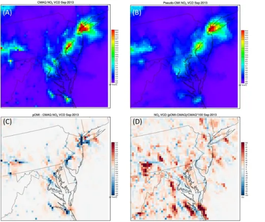
Figure 4 compares the spatial distributions of CMAQ NO₂VCD (assumed to be a true world) and pseudo-OMI (pOMI) NO2VCD, along with the difference and percentage

dif-ference, (pOMI-CMAQ)/CMAQ×100, over the northeastern United States. It is evident that there are prominent differences between the original fine-scale modeled NO₂VCD

20

and reconstructed pseudo-OMI distribution, especially over and near urban locations. As expected from the smoothing effects of larger pixel sizes, pOMI shows a slightly smoothed transition from urban cores to suburban, and most of the sharp peaks near small cities are gone in the pOMI distribution. As already mentioned, this is purely a result of geometry. We can see that, for all the major cities, pOMI underestimates

25

the actual NO2VCD values while overestimating at the boundaries of major cities, as

(8)

GMDD

8, 8451–8479, 2015

cities

H. C. Kim et al.

Title Page

Tables Figures

◭ ◮

Back Close

Full Screen / Esc

Discussion

P

a

per

|

Discussion

P

a

per

|

Discussion

P

a

per

|

Discussion

P

a

per

|

areas. This effect is also prominent in locations with small but strong NO_x emission sources, such as power plants or small cities such as Norfolk, VA. It should be noted that these discrepancies result from purely geometric effects deriving from OMI’s de-signed pixel sizes and are around±5–10×1015# cm−2, with 20–30 % underestimation or overestimation biases for major cities and more than 100 % under- or overestimation

5

for local cities like Norfolk and Richmond, VA. In the next section, we introduce a new approach – the conservative downscaling method – to reduce this effect of resolution due to varying OMI footprint pixel sizes.

4 OMI NO2VCD downscaling

As described in the previous section, urban NO₂plumes usually have too fine of a

spa-10

tial structure compared to OMI’s measuring footprints. In this section, we introduce a new approach for adjusting those geometric effects. Downscaling is a common con-cept in meteorological simulations, used especially in global circulation models to pro-vide initial and boundary conditions for regional models. We use a similar concept, describing a downscaling method in data processing as a special case of spatial

re-15

gridding that provides further details through the incorporation of additional information into a set of coarse-resolution data. This approach differs from simply increasing the resolution, as the raw, coarse data are restructured using a set of logics, analogous to a regional meteorological model that downscales global meteorology using its own set of physical and thermal field balances. Conceptually, we use a calculation process

20

reversed from that used to construct the pseudo-OMI data set.

Figure 5 graphically depicts the steps of conservative downscaling from OMI pix-els. Figure 5a shows actual OMI NO₂ VCD measurements over Los Angeles on 4 May 2010, and Fig. 5b shows the corresponding CMAQ NO2 VCD calculated

from NAQFC modeling outputs at the same time and location. As readers can

eas-25

(9)

GMDD

8, 8451–8479, 2015

cities

H. C. Kim et al.

Title Page

Tables Figures

◭ ◮

Back Close

Full Screen / Esc

Discussion

P

a

per

|

Discussion

P

a

per

|

Discussion

P

a

per

|

Discussion

P

a

per

|

cells, as demonstrated in Fig. 5b (black box representing the OMI pixel). We collected those CMAQ pixel values and then normalized them so that the total value of each grid cell sums to one. We call this a spatial-weighting kernel (Fig. 5c), and we ap-ply this weighting kernel to the original OMI measurement. As a result, we generate a reconstructed OMI pixel with finer structure but without any loss of original quantity.

5

Summing the reconstructed pixels gives the original OMI pixel measurement. It should be noted that we strictly apply this method conservatively; theoretically, if there are no missing or duplicated pixels, the quantity of the original data is numerically preserved. This method can be summarized as fusing a satellite-measured “quantity” with mod-eled “spatial information”; the strength of the modmod-eled NO₂ field does not at all affect

10

the result.

As expected, the accuracy of this method indeed depends on the model’s perfor-mance, especially regarding its wind-field simulation and inputs of emission source lo-cations. Considering the uncertainties resulting from emission source locations, the air-quality community has had an excellent archive of geographical information about the

15

geophysical locations of emission sources thanks to the efforts of US EPA, although the strengths of these sources are somewhat highly uncertain. As just described, however, the downscaling method is not affected by emission strength, so we do not think that the uncertainty associated with emission is very high. Wind field is important for simu-lating NO₂ plume transport. With the short lifetime of NO₂, especially during summer,

20

the spatial distribution of NO2 plumes is strongly determined by the location of

emis-sion sources. Improving information about emisemis-sion-source locations would somewhat improve the model, but it is more important to note that the downscaling method tends to convert the error characteristics. Near urban cores, OMI’s coarse footprint resolu-tion always causes unidirecresolu-tional, systematic biases, with underestimaresolu-tion near urban

25

(10)

GMDD

8, 8451–8479, 2015

cities

H. C. Kim et al.

Title Page

Tables Figures

◭ ◮

Back Close

Full Screen / Esc

Discussion

P

a

per

|

Discussion

P

a

per

|

Discussion

P

a

per

|

Discussion

P

a

per

|

4.1 2010 CalNex campaign case

We applied the downscaling technique to compare OMI and downscaled OMI with aircraft-borne measurements from the California Research at the Nexus of Air Quality and Climate (CalNex) campaign. The CalNex field study was conducted in Califor-nia from May to July 2010 and focused on atmospheric-pollution and climate-change

5

issues, including an emission inventory, atmospheric transport and dispersion, atmo-spheric chemical processing, cloud–aerosol interaction, and aerosol radiative effects (Ryerson et al., 2013). Here, we compared NO2 VCD observations from the

cam-paign’s P3 flight with corresponding OMI measurements using both the standard and downscaling methods. More detailed descriptions regarding data preparation and a

dis-10

cussion of the influence of environmental inhomogeneity and urban NO2 plumes are

provided by Judd et al. (2015).

Figure 6 shows scatter-plot comparisons between the P3 measurements and OMI NASA standard product (Fig. 6a), OMI KNMI product (Fig. 6b), and OMI KNMI down-scaled (Fig. 6c) for three days: 4, 7, and 16 May 2010. As reported, the OMI NO2 15

VCD tends to underestimate near the Los Angeles urban area. The KNMI retrieval showed a slightly better comparison with slope=0.73 and R=0.85, while the down-scaled product clearly showed the best agreement with the P3 measurements,R=0.88 and slope=1.0. Deviations still remain from a true one-to-one line even with the down-scaling method; these are possibly caused by errors in wind field simulation. We expect

20

these random errors to average out as the amount of available data increases. The downscaling method seems to work even with daily time-scale data sets.

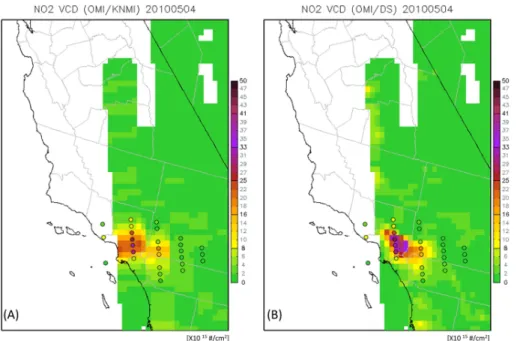
Figure 7 compares OMI NO2 VCD spatial distributions for the original KNMI

prod-ucts with downscaled prodprod-ucts for 4 May 2010, the day when the downscaling method gave the most dramatic changes in the spatial distribution. In the original retrieval, OMI

25

(11)

GMDD

8, 8451–8479, 2015

cities

H. C. Kim et al.

Title Page

Tables Figures

◭ ◮

Back Close

Full Screen / Esc

Discussion

P

a

per

|

Discussion

P

a

per

|

Discussion

P

a

per

|

Discussion

P

a

per

|

very well with the P3 aircraft measurements. On 7 May (not shown), the downscaling method reproduced several peak values very well but failed to generate a clean spot at the edge of Los Angeles. For 16 May (not shown), the changes from downscaling are not dramatic due to generally low NO₂concentrations, but the downscaling method still showed slight enhancement.

5

4.2 Comparison with NAQFC

Comparing modeled NO2 VCD to satellite-observed NO2 VCD has been a popular

way to evaluate the NO_x emission inventory. Since modeled NO₂ VCD and satellite NO2 VCD have different optical and vertical properties, some researchers have used

additional processing to fairly compare satellite and modeled column densities. In this

10

section, we performed vertical and spatial adjustment by applying Averaging Kernel (AK) information in conjunction with the downscaling technique. First, we compared NAQFC NO2VCD with and without AK to OMI NO2VCD with and without downscaling

processing.

The sensitivity of the instrument to tropospheric tracer density is highly

height-15

dependent. Since the measured tracer profile may have large systematic errors as a result, the retrieved tracer columns should be interpreted with proper additional infor-mation (Eskes and Boersma, 2003). An AK stores an instrument’s relative sensitivity to the abundance of the target species for each layer throughout the atmospheric column (Bucsela et al., 2008) and can be applied to a modeled atmospheric column for a fair

20

comparison with satellite retrievals. For each OMI DOMINO product pixel, 34 layers of AKs are provided. We first converted total AK to tropospheric AK, AKtrop, by applying

the total air mass factor (AMF) and tropospheric AMF, and we then applied AKtrop to

model layers before vertically integrating, as described by Herron-Thorpe et al. (2010). When multiple OMI pixels overlaid a model grid cell, we conducted the conservative

25

spatial remapping method explained above.

(12)

GMDD

8, 8451–8479, 2015

cities

H. C. Kim et al.

Title Page

Tables Figures

◭ ◮

Back Close

Full Screen / Esc

Discussion

P

a

per

|

Discussion

P

a

per

|

Discussion

P

a

per

|

Discussion

P

a

per

|

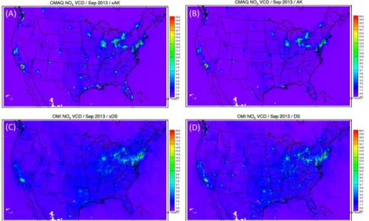
downscaling (Fig. 8c and d, respectively). In general, AK-applied CMAQ NO₂ VCD tends to be slightly lower than CMAQ NO2 VCD without AK information. On the other

hand, while OMI NO2VCD without DS shows a much smoother pattern, the DS-applied

OMI reconstructs the sharp spatial structures near urban areas. DS-applied OMI NO₂ VCD is evidently able to construct sharp gradients near cities, and especially near

5

middle-size cities.

Figure 9 compares CMAQ and OMI NO₂VCDs using AK and DS methods together. Figure 9a shows a scatter-plot comparison between CMAQ and OMI NO2VCDs at US

Environmental Protection Agency Air Quality System (AQS) surface-monitoring site locations. In this comparison, CMAQ NO₂ VCDs are much higher compared to OMI

10

NO₂VCDs, implying that the CMAQ simulation possibly overestimates NO_xemissions. Figure 9c compares OMI and CMAQ NO2VCD with AK information applied; estimated

CMAQ NO2VCD is reduced, showing better agreement with OMI NO2 VCD. Readers

may notice that high CMAQ pixels are shifted to the left. On the other hand, applying the DS method to OMI shifts OMI pixels vertically (Fig. 9b). Finally, in Fig. 9d, both AK and

15

DS methods are applied; this comparison shows the best agreement between OMI and CMAQ NO₂ VCD pixels. Its correlation coe_fficientR=0.89 and the slope of line fit is 0.59. Clearly, the application of the AK and DS methods not only improved the satellite-model comparison in the high NO2concentration range but also significantly improved

the comparison in the low NO₂range (i.e., 0–10×1015molecules cm−2), implying that

20

this method can help interpret NOxemission in major and mid-size cities.

The differences in spatial distributions between monthly averaged OMI and CMAQ NO₂VCDs during September 2013 are shown in Fig. 10. Positive values indicate that CMAQ NO2 VCD is higher than OMI VCD, which should likely be interpreted as an

overestimation of the NO_x emission inventory used in the CMAQ modeling. The

dif-25

(13)

GMDD

8, 8451–8479, 2015

cities

H. C. Kim et al.

Title Page

Tables Figures

◭ ◮

Back Close

Full Screen / Esc

Discussion

P

a

per

|

Discussion

P

a

per

|

Discussion

P

a

per

|

Discussion

P

a

per

|

York, Philadelphia, Detroit, and Chicago – as is expected from the continuous trend of NOx emission reduction, but they are much weaker than in the original

compari-son. Slight overestimations over Baltimore, Washington D.C., Richmond, and Norfolk have almost disappeared. We also notice considerable underestimation of NO₂ VCD over Pennsylvania and West Virginia, which seems to be an impact of recent shale-gas

5

development (e.g., the Marcellus Shale Play) (Chang et al., 2015) that has not been included in the current NAQFC emission-source inventory. Another interesting feature is that there are spots of underestimation over small cities or local power plants; we therefore suspect the DS method slightly overweights urban emissions due to the lack of soil NO_x emissions in the current modeling system.

10

5 Conclusions

This study reports that satellite footprint sizes might cause a considerable effect on the measurement of fine-scale urban NO₂ plumes. Comparing OMI NO₂ VCDs over North American urban cities to a 12 km CMAQ simulation from NOAA NAQFC, we found that OMI footprint-pixel sizes are too coarse to resolve urban plumes, resulting

15

in possible underestimation (and overestimation of model NO₂ VCD) over the urban core and overestimation outside. In order to quantify this effect of resolution, we first conducted a perfect-model experiment. Pseudo-OMI data were constructed using fine-scale outputs of a model simulation, assuming that the fine-fine-scale model output is a true measurement. To match the footprint coverage from real OMI pathways, we conducted

20

conservative spatial regridding with the corresponding fine-scale model outputs to gen-erate a set of pseudo OMI pixels.

When compared to the original data, the pseudo-OMI data clearly showed smoothed signals over urban locations, with 20–30 % underestimation over major cities and up to 100 % bias over smaller urban areas. We then introduced conservative

downscal-25

(14)

ver-GMDD

8, 8451–8479, 2015

cities

H. C. Kim et al.

Title Page

Tables Figures

◭ ◮

Back Close

Full Screen / Esc

Discussion

P

a

per

|

Discussion

P

a

per

|

Discussion

P

a

per

|

Discussion

P

a

per

|

tical structure. Four-way comparisons were conducted between OMI with and without downscaling and CMAQ with and without AK information. Results show that OMI and CMAQ NO2VCDs show the best agreement when both downscaling and AK methods

are applied, with correlation coefficientR=0.89.

These results should be considered when using satellite data in the evaluation of

5

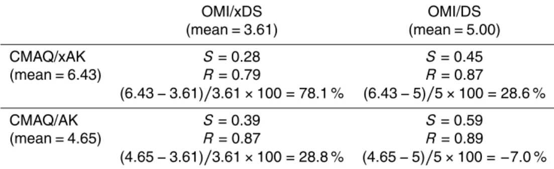
emission inventories and translating these data into decision-making around emission policy. Table 1 shows a summary of the comparisons between OMI and CMAQ NO₂ VCDs described in Figs. 8 and 9. When CMAQ without AK and OMI with DS are com-pared, the percentage difference is (6.43−3.61)/3.61×100=78 %, implying that the current emission inventory likely overestimates NO₂ VCD. Comparing between OMI

10

with DS and CMAQ without AK or between OMI without DS and CMAQ with AK still implies that the current emission inventory is possibly overestimating. However, when both vertical and spatial profiles are adjusted using the AK and DS methods, a slight underestimation is found,−7 %, in modeled NO2VCD over AQS monitoring locations,

implying that the current inventory possibly underestimates emissions. This may

rep-15

resent an important implication for how spatial information should be considered when investigating fine-scale phenomena such as urban NO₂plumes.

Without question, satellite observations are very useful with their large coverage sup-plementing sparse surface-monitoring sites. Interpretation of satellite-based measure-ment, however, should be performed cautiously with consideration of the instrument’s

20

characteristics, especially when translating results into policy-making. We expect our current study to provide a reference for the uncertainty of satellite-based information regarding local or regional pollutants, especially until we have the measurement data at more enhanced resolution that will be provided by future satellites, such as TEMPO, TROPOMI, and GEMS.

25

(15)

GMDD

8, 8451–8479, 2015

cities

H. C. Kim et al.

Title Page

Tables Figures

◭ ◮

Back Close

Full Screen / Esc

Discussion

P

a

per

|

Discussion

P

a

per

|

Discussion

P

a

per

|

Discussion

P

a

per

|

References

Beirle, S., Platt, U., Wenig, M., and Wagner, T.: Highly resolved global distribution of tropo-spheric NO₂ using GOME narrow swath mode data, Atmos. Chem. Phys., 4, 1913–1924, doi:10.5194/acp-4-1913-2004, 2004.

Beirle, Steffen, Boersma, K. F., Platt, U., Lawrence, M. G., and Wagner, T.: Megacity

emis-5

sions and lifetimes of nitrogen oxides probed from space, Science, 333, 1737–1739, doi:10.1126/science.1207824, 2011.

Boersma, K. F., Eskes, H. J., and Brinksma, E. J.: Error analysis for tropospheric NO₂retrieval from space, J. Geophys. Res., 109, D04311, doi:10.1029/2003JD003962, 2004.

Boersma, K. F., Eskes, H. J., Veefkind, J. P., Brinksma, E. J., van der A, R. J., Sneep, M.,

10

van den Oord, G. H. J., Levelt, P. F., Stammes, P., Gleason, J. F., and Bucsela, E. J.: Near-real time retrieval of tropospheric NO₂from OMI, Atmos. Chem. Phys., 7, 2103–2118, doi:10.5194/acp-7-2103-2007, 2007.

Bucsela, E. J., Perring, A. E., Cohen, R. C., Boersma, K. F., Celarier, E. A., Gleason, J. F., and Veefkind, J. P.: Comparison of tropospheric NO₂ from in situ aircraft measurements

15

with near-real-time and standard product data from OMI, J. Geophys. Res., 113, D16S31, doi:10.1029/2007JD008838, 2008.

Chai, T., Kim, H.-C., Lee, P., Tong, D., Pan, L., Tang, Y., Huang, J., McQueen, J., Tsidulko, M., and Stajner, I.: Evaluation of the United States National Air Quality Forecast Capability ex-perimental real-time predictions in 2010 using Air Quality System ozone and NO₂

measure-20

ments, Geosci. Model Dev., 6, 1831–1850, doi:10.5194/gmd-6-1831-2013, 2013.

Chauhan, A., Inskip, H. M., Linaker, C. H., Smith, S., Schreiber, J., Johnston, S. L., and Hol-gate, S. T.: Personal exposure to nitrogen dioxide (NO₂) and the severity of virus-induced asthma in children, Lancet, 361, 1939–1944, doi:10.1016/S0140-6736(03)13582-9, 2003. Cohan, D. S., Hu, Y., and Russell, A. G.: Dependence of ozone sensitivity analysis on grid

25

resolution, Atmos. Environ., 40, 126–135, 2006.

Eder, B., Kang, D., Mathur, R., Pleim, J., Yu, S., Otte, T., and Pouliot, G.: A performance evalua-tion of the Naevalua-tional Air Quality Forecast Capability for the summer of 2007, Atmos. Environ., 43, 2312–2320, doi:10.1016/j.atmosenv.2009.01.033, 2009.

Eskes, H. J. and Boersma, K. F.: Averaging kernels for DOAS total-column satellite retrievals,

30

(16)

GMDD

8, 8451–8479, 2015

cities

H. C. Kim et al.

Title Page

Tables Figures

◭ ◮

Back Close

Full Screen / Esc

Discussion

P

a

per

|

Discussion

P

a

per

|

Discussion

P

a

per

|

Discussion

P

a

per

|

Gillani, N. V. and Pleim, J. E.: Sub-grid-scale features of anthropogenic emissions of NO_x and VOC in the context of regional eulerian models, Atmos. Environ., 30, 2043–2059, doi:10.1016/1352-2310(95)00201-4, 1996.

Herron-Thorpe, F. L., Lamb, B. K., Mount, G. H., and Vaughan, J. K.: Evaluation of a regional air quality forecast model for tropospheric NO₂columns using the OMI/Aura satellite

tropo-5

spheric NO₂product, Atmos. Chem. Phys., 10, 8839–8854, doi:10.5194/acp-10-8839-2010, 2010.

Heue, K.-P., Wagner, T., Broccardo, S. P., Walter, D., Piketh, S. J., Ross, K. E., Beirle, S., and Platt, U.: Direct observation of two dimensional trace gas distributions with an airborne Imaging DOAS instrument, Atmos. Chem. Phys., 8, 6707–6717,

doi:10.5194/acp-8-6707-10

2008, 2008.

Hilboll, A., Richter, A., and Burrows, J. P.: Long-term changes of tropospheric NO₂ over megacities derived from multiple satellite instruments, Atmos. Chem. Phys., 13, 4145–4169, doi:10.5194/acp-13-4145-2013, 2013.

Judd, L., Lefer, B., and Kim, H. C.: Influences of environmental heterogeneity on OMI NO2

15

measurements and improvements using downscaling, in preparation, 2015.

Kampa, M. and Castanas, E.: Human health effects of air pollution, Environ. Pollut., 151, 362– 367, doi:10.1016/j.envpol.2007.06.012, 2008.

Kim, H., Ngan, F., Lee, P., and Tong, D.: Development of IDL-based geospatial data process-ing framework for meteorology and air quality modelprocess-ing, available at: http://aqrp.ceer.utexas.

20

edu/projectinfoFY12_13%5C12-TN2%5C12-TN2FinalReport.pdf (Last access: 29 Septem-ber 2015), 2013.

Kim, S.-W., Heckel, A., McKeen, S. A., Frost, G. J., Hsie, E.-Y., Trainer, M. K., and Grell, G. A.: Satellite-observed US power plant NO_x emission reductions and their impact on air quality, Geophys. Res. Lett., 33, 27749, doi:10.1029/2006GL027749, 2006.

25

Kim, S.-W., Heckel, A., Frost, G. J., Richter, A., Gleason, J., Burrows, J. P., and Trainer, M.: NO₂columns in the western United States observed from space and simulated by a regional chemistry model and their implications for NO_x emissions, J. Geophys. Res., 114, D11301, doi:10.1029/2008JD011343, 2009.

Konovalov, I. B., Beekmann, M., Richter, A., and Burrows, J. P.: Inverse modelling of the spatial

30

(17)

GMDD

8, 8451–8479, 2015

cities

H. C. Kim et al.

Title Page

Tables Figures

◭ ◮

Back Close

Full Screen / Esc

Discussion

P

a

per

|

Discussion

P

a

per

|

Discussion

P

a

per

|

Discussion

P

a

per

|

Lamsal, L. N., Martin, R. V., van Donkelaar, A., Steinbacher, M., Celarier, E. A., Bucsela, E., and Pinto, J. P.: Ground-level nitrogen dioxide concentrations inferred from the satellite-borne Ozone Monitoring Instrument, J. Geophys. Res., 113, 16308, doi:10.1029/2007JD009235, 2008.

Levelt, P., van den Oord, G. H. J., Dobber, M. R., Malkki, A., Stammes, P., Lundell, J. O. V.,

5

and Saari, H.: The ozone monitoring instrument, IEEE T. Geosci. Remote, 44, 1093–1101, doi:10.1109/TGRS.2006.872333, 2006.

Liang, J. and Jacobson, M. Z.: Effects of subgrid segregation on ozone production efficiency in a chemical model, Atmos. Environ., 34, 2975–2982, doi:10.1016/S1352-2310(99)00520-8, 2000.

10

Martin, R. V.: Global inventory of nitrogen oxide emissions constrained by space-based obser-vations of NO₂columns, J. Geophys. Res., 108, 4537, doi:10.1029/2003JD003453, 2003. Napelenok, S. L., Pinder, R. W., Gilliland, A. B., and Martin, R. V.: A method for

evaluat-ing spatially-resolved NO_x emissions using Kalman filter inversion, direct sensitivities, and space-based NO₂ observations, Atmos. Chem. Phys., 8, 5603–5614,

doi:10.5194/acp-8-15

5603-2008, 2008.

Richter, A., Burrows, J. P., Nüss, H., Granier, C., and Niemeier, U.: Increase in tro-pospheric nitrogen dioxide over China observed from space, Nature, 437, 129–132, doi:10.1038/nature04092, 2005.

Rijnders, E., Janssen, N. A. H., van Vliet, P. H. N., and Brunekreef, B.: Personal and outdoor

20

nitrogen dioxide concentrations in relation to degree of urbanization and traffic density, Envi-ron. Health Persp., 109, 411–417, doi:10.2307/3434789, 2001.

Ross, Z., English, P. B., Scalf, R., Gunier, R., Smorodinsky, S., Wall, S., and Jerrett, M.: Nitrogen dioxide prediction in Southern California using land use regression model-ing: potential for environmental health analyses, J. Expo. Sci. Env. Epid., 16, 106–114,

25

doi:10.1038/sj.jea.7500442, 2006.

Ryerson, T. B., Andrews, A. E., Angevine, W. M., Bates, T. S., Brock, C. A., Cairns, B., and Wofsy, S. C.: The 2010 California Research at the Nexus of Air Quality and Climate Change (CalNex) field study, J. Geophys. Res.-Atmos., 118, 5830–5866, doi:10.1002/jgrd.50331, 2013.

30

(18)

GMDD

8, 8451–8479, 2015

cities

H. C. Kim et al.

Title Page

Tables Figures

◭ ◮

Back Close

Full Screen / Esc

Discussion

P

a

per

|

Discussion

P

a

per

|

Discussion

P

a

per

|

Discussion

P

a

per

|

Studinicka, M., Hackl, E., Pischinger, J., Fangmeyer, C., Haschke, N., Köhr, J., and Frischer, T.: Traffic-related NO₂ and the prevalence of asthma and respiratory symptoms in seven year olds, Eur. Respir. J., 10, 2275–2278, doi:10.1183/09031936.97.10102275, 1997.

Valin, L. C., Russell, A. R., Hudman, R. C., and Cohen, R. C.: Effects of model resolution on the interpretation of satellite NO₂observations, Atmos. Chem. Phys., 11, 11647–11655,

5

doi:10.5194/acp-11-11647-2011, 2011.

Van der A, R. J., Peters, D. H. M. U., Eskes, H., Boersma, K. F., Van Roozendael, M., De Smedt, I., and Kelder, H. M.: Detection of the trend and seasonal variation in tropospheric NO₂over China, J. Geophys. Res., 111, D12317, doi:10.1029/2005JD006594, 2006. Van der A, R. J., Eskes, H. J., Boersma, K. F., van Noije, T. P. C., Van Roozendael, M., De

10

(19)

GMDD

8, 8451–8479, 2015

cities

H. C. Kim et al.

Title Page

Tables Figures

◭ ◮

Back Close

Full Screen / Esc

Discussion

P

a

per

|

Discussion

P

a

per

|

Discussion

P

a

per

|

Discussion

P

a

per

|

Table 1. Comparison of OMI and CMAQ NO₂ VCD monthly averages (September 2013) at AQS sites.

OMI/xDS OMI/DS

(mean=3.61) (mean=5.00)

CMAQ/xAK S=0.28 S=0.45

(mean=6.43) R=0.79 R=0.87

(6.43₋3.61)/3.61_×100=78.1 % (6.43₋5)/5_×100=28.6 %

CMAQ/AK S=0.39 S=0.59

(mean=4.65) R=0.87 R=0.89

(20)

GMDD

8, 8451–8479, 2015

cities

H. C. Kim et al.

Title Page

Tables Figures

◭ ◮

Back Close

Full Screen / Esc

Discussion

P

a

per

|

Discussion

P

a

per

|

Discussion

P

a

per

|

Discussion

P

a

per

|

(21)

GMDD

8, 8451–8479, 2015

cities

H. C. Kim et al.

Title Page

Tables Figures

◭ ◮

Back Close

Full Screen / Esc

Discussion

P

a

per

|

Discussion

P

a

per

|

Discussion

P

a

per

|

Discussion

P

a

per

|

Figure 2.Comparison of OMI footprint-pixel size and actual coverage using(a)25 %,(b)50 %,

(22)

GMDD

8, 8451–8479, 2015

cities

H. C. Kim et al.

Title Page

Tables Figures

◭ ◮

Back Close

Full Screen / Esc

Discussion

P

a

per

|

Discussion

P

a

per

|

Discussion

P

a

per

|

Discussion

P

a

per

|

(23)

GMDD

8, 8451–8479, 2015

cities

H. C. Kim et al.

Title Page

Tables Figures

◭ ◮

Back Close

Full Screen / Esc

Discussion

P

a

per

|

Discussion

P

a

per

|

Discussion

P

a

per

|

Discussion

P

a

per

|

(24)

GMDD

8, 8451–8479, 2015

cities

H. C. Kim et al.

Title Page

Tables Figures

◭ ◮

Back Close

Full Screen / Esc

Discussion

P

a

per

|

Discussion

P

a

per

|

Discussion

P

a

per

|

Discussion

P

a

per

|

(25)

GMDD

8, 8451–8479, 2015

cities

H. C. Kim et al.

Title Page

Tables Figures

◭ ◮

Back Close

Full Screen / Esc

Discussion

P

a

per

|

Discussion

P

a

per

|

Discussion

P

a

per

|

Discussion

P

a

per

|

(26)

GMDD

8, 8451–8479, 2015

cities

H. C. Kim et al.

Title Page

Tables Figures

◭ ◮

Back Close

Full Screen / Esc

Discussion

P

a

per

|

Discussion

P

a

per

|

Discussion

P

a

per

|

Discussion

P

a

per

|

(27)

GMDD

8, 8451–8479, 2015

cities

H. C. Kim et al.

Title Page

Tables Figures

◭ ◮

Back Close

Full Screen / Esc

Discussion

P

a

per

|

Discussion

P

a

per

|

Discussion

P

a

per

|

Discussion

P

a

per

|

(28)

GMDD

8, 8451–8479, 2015

cities

H. C. Kim et al.

Title Page

Tables Figures

◭ ◮

Back Close

Full Screen / Esc

Discussion

P

a

per

|

Discussion

P

a

per

|

Discussion

P

a

per

|

Discussion

P

a

per

|

(29)

GMDD

8, 8451–8479, 2015

cities

H. C. Kim et al.

Title Page

Tables Figures

◭ ◮

Back Close

Full Screen / Esc

Discussion

P

a

per

|

Discussion

P

a

per

|

Discussion

P

a

per

|

Discussion

P

a

per

|