www.atmos-meas-tech.net/9/4103/2016/ doi:10.5194/amt-9-4103-2016
© Author(s) 2016. CC Attribution 3.0 License.
Limb–nadir matching using non-coincident NO
2
observations: proof
of concept and the OMI-minus-OSIRIS prototype product
Cristen Adams1,2, Elise N. Normand1, Chris A. McLinden3, Adam E. Bourassa1, Nicholas D. Lloyd1,
Douglas A. Degenstein1, Nickolay A. Krotkov4, Maria Belmonte Rivas5, K. Folkert Boersma5,6, and Henk Eskes5
1Institute of Space and Atmospheric Studies, University of Saskatchewan, Saskatoon, Canada
2Alberta Environmental Monitoring and Science Division, Alberta Environment and Parks, Edmonton, Canada 3Air Quality Research Division, Environment Canada, Toronto, Ontario, Canada
4NASA Goddard Space Flight Center, Greenbelt, MD, USA
5Royal Netherlands Meteorological Institute (KNMI), De Bilt, the Netherlands
6Wageningen University, Meteorology and Air Quality Group, Wageningen, the Netherlands Correspondence to:Cristen Adams ([email protected])
Received: 21 April 2016 – Published in Atmos. Meas. Tech. Discuss.: 4 May 2016 Revised: 4 August 2016 – Accepted: 8 August 2016 – Published: 26 August 2016
Abstract. A variant of the limb–nadir matching technique for deriving tropospheric NO2columns is presented in which the stratospheric component of the NO2 slant column den-sity (SCD) measured by the Ozone Monitoring Instrument (OMI) is removed using non-coincident profiles from the Op-tical Spectrograph and InfraRed Imaging System (OSIRIS). In order to correct their mismatch in local time and the diur-nal variation of stratospheric NO2, OSIRIS profiles, which were measured just after sunrise, were mapped to the lo-cal time of OMI observations using a photochemilo-cal box model. Following the profile time adjustment, OSIRIS NO2 stratospheric vertical column densities (VCDs) were calcu-lated. For profiles that did not reach down to the tropopause, VCDs were adjusted using the photochemical model. Using air mass factors from the OMI Standard Product (SP), a new tropospheric NO2VCD product – referred to as OMI-minus-OSIRIS (OmO) – was generated through limb–nadir match-ing. To accomplish this, the OMI total SCDs were scaled us-ing correction factors derived from the next-generation SCDs that improve upon the spectral fitting used for the current op-erational products. One year, 2008, of OmO was generated for 60◦S to 60◦N and a cursory evaluation was performed. The OmO product was found to capture the main features of tropospheric NO2, including a background value of about 0.3×10¹⁵molecules cm−2over the tropical Pacific and
val-ues comparable to the OMI operational products over an-thropogenic source areas. While additional study is required,
these results suggest that a limb–nadir matching approach is feasible for the removal of stratospheric NO2 measured by a polar orbiter from a nadir-viewing instrument in a geosta-tionary orbit such as Tropospheric Emissions: Monitoring of Pollution (TEMPO) or Sentinel-4.
1 Introduction
High concentrations of NO2are found in the stratosphere, where NO2has a large seasonal and diurnal variability due to photochemistry and, in some case, due to dynamics as well (e.g., Dirksen et al., 2011). Therefore retrievals for tropo-spheric NO2from nadir instruments typically rely on extrap-olation or assimilation approaches to determine the strato-spheric contribution to NO2. A correct and unbiased re-moval of stratospheric NO2 is a major challenge and rep-resents a significant source of uncertainty in tropospheric NO2 retrieval products. In this proof-of-concept study, we investigate the possibility of deriving tropospheric NO2 by matching non-coincident measurements from limb-viewing satellite instruments with nadir-viewing instruments. Similar techniques could be applied to future geostationary missions, which will take measurements across a range of local times.
Various methods have been used to separate stratospheric and tropospheric contributions from the total NO2 vertical column density (VCD) measured by nadir satellites. Sev-eral of these techniques assume that the NO2 distribution over a remote, non-polluted location, like the Pacific Ocean, is dominated by the stratospheric component. These strato-spheric NO2values are then extrapolated to other locations. Hilboll et al. (2013) give a good overview of the development of these methods from early analyses, which assumed that stratospheric NO2does not vary within a latitude band (Mar-tin et al., 2002; Richter and Burrows, 2002) to more complex techniques, such as the planetary wave-2 zonal analysis tech-nique (Bucsela et al., 2006). Chemical transport model infor-mation can also be used to infer stratospheric NO2. In order to account for biases between the modelled stratosphere and the satellite measurements, the model data can be scaled to the satellite measurements through comparisons in the Pa-cific Ocean (Richter et al., 2005) or the measured total col-umn NO2can be assimilated in the model (e.g., Boersma et al., 2007). These techniques, as applied to operational data products for OMI, are described in more detail in Sect. 2.1. Another approach is the cloud slicing method (Belmonte Ri-vas et al., 2015; Choi et al., 2014), which yields information on the NO2 vertical profile. When there is cloud cover, the lower part of the atmosphere is obscured, so the levels of NO2 in various layers of the atmosphere above the clouds can be inferred. This approach is not currently used for any operational data products.
Another promising technique involves using the global, vertically resolved stratospheric NO2 profiles from satel-lite instruments that measure in the limb-viewing geometry. Near-daily global resolution can be obtained using limb in-struments that measure scattered sunlight, such as the Op-tical Spectrograph and InfraRed Imaging System (OSIRIS) (Llewellyn et al., 2004; McLinden et al., 2012b) and SCIA-MACHY (Bovensmann et al., 1999), as well as instruments that measure emissions, such as the Michelson Interferome-ter for Passive Atmospheric Sounding (MIPAS) (Fischer et al., 2008) and the High Resolution Dynamics Limb Sounder (HIRDLS) (Gille et al., 2008). These limb-viewing
measure-ments of stratospheric NO2can then be matched to and sub-tracted from the nadir total column measurement.
The limb–nadir matching method has been employed for SCIAMACHY NO2(Beirle et al., 2010; Hilboll et al., 2013; Sierk et al., 2006; Sioris et al., 2004), which provides both limb and nadir measurements from the same instrument vir-tually simultaneously and at the same local time. In the most recent analysis, Hilboll et al. (2013) calculate a stratospheric NO2VCD from limb measurements for each nadir measure-ment. They adjust the stratospheric VCDs to match the lev-els observed in the nadir columns using a latitude-dependent factor calculated daily over the Pacific Ocean, where levels of tropospheric NO2are expected to be low. Since the SCIA-MACHY limb- and nadir-viewing geometries measure at the same local time, the diurnal variation of NO2does not com-plicate the limb–nadir matching.
In this proof-of-concept study, the potential of deriving tropospheric NO2 from measurements taken by limb and nadir instruments at different local times is explored. OSIRIS limb-viewing stratospheric NO2from the descending node of the orbit, measured toward sunrise, and OMI nadir-viewing column NO2, measured near midday, are used to quantify the abundance of tropospheric NO2. OMI tropospheric NO2has been well characterized against other instruments (Boersma et al., 2011; Lamsal et al., 2014) and has been used in many scientific studies of tropospheric air pollution (e.g., Duncan et al., 2016; Krotkov et al., 2016; McLinden et al., 2012a; Russell et al., 2012; Veefkind et al., 2011; Zhou et al., 2012) as well as some work on stratospheric NO2 (e.g., Dirksen et al., 2011). OSIRIS stratospheric NO2 agrees well with other instruments (Brohede et al., 2007; Kerzenmacher et al., 2008) and provides daily near-global coverage, which is nec-essary to match to OMI measurement dates and locations. The resulting tropospheric VCDs are referred to as the OMI-minus-OSIRIS (OmO) data product.
Although the local time mismatch between OSIRIS and OMI adds a significant complication due to the diurnal na-ture of NO2, it is also a more realistic scenario in the merg-ing of limb measurements for future geostationary missions, which will measure throughout the day across a range of lo-cal times. Ideally, a limb–nadir merging would be carried out through a data assimilation system, but it is important nonetheless to understand their compatibility in a much sim-pler framework.
Geffen et al., 2015), as well as an assessment of the OmO prototype data, are described in Sect. 4. A discussion of these results and future applications is given Sect. 5.
2 Measurements and modelling tools
2.1 OMI on Aura
OMI (Levelt et al., 2006) is a nadir-viewing solar backscat-ter spectromebackscat-ter on board the Aura satellite (Schoeberl et al., 2006), which was launched into a polar orbit about the Earth on 15 July 2004. The satellite was designed to further our understanding of stratospheric and tropospheric chemistry as well as climate systems through high spectral resolution measurements in the UV/visible (270–500 nm). OMI follows a sun-synchronous orbit with a 98.2◦inclination and an as-cending equatorial node crossing of approximately 13:45 lo-cal time (LT). OMI captures a 114◦
field of view, which cov-ers a width of 2600 km. The swath direction is perpendicular to the satellite flight path, so with 14 orbits per day there is near complete global coverage. There are a total of 60 binned pixel positions across the entire swath with an out-ermost swath angle of 57◦. In the centred nadir position, the ground pixel size covers 13×24 km2(along track by across track) for the UV-2 and visible channels and 13×48 km2for the UV-1 channel. As the swath angle increases, the pixel footprint increases to a maximum of∼15×150 km2at the outermost pixel positions. NO2is retrieved with the visible channel between 405 and 465 nm, where there is little inter-ference from other absorbers.
There are two operational NO2data products: the Dutch OMI NO2(DOMINO v2) product (Boersma et al., 2011) and the NASA standard product (SP v2) (Bucsela et al., 2013). These two data products are referred to as SP and OMI-DOMINO, respectively, throughout this paper. Both prod-ucts employ a multi-step approach with a common first step. Differential optical absorption spectroscopy (DOAS) is used to determine the NO2slant column densities (SCDs) by fit-ting the ratio of earthshine radiance to extraterrestrial irradi-ance spectra to the laboratory reference data, Ring spectrum (Chance and Spurr, 1997), and polynomial. Physically, the SCD represents the total absorption by NO2along the aver-age path of the sunlight through the atmosphere, which in-cludes absorption in both the stratosphere and troposphere.
Different approaches are used for the second step, which is to execute the stratosphere–troposphere separation. OMI-DOMINO accomplishes stratosphere–troposphere separa-tion by assimilating the OMI slant columns within the TM4 chemistry-transport model (Boersma et al., 2007; Dirksen et al., 2011), effectively determining how much NO2 resides in the stratosphere, which is then subtracted from the total slant column. For OMI-SP, the stratospheric column is recov-ered by performing a local analysis of the stratospheric field in cloudy regions or regions where there is no tropospheric
pollution. These values are then extrapolated to polluted re-gions using a spatial interpolation and smoothing technique (Bucsela et al., 2013), which assumes that changes in tropo-spheric NO2occur on relatively shorter geographical scales than stratospheric ones.
The final step for both operational NO2data products is the determination of the tropospheric VCD from the residual SCD in the troposphere. In general, the total SCD,S, is re-lated to the total VCD,V, through the tropospheric AMF,A, byS=V×Aand is a measure of the changes in absorption when light traverses an effective or “slant” path through a tro-pospheric layer. The AMF is dependent on the path length, which in turn depends on the solar zenith angle (SZA), so-lar azimuth angle, the satellite viewing angle, the vertical distribution of absorbing species, cloud and aerosol proper-ties, and albedo. In the troposphere, a key dependence is the vertical distribution of NO2which is taken from model sim-ulations: the TM4 model (at the time of the measurement) for the DOMINO product and the Global Modeling Initiative (GMI) model (monthly) for the SP product. AMFs are calcu-lated using radiative transfer models that accurately simulate absorption, multiple scattering, and reflection off the surface. The OmO prototype dataset was constructed using the AMFs and VCDs from the OMI-SP v2 data files (Bucsela et al., 2013), using the methodology given in Sect. 4.3. An al-ternate OmO-DOMINO prototype was also constructed us-ing OMI-DOMINO v2.0 (Boersma et al., 2011) AMFs and VCDs. The OSIRIS stratospheric VCDs and OmO tropo-spheric VCDs were compared with both SP and OMI-DOMINO v2.0. For all figures and statistics presented in this paper, OMI and OmO data for OMI cloud radiance fractions
<0.3 and SZA<75◦were used. Additionally, OMI pixels affected by the row anomaly were removed. Note that both the OMI-SP and OMI-DOMINO retrieval algorithms correct for across-track variability, or stripes, for pixels that are not affected by the row anomaly.
2.2 OSIRIS on Odin
OSIRIS includes an optical spectrograph, which com-prises an optical grating and a charge-coupled device de-tector, and an infrared imager. Atmospheric limb radiance is measured by the optical spectrograph between 280 and 810 nm with a spectral resolution of about 1 nm. Vertical pro-files from approximately 7 to 110 km in tangent altitude are acquired by nodding the spacecraft. The field of view at the tangent point is roughly 40×1 km2(horizontal by vertical)
and successive measurements are separated by about 2 km tangent altitude.
In this work, stratospheric profiles from the v5.0 NO2 dataset (Haley and Brohede, 2007) were used. Slant col-umn densities are retrieved in the 435–451 nm range, using the DOAS technique. NO2profiles are then retrieved using an optimal estimation technique on a fixed retrieval grid, from 10 to 46 km at 2 km intervals. The OSIRIS NO2 strato-spheric VCDs agree to within 0.25×10¹⁵molecules cm−2of the other limb instruments for most latitudes and seasons, as shown in Appendix A.
OSIRIS data from the descending node only were used in this analysis. Due to the diurnal variation of NO2, there are systematic differences between descending and ascend-ing track measurements, which are taken at mornascend-ing and evening local times, respectively. The descending node was selected because in the ascending node OSIRIS measures at larger SZAs, leading to fewer valid measurements in the win-ter hemisphere. Furthermore, the solar scatwin-tering angle on the ascending track is closer to the forward scattering scenario, which causes clouds and aerosols to appear very bright, lead-ing to the saturation of pixels and the rejection of some mea-surements.
Additionally, only data for SZA<88◦ were used. This largely eliminates errors introduced by the “diurnal effect”, also called “chemical enhancement” (Hendrick et al., 2006; McLinden et al., 2006), which is not currently accounted for in the NO2retrieval. This occurs because sunlight passes through a range of SZAs in the atmosphere before reaching the OSIRIS instrument and therefore samples NO2at differ-ent points in its diurnal cycle. This effect is largest toward SZA=90◦, where NO
2varies rapidly.
The 2008 period was chosen because it covers the time when the descending node measurement time drifts closest to 07:00 before the sampling time drifts back toward 06:00. This maximises the number of valid descending node mea-surements.
2.3 Photochemical box model
In this work, a stratospheric photochemical box model (Bro-hede et al., 2008; McLinden et al., 2000; Prather, 1992) is employed to simulate the NO2diurnal cycle (see Sect. 3.1) and to adjust OSIRIS stratospheric VCDs for NO2 profiles that terminate above the tropopause (see Sect. 3.2). For a particular simulation, the background pressure and temper-ature atmospheric profiles, ozone, long-lived tracers (N2O,
H2O, CH4), and the NOy, Cly, and Bryfamilies need to be
specified for each altitude of the OSIRIS profiles. All re-maining species are calculated to be in a 24 h steady state by integrating the model over 30 days, but fixed to a given Julian day. Heterogeneous chemistry on background strato-spheric aerosols is prescribed by the model, but no polar stratospheric clouds are included.
For the present study, the photochemical model was run at each altitude layer of every OSIRIS NO2 profile mea-surement. N2O, CH4, NOy, Cly, and Bryfrom the Canadian
Middle Atmosphere Model (CMAM) (Jonsson et al., 2004; Scinocca et al., 2008) were interpolated to the month and latitude of the OSIRIS NO2measurement. H2O was derived from tracer correlations with CH4 (McLinden et al., 2000). OSIRIS ozone profiles (Degenstein et al., 2009), measured at the same time as NO2, were included in the analysis. Out-side of the OSIRIS ozone altitude range and for scans with missing ozone data, the CMAM ozone climatology (Jonsson et al., 2004; Scinocca et al., 2008) was used. Albedo was also from OSIRIS retrievals (Degenstein et al., 2009) from the same scan as the NO2measurement. Aerosol extinction was interpolated from 2-week OSIRIS aerosol extinction av-erages (Rieger et al., 2015) and converted to aerosol surface area assuming a lognormal distribution with a mode radius of 80 nm and a mode width of 1.6, which is consistent with the OSIRIS aerosol retrieval assumptions. Pressure and tem-perature profiles were obtained from the European Centre for Medium-Range Weather Forecasts (ECWMF) analysis data for the time and location of each OSIRIS scan.
Validation of individual profiles from the box model, con-strained in an analogous manner, was performed using MkIV balloon measurements (Brohede et al., 2008). Additional, albeit indirect, verification of the model’s ability to adjust from one LST to another can be seen in the numerous satel-lite NO2validation studies for which this approach has been used, including the original OSIRIS NO2work (Brohede et al., 2007), Atmospheric Chemistry Experiment Fourier trans-form spectrometer (ACE-FTS) NO2 (Kerzenmacher et al., 2008), as well as what is provided in Appendix A.
3 OSIRIS stratospheric VCD maps
Figure 1.Local solar time versus latitude for(a)OSIRIS descend-ing node and(b)OMI measurements in 2008. OSIRIS local times are for all profiles in 2008. OMI local times are sampled for 1 day in each month.
3.1 Scaling the local time of OSIRIS measurements
A key challenge in comparing and merging measurements of stratospheric NO2made at different local times lies in recon-ciling the impact of its diurnal cycle due to photochemistry. For a detailed description of the diurnal variation of NO2 and its impact on comparisons between satellite instruments, see, e.g., Belmonte Rivas et al. (2014). Over short timescales (∼1 min), NO2and NO are in fast photochemical equilib-rium and are referred to as NOx. Since NO is produced by
the photolysis of NO2, more NOxis in the form of NO2when there is less available sunlight. Therefore, levels of NO2are typically lower during the day than overnight, with sharp gra-dients over sunrise and sunset. Furthermore, slower reactions affect the overall amount of NOxavailable. The most
signif-icant of these reactions is the reaction with N2O5, which oc-curs over longer timescales (∼hours to days): overnight NOx
is converted to N2O5and during the day it is released again, causing the amount of NO2at sunset to be higher than the amount of NO2at sunrise.
The local times of OSIRIS and OMI measurements are shown in Fig. 1. At most latitudes, OSIRIS measurements are taken at local times in the morning, while OMI measure-ments are taken in the early afternoon. This affects the match-ing of OSIRIS and OMI datasets for the calculation of the OmO data product. For example, at low latitudes, OSIRIS descending node measurements are taken shortly after sun-rise when, due to the photochemistry described above, there is less NO2in the stratosphere than during the OMI afternoon measurements. Therefore, the diurnal variation of NO2must be accounted for before subtracting OSIRIS stratospheric NO2from the OMI measurements.
The photochemical box model (see Sect. 2.3) was used to adjust, or map, the local time by applying a photochemical scaling factor to each layer in the profile (z). This is shown in Eq. (1):
ρOSIRIS(z, tnew,lat,doy)= (1)
ρOSIRIS(z, tOSIRIS,lat,doy)·
ρmodel(z, tnew,lat,doy)
ρmodel(z, tOSIRIS,lat,doy)
,
where ρOSIRIS and ρmodel are the OSIRIS and modelled NO2number densities at a given altitude layer, respectively;
tOSIRISandtneware the local times of the OSIRIS measure-ment and the new adjusted time; lat is the latitude; and doy is the day of year. The box model time steps are calculated from the sine of the SZA, for a total of 49 time steps per day. Therefore, toward twilight, when NO2varies rapidly, there is better temporal resolution than toward noon. Thetnewgrid is at an hourly resolution, as discussed in Sect. 3.3.
This approach has been successfully applied using the same photochemical box model to the validation of NO2 pro-files (Brohede et al., 2007) and the merging of data products (Brohede et al., 2008). One advantage to this approach is that the photochemical box model provides high temporal reso-lution at twilight, when NO2is changing rapidly. Chemical transport models often have coarse spatial resolution (e.g., 1–3◦), which can lead to errors in photochemical represen-tation close to the terminator. Additionally, chemical trans-port models often have time steps of∼10 min. For this study, these errors are unlikely to be a major factor as OSIRIS mea-surements are for SZA<88◦
and OMI measurements are for SZA<75◦. Another advantage is that we are able to, on a profile-by-profile basis, constrain the diurnal cycle with ac-curate and simultaneously measured ozone profiles as well as measurement-based representations of other input param-eters.
3.2 OSIRIS stratospheric VCD calculations
Stratospheric NO2VCDs were calculated from OSIRIS pro-files that had been adjusted to the desired local time. When NO2profile data are available from the tropopause ztropto the top of the atmosphere (ztoa), the stratospheric VCD is the integral of the NO2number densities over altitude layers, as shown in Eq. (2).
Vstrat= ztoa Z
ztrop
ρ (z)dz (2)
but the OMI-SP algorithm uses a dynamical tropopause def-inition (Bucsela et al., 2013). The method used to calcu-late the tropopause is expected to have a minimal impact on stratospheric VCDs because concentrations of NO2are small near the tropopause. Furthermore, the tropopause definition was found to have very little effect on the OMI-SP retrievals (Bucsela et al., 2013).
For OSIRIS profiles that extend to or below the thermal tropopause, the NO2number density was interpolated to the tropopause altitude and a trapezoidal integration was per-formed from the tropopause to the top of the NO2 profile to calculate the stratospheric VCD. Some OSIRIS profiles terminate above the tropopause and, therefore, information from the photochemical model was used to calculate the full stratospheric VCD, as shown in Eq. (3):
Vstrat=VpartOSIRIS·
Vstratmodel Vpartmodel
!
. (3)
The modelled stratospheric VCD Vstratmodelwas integrated us-ing the same technique as for the OSIRIS profiles that extend below the tropopause (Eq. 2). Partial VCDs from the OSIRIS
VpartOSIRISand model profilesVpartmodelwere calculated by a summation over the altitude layers with available OSIRIS NO2measurements, as shown in Eq. (4):
Vpart= zmax X
zmin
ρ (zi)·1z, (4)
wherezminandzmaxare the minimum and maximum altitude levels of available NO2data in the given OSIRIS profile and
1zis the altitude difference between OSIRIS profile layers, which is 2 km for the OSIRIS v5.0 NO2dataset. This sum-mation technique was chosen for the calculation of the partial stratospheric columns because, compared with a trapezoidal integration, this maximised the amount of information com-ing from the lowermost available layer of the OSIRIS mea-surements.
Figure 2 shows statistics for the lowest altitude of the OSIRIS measurement relative to the thermal tropopause for individual scans. Negative altitude differences indicate that OSIRIS measured to altitudes below the thermal tropopause. Positive altitude differences indicate that the OSIRIS profiles terminated above the thermal tropopause and that therefore the OSIRIS VCDs were scaled to the full atmosphere us-ing Eq. (3). For 45◦S to 45◦N, median altitude differences are negative, indicating the more than 50 % of the profiles reach the tropopause. Between 65◦S and 55◦N, 75 % of the profiles reach within 4 km of the tropopause. At high lati-tudes, the tropopause can be very low and therefore more OSIRIS profiles terminate higher above the tropopause. In order to avoid relying too heavily on the model scale fac-tors at high latitudes, the OmO data product was calculated between 60◦S and 60◦N only. Additionally, profiles that
ter-Figure 2.Difference between OSIRIS minimum measurement al-titude and the tropopause alal-titude. Median (red circles) and per-centiles (red: 1st and 99th; blue: 25th and 75th) are shown within 10◦latitude bins. Altitude differences<0 indicate that OSIRIS
pro-files extended below the tropopause. Altitude differences>0 indi-cate that OSIRIS profiles terminated above the tropopause.
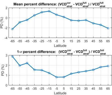
Figure 3. Effect of model scaling of OSIRIS partial VCDs for OSIRIS profiles that terminate ∼3–4 km above the thermal tropopause.(a)Mean and(b)1σ of percent difference of VCDcorstrat minus VCDfullstratwithin 10◦latitude bins.
minate>5 km above the tropopause were excluded from the analysis.
yields profiles that, on average, terminate 3.4 km above the tropopause. VCDcorstrat is then calculated from these profiles using Eq. (3). At most latitudes, VCDcorstrat is within 2 % of VCDfullstrat, which amounts to roughly 5×10¹³molecules cm−2 of the stratospheric VCD, suggesting that the model correc-tions are performing well. This yields conservative estimates because most OSIRIS profiles used in this analysis extend closer to the tropopause, as shown in Fig. 2. However, it should be noted that there is a sampling bias in these tests as OSIRIS profiles that extend below the tropopause are more often available for higher tropopauses.
3.3 Calculation of gridded stratospheric VCD maps
For interpolation to OMI measurements (latitude, longitude, date, local time), daily sets of OSIRIS VCD maps were cre-ated for hourly local times, ranging from 0 to 23 h. Note that the hourly local time resolution of these maps is suffi-cient for interpolation to OMI NO2 measurements because for this study, OMI measurements are used for SZA<75◦ when NO2is not varying rapidly with local time.
In order to calculate these maps, OSIRIS profiles for the time period of interest were selected. Profiles for 65◦S to 65◦N were used to produce VCD maps that were reliable for 60◦S to 60◦N, the latitude range over which OmO is cal-culated. These profiles were scaled to the 0–23 h local time grid using the photochemical box model (see Sect. 3.1) and stratospheric VCDs were calculated from these profiles (see Sect. 3.2).
For each local time, a filtering function was applied to the stratospheric VCDs in order to ensure a smooth field and ac-count for irregular sampling. At each point on the regular grid, a vector of weights is calculated based on the distances between the grid point and the sparse VCD data points (i,j). The weight (wij)for a given sparse VCD data point is then
calculated from the distances between the regular grid point to the sparse point in latitude (1ϕij)and longitude (1λij)
using the following equation:
wij =e
−
1ϕ2 ij 2σϕ2+
1λ2 ij 2σ2 λ
!
, (5)
where σϕ and σλ are standard deviations in the Gaussian
weighting, selected as discussed below. For each regular grid point, if the sum of the weight vector over all sparse VCD data points is <1, the grid point is left empty. Otherwise, the value at the grid point is the mean of the sparse VCDs, weighted by the weighting factors. This essentially smooths the data to a finer grid; a 1◦
latitude and 1◦
longitude grid was used here.
Various combinations of Gaussian weighting standard de-viations and time averaging windows (1-day, 2-day, 3-day, and 5-day) were tested. A 3-day averaging window was se-lected, i.e., each daily map includes measurements from the given date, the previous day, and the next day. Standard de-viations for the Gaussian weighting of 6◦ in latitude and
10◦ longitude were chosen, reflecting the spatial coverage of OSIRIS measurements. These settings yield good spatial coverage in the stratospheric maps, while providing reason-able resolution of features in the VCDs. Due to the averag-ing and smoothaverag-ing of the data, rapid changes or sharp spatial gradients in NO2, for example when vortex remnants reach midlatitudes, may be smoothed out. This is a limitation of OSIRIS sampling.
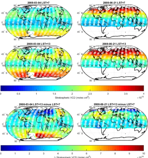
Figure 4 shows examples of the OSIRIS VCD maps for 4 March and 21 June 2008 at the approximate OSIRIS and OMI measurement times. Note that, as described above, each of these maps is made up using 3 days of OSIRIS data. The 4 March VCD maps have global coverage from 65◦S to 65◦N, the latitude range over which OSIRIS profiles were included in the analysis. The 21 June maps have limited coverage in the Southern Hemisphere. This is because OSIRIS does not measure NO2in the winter hemisphere. The VCD maps for 07:00 LT, the approximate OSIRIS measurement time, have lower levels of NO2 than the VCD maps for 13:00 LT, the approximate OMI measurement time. These differences with local time are typically∼0.4–0.5×10¹⁵molecules cm−2and
can locally reach values of up to∼1×10¹⁵molecules cm−2.
This is consistent with the daytime rates of increase in strato-spheric of NO2VCDs measured by Dirksen et al. (2011), us-ing OMI and Système d’Analyse par Observations Zénithal (SAOZ) data. They found increase rates that ranged from ap-proximately 0–4×10¹⁵molecules cm−2h−1, depending on the latitude and time of year, which would correspond to net increases of 0–2.4×10¹⁵molecules cm−2 for the 6 h local time difference in Fig. 4. This demonstrates the effect of the diurnal scaling of NO2 prior to matching the OSIRIS and OMI measurements.
4 Calculation of OMI-minus-OSIRIS (OmO) tropospheric NO2
Figure 4. OSIRIS stratospheric VCD maps for 4 March 2008 (left panels) and 21 June 2008 (right panels). The maps are shown for LST=07:00 (top panels), corresponding to the approximate OSIRIS measurement time, and LST=13:00 (middle panels), corresponding to the approximate OMI measurement time. Difference maps for LST=13:00−07:00 (bottom panels) are also shown. The white circles indicate the locations of the OSIRIS measurements used to create the maps.
4.1 Comparison of stratospheric VCDs from OMI-SP and OSIRIS
In order to obtain an OSIRIS stratospheric VCD for each OMI pixel, a linear interpolation in latitude, longitude, and local time was performed over the OSIRIS stratospheric VCD maps (see Sect. 3.3), corresponding to the OMI surement day. Figure 5 shows the number of OMI-SP mea-surements that were successfully matched to the OSIRIS stratosphere using the OSIRIS gridded VCD maps. In the tropics∼90 % of OMI profiles were matched to the OSIRIS stratosphere. Toward midlatitudes, this drops to∼75–80 %
in the Northern Hemisphere and∼60–70 % in the Southern
Hemisphere, because OSIRIS coverage is limited to the sum-mer hemisphere.
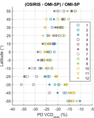
Figure 6 shows a comparison between OMI-SP strato-spheric VCDs and OSIRIS stratostrato-spheric VCDs, interpo-lated from the VCD maps. Percent differences in VCD
were binned according to latitude and month for 2008. The OSIRIS VCDs are smaller than the OMI-SP VCDs for all latitudes and months, with percent differences of∼ −20 to
Figure 5. (a) Number of valid measurements for OMI-SP (blue line) and for OmO (red dashed line). (b) Percent complete-ness of the OmO-SP dataset (number of valid OmO measure-ments/number of valid OMI-SP measurements). Statistics were calculated in 10◦latitude bins.
Figure 6. Mean percent difference of OSIRIS minus OMI-SP stratospheric VCDs (xaxis), binned according to latitude (yaxis) and month (legend). OSIRIS VCDs were interpolated from the OSIRIS gridded VCD maps (see Sect. 3.3) to the OMI measure-ment date, location, and local time. Filtering criteria for the OMI and OSIRIS profiles are given in Sect. 2.1 and 2.2, respectively.
Table 1.Correction factors,γ, applied to the OMI SCDs as a func-tion of the OMI SCD. Correcfunc-tion factors are based on the results of Marchenko et al. (2015) and account for the high bias in the OMI SCDs.
SCD γ
×1016molecules cm−2
0.5755 0.7645
0.8518 0.8049
1.2147 0.8152
1.7336 0.8475
2.3842 0.8721
3.3740 0.8912
4.4346 0.9017
5.4794 0.9082
6.4403 0.9169
7.5376 0.9218
4.2 OMI SCD bias correction
A high bias in the OMI stratospheric VCDs has been ob-served in comparisons with other satellite instruments (Bel-monte Rivas et al., 2014) and is largely explained by a known high bias in the OMNO2A v1 SCDs of roughly 20–30 % due to issues with the spectral fitting (Marchenko et al., 2015; van Geffen et al., 2015). The OMNO2A v1 SCDs are used for both the OMI-DOMINO v2.0 and OMI-SP v2.1 retrievals. OMI tropospheric VCDs are∼10–15 % smaller in polluted regions and ∼30 % smaller in non-polluted regions after SCDs are corrected for the spectral fitting bias (Marchenko et al., 2015).
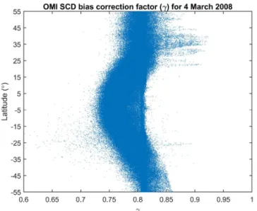
In order to remove systematic mismatches between the OSIRIS stratospheric VCDs and the OMI measurements, the OMI total SCDs were corrected for their high bias. Marchenko et al. (2015) found that the best predictor of the relative SCD bias is the SCD itself, with small SCDs (<5×10¹⁵molecules cm−2)having a∼30 % positive bias and large SCDs (∼5×10¹⁶molecules cm−2)a∼10 % bias. Therefore, the SCD-dependent correction factors shown in Table 1 were applied to the OMI total SCDs, using the methodology described in Sect. 4.3. Outside the range of SCDs listed in Table 1, correction factors were estimated us-ing a linear extrapolation.
Figure 7.OMI SCD bias correction factors versus latitude for OMI-SP measurements on 4 March 2008.
4.3 Calculation of OMI-minus-OSIRIS tropospheric VCD
This section outlines the methodology used to calculate the OmO tropospheric NO2 VCD data product. The OMI total SCD StotOMI
can be expressed as the sum of the stratospheric and tropospheric SCDs SsOMI and StOMI
, which are calcu-lated from the stratospheric and tropospheric AMFs AOMIs
and AOMIt
and VCDs VsOMI andVtOMI
as follows:
StotOMI=SOMIs +StOMI=VsOMI·AOMIs +VtOMI·AOMIt . (6) Similarly, the bias-corrected OMI SCDs can be related to the OSIRIS stratospheric VCD VsOSIRIS
and the inferred (OmO) tropospheric VCD component VtOmO
, using the AMFs from the OMI operational products:
StotOMI·γ =VsOSIRIS·AOMIs +VtOmO·AOMIt , (7) whereγ is the OMI SCD bias correction factor described in Sect. 4.2. Solving for the OmO VCD gives
VtOmO=
γ·StotOMI−VsOSIRIS·AOMIs /AOMIt . (8) An alternate form, and the one used to compute the OmO product, is obtained by combining Eqs. (6) and (8):
VtOmO=γ·VtOMI+
γ·VsOMI−VsOSIRIS
·AOMIs /AOMIt . (9) OmO tropospheric VCDs were computed using AMFs and VCDs from the OMI-SP product. The ratio of AMFs rep-resents the different sensitivities to NO2 located in the troposphere and in the stratosphere. Typically, the ratio
AOMIs /AOMIt is greater than 1, indicating that OMI is more
Figure 8.Annual(a)mean and(b) standard deviation of strato-spheric VCDs for 2008 in 10◦ latitude bins for measurements
with OMI tropospheric VCDs<0.5×10¹⁵molecules cm−2.
Strato-spheric VCDs for OMI-SP (blue circles), OMI-SP scaled byγ(cyan circles), OMI-DOMINO (magenta X’s), OMI-DOMINO scaled by γ(green X’s), and OSIRIS VCD maps interpolated to the OMI mea-surement time/location (red triangles) are shown. Mean and stan-dard deviation are calculated over individual OMI measurements for the entire year.
sensitive to NO2within the stratosphere. OmO was not calcu-lated for the small number of OMI measurements for which the ratio AOMIs /AOMIt >15, indicating that the OMI mea-surement is not very sensitive to the troposphere. For each OMI pixel,VsOSIRISwas interpolated from the OSIRIS grid-ded VCD maps (see Sect. 4.1) andγ was interpolated to the OMI SCD (see Sect. 4.2).
4.4 Matching of OSIRIS and OMI stratospheres
Over unpolluted regions, the OmO tropospheric VCDs should be small and, subsequently, the γ·VsOMI−VsOSIRIS
term in Eq. (9) should also be small. Therefore, the matching of the OSIRIS and OMI stratospheres can be assessed by comparing OSIRIS stratospheric VCDs with OMI VCDs scaled with γ, over unpolluted regions. Figure 8 shows annual average stratospheric VCDs for OMI-SP, OMI-DOMINO, and OSIRIS, binned by lati-tude over unpolluted regions (OMI tropospheric VCDs <
Figure 9.Maps of stratospheric VCDs for 4 March 2008 for OMI-SP (top), OMI-DOMINO (middle), and OSIRIS interpolated to the location of OMI measurements (bottom). Note that different colour scales are used for the OMI and OSIRIS VCDs.
scaled with γ, agreement with OSIRIS is to within 0.2×
1015molecules cm−2 at all latitudes. This suggests that the OMI and OSIRIS stratospheres are well matched. Standard deviations over the year of the individual γ-scaled OMI VCDs are similar to OSIRIS VCDs at most latitudes. At 25, 35◦S, and 55◦N, the standard deviation in the OSIRIS VCDs is larger than the standard deviation in the SP or OMI-DOMINO VCDs.
OMI-SP, OMI-DOMINO, and OSIRIS stratospheric VCD maps are shown for 4 March 2008 in Fig. 9. The OMI VCDs are larger than the OSIRIS VCDs due to the high bias in the OMI SCDs. There is somewhat less structure in the OSIRIS VCDs than in the OMI VCDs. For example, OMI-DOMINO and OMI-SP stratospheric VCDs are enhanced across the northern hemispheric Pacific and Mexico, but enhancements are not as strong in the OSIRIS data. There is a large max-imum in the OMI-DOMINO stratospheric VCDs over east-ern China and Korea, which is not apparent in the OMI-SP or OSIRIS VCDs. These features across the northern
hemi-spheric Pacific and Mexico and over eastern China and Korea all persist in the OMI data over the OSIRIS 3-day sampling period and cover a large enough area that they could be re-solved, although perhaps somewhat distorted, by the OSIRIS VCD maps. Therefore, these local differences between the OSIRIS and OMI stratospheric VCDs cannot be attributed to the smoothing and averaging of the OSIRIS measurements.
4.5 OmO tropospheric VCDs
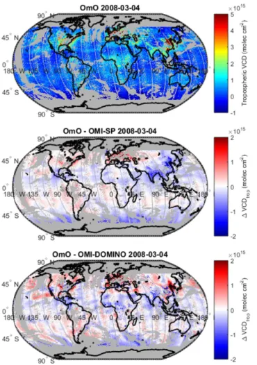
Figure 10 shows the OmO tropospheric VCDs, also for 4 March 2008. At most locations, OmO VCDs are similar to the OMI-SP and OMI-DOMINO VCDs, with a few no-table differences. OmO VCDs are larger than OMI-SP and OMI-DOMINO VCDs over the northern hemispheric Pacific and Mexico, which is consistent with the differences in the observed features in the stratospheric VCDs. OmO VCDs are larger than OMI-DOMINO VCDs over eastern China and Korea, as OmO effectively redistributes NO2from the stratosphere into the troposphere through the second term in Eq. (9). Over much of India and China, OmO VCDs are smaller than the OMI-SP VCDs.
Maps of annual average comparisons between OmO, OMI-SP, and OMI-DOMINO tropospheric NO2are shown in Fig. 11. Over unpolluted regions, differences between OmO and the operational OMI data products are fairly small, sug-gesting that the matching of the OSIRIS and OMI strato-spheres was effective. OmO has less NO2than OMI-SP and OMI-DOMINO over polluted regions such as the eastern United States, Europe, and eastern China. This is expected as the OMI-SP and OMI-DOMINO tropospheric VCDs are bi-ased high by∼10–15 % over polluted regions due to the bias in the SCDs (Marchenko et al., 2015). Over Korea, both the OMI-SP and OmO VCDs are larger than the OMI-DOMINO VCDs. At southern hemispheric midlatitudes, both the OmO and DOMINO VCDs are biased low relative to OMI-SP VCDs. Overall, the differences between the OmO VCDs and the operational OMI data products are within the range of the differences between the two operational OMI data prod-ucts.
Tropospheric VCDs over the Pacific Ocean can be used to assess the quality of the stratosphere–troposphere sepa-ration because tropospheric VCDs are expected to be near background levels. Figure 5 from Hilboll et al. (2013) shows climatological monthly mean tropospheric VCDs over the Pacific (180–150◦W) binned according to month and lati-tude over 1998–2007, as calculated from Oslo CTM2 model simulations (Søvde et al., 2008). At most latitudes, tropo-spheric VCDs are <3×10¹⁴molecules cm−2 according to
the model results. For northern hemispheric midlatitudes, tropospheric VCDs are somewhat larger, ranging from∼2 to
7×10¹⁴molecules cm−2, with the largest values at∼55◦N
in winter months.
Figure 10.Maps of tropospheric VCDs for 4 March 2008 for OmO (top), the difference between OmO and OMI-SP (middle), and the difference between OmO and OMI-DOMINO (bottom).
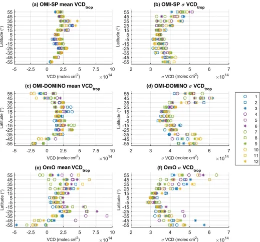
150◦W). The OMI-SP VCDs vary less with latitude and have no mean negative values, unlike the OMI-DOMINO and OmO VCDs. This is expected as the OMI-SP stratosphere– troposphere separation uses measurements over unpolluted regions, including the Pacific, to estimate stratospheric NO2. In the tropics, average VCDs from all three datasets are
<3×10¹⁴molecules cm−2, which is consistent with back-ground levels. At northern hemispheric midlatitudes, OmO mean VCDs increase slightly, ranging from∼2.5×10¹⁴to
∼5×10¹⁴molecules cm−2. This is different from the OMI-SP and OMI-DOMINO VCDs, which mostly remain<3×
1014molecules cm−2, but is consistent with the Oslo CTM2 model simulations. At 55◦
N, both OmO and DOMINO mean VCDs are close to 0 molecules cm−2. In the Southern Hemi-sphere, VCDs for all three datasets decrease with latitude, reaching values near 0 molecules cm−2 in the OMI-SP and negative values in the OMI-DOMINO and OmO datasets at 45 and 55◦S. There are some large outliers in the OmO VCDs for April–July in the Southern Hemisphere, suggest-ing a positive bias in the OmO dataset, likely because the
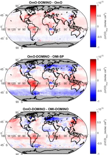
Figure 11.Maps of annual average (top) OmO tropospheric VCDs and differences between tropospheric VCDs for (top-middle) OmO minus OMI-SP, (bottom-middle) OmO minus OMI-DOMINO, and (bottom) OMI-SP minus OMI-DOMINO. Maps are averaged on a 1×1◦grid.
Figure 12.Mean and standard deviation of VCDs in the Pacific (150–180◦W), calculated monthly (legend) in 10◦latitude bins.
(a)
OMI-SP mean VCD,(b)OMI-SP standard deviation of VCD,(c)OMI-DOMINO mean VCD,(d)OMI-DOMINO standard deviation of VCD,
(e)OmO mean VCD, and(f)OmO standard deviation of VCD.
4.6 Alternate OmO-DOMINO tropospheric VCDs
The OmO dataset is affected by the scaling of OSIRIS strato-spheric VCDs to the OMI local times, the OMI SCD bias cor-rection factor, the difference between the OMI and OSIRIS stratospheres, and the choice of the OMI version of AMFs and VCDs (see Eq. 9). In order to gain some insight into the impact of these various terms in the OmO calculation, an alternate OmO-DOMINO dataset was constructed using the OMI-DOMINO VCDs and AMFs (Fig. 13). Over unpol-luted regions, the OmO and OmO-DOMINO VCDs are very similar. Over polluted areas, the OmO-DOMINO VCDs are somewhat larger than the OmO VCDs. However, these dif-ferences are smaller in magnitude than the difdif-ferences be-tween the two OmO products and the operational OMI data products (Figs. 11 and 13). The relative contribution of the various terms in Eq. (9) to the OmO and OmO-DOMINO datasets are discussed in the paragraphs below.
In order to match the OMI and OSIRIS stratospheres, both the OSIRIS and OMI datasets were scaled prior to stratospheric subtraction. The OSIRIS stratospheric VCDs, measured in the morning, were scaled to the OMI af-ternoon local time using a photochemical model,
typi-cally increasing the OSIRIS stratospheric VCDs by∼0.5×
1015molecules cm−2. The OMI SCD bias correction factor was applied to OMI SCDs before creating the OmO and OmO-DOMINO datasets. This correction factor is required in order to properly match the OMI and OSIRIS strato-spheres, for both the OMI-SP and OMI-DOMINO datasets (Fig. 8). Without the correction factor, both the OmO and OmO-DOMINO tropospheric VCDs would be very large (∼
1×10¹⁵molecules cm−2)over the unpolluted Pacific Ocean. After the application of the diurnal variation scaling and OMI SCD bias correction, the OMI-SP, OMI-DOMINO, and OSIRIS stratospheres VCDs agree to within ∼0.2×
Figure 13.Maps of differences between OmO-DOMINO and (top) OmO, (middle) OMI-SP, and (bottom) OMI-DOMINO annual av-erage tropospheric VCDs. Map is avav-eraged on a 1×1◦grid.
The OmO VCDs also depend on the ratio of AMFs (As/At), which scales the difference between the OSIRIS and OMI stratospheric VCDs. Over unpolluted regions, this ratio is∼1.25 and is nearly identical for both OMI-SP and OMI-DOMINO. Over polluted regions, the ratio is larger, reaching annual averages of∼3–4 in some locations. There-fore, differences between OSIRIS and OMI stratospheric VCDs are amplified over polluted areas through the de-pendence on As/At in Eq. (9). Over polluted areas,As/At is somewhat smaller for OMI-SP than for OMI-DOMINO, though the relationship is complicated because Eq. (9) also depends on the OMI tropospheric VCDs, which also differ between the two operational OMI products, primarily over polluted regions (Fig. 11). This is consistent with the ob-served differences between the OmO and OmO-DOMINO datasets, which are largest over polluted areas.
Overall, these tests suggest that the stratospheric matching between OSIRIS and OMI has a larger influence on the OmO dataset than the choice of OMI AMFs. The stratospheric matching currently depends on the OSIRIS and operational OMI stratospheric VCDs, as well as the OMI SCD bias
cor-rection. Considering the complex manner in which biases in SCDs are transferred into the OMI-SP and OMI-DOMINO stratospheric VCD, which can then affect unconstrained (pol-luted) locations, it is impossible at this time to disentangle the impact of the SCD bias from the larger issue of how well each method of stratospheric removal performs. Therefore, the stratospheric matching between OSIRIS and OMI will be better understood once bias-corrected OMI SCDs are avail-able.
5 Summary and future applications
The technique of matching nadir- and limb-viewing satellite retrievals to quantify tropospheric NO2 is explored in this work using OMI nadir measurements and OSIRIS limb mea-surements to create the OmO tropospheric NO2 dataset. As nadir-viewing instruments cannot resolve NO2 in the verti-cal, additional information or assumptions based on unpol-luted regions are required to determine quantities in the up-per and lower atmospheric regions. Currently, there are two operational products for OMI, which estimate stratospheric NO2 using different methods. The OMI-DOMINO product assimilates OMI SCDs into the TM4 model and then sub-tracts modelled stratospheric NO2. The OMI-SP dataset es-timates stratospheric VCDs for locations with background levels of tropospheric NO2 and then uses an extrapolation technique to infer stratospheric VCDs across the globe.
The new OmO tropospheric NO2 dataset uses informa-tion from OSIRIS profile measurements in order to esti-mate the stratospheric contribution to OMI SCD measure-ments. OSIRIS NO2stratospheric VCDs were found to agree to within 0.25×10¹⁵molecules cm−2of the SCIAMACHY, HIRDLS, and MIPAS limb instruments for most latitudes and seasons (Appendix A). OSIRIS profile measurements of stratospheric NO2were scaled to a range of local times us-ing a photochemical model. Stratospheric VCDs were calcu-lated and were gridded onto daily maps of stratospheric NO2 for various local times. The OSIRIS VCD maps were aver-aged over a 3-day window in order to gain sufficient cover-age from the OSIRIS measurements, which could smooth out rapid variations in stratospheric NO2, such as vortex intru-sions. For each OMI measurement, the OSIRIS VCD maps were interpolated to the latitude, longitude, and local time of the OMI measurement. Then the OSIRIS stratospheric VCD and OMI-SP VCDs and AMFs were used to calculate the OmO product for 60◦S–60◦N. In order to match the OSIRIS and OMI data products, corrections for a known bias in OMI SCDs were applied based on the findings of Marchenko et al. (2015). After accounting for a bias in the OMI SCDs, the OSIRIS and OMI annual average stratospheric VCDs agree to within 0.2×10¹⁵molecules cm−2between 60◦S and
The OmO tropospheric VCDs reproduced the broad features of the OMI-SP and OMI-DOMINO tropospheric VCDs. Furthermore, over the Pacific Ocean, the OmO VCDs were consistent with background levels of NO2at most lat-itudes, suggesting that, overall, the stratospheric NO2signal has been successfully removed using the OSIRIS dataset. There are high biases in the OmO dataset for ∼20–40◦S
in April–July, which are consistent with observed system-atic differences between the OSIRIS and OMI stratospheric VCDs for these latitudes and months. Despite this, the matching of the OSIRIS and OMI stratospheres is very good given the rudimentary nature of the OMI SCD-bias cor-rection. No corrections were applied to account for biases between the OSIRIS and OMI datasets. This differs from the technique of Hilboll et al. (2013), who matched SCIA-MACHY limb and nadir measurements through daily cor-rections based on the comparisons over the Pacific Ocean. At present, errors remaining after the simple OMI bias-correction cannot be separated from those in OSIRIS strato-spheric VCD. As such a more quantitative assessment of the potential of this approach can be made only once the next version of OMI SCDs is available.
The results of this study show preliminary success in the compatibility of limb and nadir measurements taken at dif-ferent local times in a simpler framework. This technique could be improved by better accounting for biases between the OMI and OSIRIS datasets. For example, in a full anal-ysis, limb-measured stratospheric NO2and nadir-measured columns could be assimilated together in a chemical trans-port model to estimate stratospheric NO2.
This work underlines the challenge associated with match-ing polar orbitmatch-ing, limb-viewmatch-ing instruments with future geo-stationary nadir-viewing instruments as the measurements occur at many local solar times. By the end of the decade, three instruments, each on board a geostationary satellite will measure NO2in the nadir-viewing geometry: Sentinel-4 (In-gmann et al., 2012) with coverage over Europe, TEMPO (Zoogman et al., 2016) with coverage over North America, and GEMS (Kim, 2012) with coverage over eastern Asia. While this study demonstrates that limb and nadir measure-ments could be matched to retrieve tropospheric NO2, there are currently no planned limb instruments to overlap with these geostationary missions. OSIRIS is well beyond its ex-pected lifetime and there are no planned satellites that can measure stratospheric NO2 beyond 2017, when the Strato-spheric Aerosol and Gas Experiment III (SAGE III) on the International Space Station (ISS) reaches the end of its 1-year design lifetime.
6 Data availability
Figure A1.OSIRIS seasonal mean NO2partial column profiles for
1 February 2005–31 January 2008 in 2◦latitude bins for(a)March–
April–May (MAM),(b)June–July–August (JJA),(c)September–
October–November (SON), and (d) December–January–February
(DJF).
Appendix A: Comparison of OSIRIS NO2to other satellite instruments
In order to assess the OSIRIS v5 NO2product, OSIRIS data for 2005–2007 were compared against the results of Bel-monte Rivas et al. (2014). The study included limb satellite measurements from MIPAS (IMK-IAA version 4.0; Funke et al., 2005), HIRDLS (version 7; Gille et al., 2012), and SCIAMACHY (v3.1; Bauer et al., 2012), as well as satel-lite nadir measurements from OMI (KNMI DOMINO ver-sion 2.0, Boersma et al., 2004, 2011) and SCIAMACHY (KNMI-BIRA TM4NO2A version 2.3; Boersma et al., 2004). Belmonte Rivas et al. (2014) found that the limb stratospheric VCDs from SCIAMACHY-limb, MIPAS, and HIRDLS agree to within 0.25×10¹⁵molecules cm−2, which is better than 10 %, when all observations are adjusted to the HIRDLS local time. Nadir SCIAMACHY and OMI strato-spheric VCDs are biased relative to the limb instruments by−20 % (−0.5×10¹⁵molecules cm−2)and+20 % (0.6×
1015molecules cm−2), respectively.
OSIRIS profiles were averaged using the methodology of Belmonte Rivas et al. (2014). OSIRIS profiles were scaled to the HRDLS local time of∼15:30 LT (Fig. 3 of Belmonte
Rivas et al., 2014), using the photochemical model described in Sect. 2.3 and the methodology described in Sect. 3.1. The photochemical model runs for the 2005–2007 OSIRIS pro-files presented here use the settings described by Brohede et al. (2008). Volume mixing ratio (VMR) profiles were
aver-Figure A2.Seasonal averages of stratospheric NO2VCDs for 1
February 2005–31 January 2008 in 2◦latitude bins for(a)March–
April–May (MAM),(b)June–July–August (JJA),(c)September– October–November (SON), and(d) December–January–February (DJF). SCIAMACHY-limb (blue line), MIPAS (red line), HIRDLS (cyan line), OMI (green dashed line), SCIAMACHY-nadir (grey dashed line), and OSIRIS (thick black line) are all shown. Figure is adapted from Belmonte Rivas et al. (2014).
aged daily in 2◦ latitude bins from 64◦S to 80◦N. Partial column profilesnv(zi)were calculated from the VMRs (V)
using
nv(zi)=10·NA/(g·Mair)·0.5·(Vi+1+Vi)·(pi+1−pi), (A1)
where NA is Avogadro’s constant (6.022×
1023molecules mole−1), g is the Earth’s gravity (9.80 m s−2), and Mair is the molar mass of air (28.97 g mole−1). The pressure increments in hPa were
pi=1000×10−i/24 for i=0–120. Belmonte Rivas et
al. (2014) imposed collocation criteria as well as some smoothing, which were not included here. Therefore, the comparisons presented here are similar to the figures of Belmonte Rivas et al. (2014), but not identical.
measure-ments. This figure is similar to Fig. 8 of Belmonte Ri-vas et al. (2014). OSIRIS stratospheric VCDs are within 0.25×10¹⁵molecules cm−2 of the other limb instruments (SCIAMACHY-limb, MIPAS, and HIRDLS) for most lati-tudes and seasons. However, there are some localised dif-ferences between all four limb instruments of ∼0.5×
Acknowledgements. This work was supported by the Natural Sciences and Engineering Research Council (Canada) and the Canadian Space Agency. Odin is a Swedish-led satellite project funded jointly by Sweden (SNSB), Canada (CSA), France (CNES), and Finland (Tekes). The authors thank David Plummer for the provision of climatological fields from the Canadian Middle Atmosphere Model. Thanks to Sergey Marchenko for providing the OMI SCD bias correction factors. Thank you also to Chris Roth for help with the OSIRIS database.
Edited by: V. Sofieva
Reviewed by: two anonymous referees
References
Bauer, R., Rozanov, A., McLinden, C. A., Gordley, L. L., Lotz, W., Russell III, J. M., Walker, K. A., Zawodny, J. M., Ladstätter-Weißenmayer, A., Bovensmann, H., and Burrows, J. P.: Val-idation of SCIAMACHY limb NO2 profiles using solar
oc-cultation measurements, Atmos. Meas. Tech., 5, 1059–1084, doi:10.5194/amt-5-1059-2012, 2012.
Beirle, S., Kühl, S., Puk¸¯ıte, J., and Wagner, T.: Retrieval of tropo-spheric column densities of NO2from combined SCIAMACHY nadir/limb measurements, Atmos. Meas. Tech., 3, 283–299, doi:10.5194/amt-3-283-2010, 2010.
Belmonte Rivas, M., Veefkind, P., Boersma, F., Levelt, P., Eskes, H., and Gille, J.: Intercomparison of daytime stratospheric NO2
satellite retrievals and model simulations, Atmos. Meas. Tech., 7, 2203–2225, doi:10.5194/amt-7-2203-2014, 2014.
Belmonte Rivas, M., Veefkind, P., Eskes, H., and Levelt, P.: OMI tropospheric NO2profiles from cloud slicing: constraints
on surface emissions, convective transport and lightning NOx,
Atmos. Chem. Phys., 15, 13519–13553, doi:10.5194/acp-15-13519-2015, 2015.
Boersma, K. F., Eskes, H. J., and Brinksma, E. J.: Error analysis for tropospheric NO2retrieval from space, J. Geophys. Res., 109,
D04311, doi:10.1029/2003JD003962, 2004.
Boersma, K. F., Eskes, H. J., Veefkind, J. P., Brinksma, E. J., van der A, R. J., Sneep, M., van den Oord, G. H. J., Levelt, P. F., Stammes, P., Gleason, J. F., and Bucsela, E. J.: Near-real time retrieval of tropospheric NO2from OMI, Atmos. Chem. Phys.,
7, 2103–2118, doi:10.5194/acp-7-2103-2007, 2007.
Boersma, K. F., Eskes, H. J., Dirksen, R. J., van der A, R. J., Veefkind, J. P., Stammes, P., Huijnen, V., Kleipool, Q. L., Sneep, M., Claas, J., Leitão, J., Richter, A., Zhou, Y., and Brunner, D.: An improved tropospheric NO2column retrieval algorithm for the Ozone Monitoring Instrument, Atmos. Meas. Tech., 4, 1905– 1928, doi:10.5194/amt-4-1905-2011, 2011.
Bovensmann, H., Burrows, J. P., Buchwitz, M., Frerick, J., Noël, S., Rozanov, V. V., Chance, K. V., and Goede, A. P. H.: SCIAMACHY: Mission Objectives and Measure-ment Modes, J. Atmos. Sci., 56, 127–150, doi:10.1175/1520-0469(1999)056<0127:SMOAMM>2.0.CO;2, 1999.
Brohede, S., McLinden, C. A., Urban, J., Haley, C. S., Jonsson, A. I., and Murtagh, D.: Odin stratospheric proxy NOy
mea-surements and climatology, Atmos. Chem. Phys., 8, 5731–5754, doi:10.5194/acp-8-5731-2008, 2008.
Brohede, S. M., Haley, C. S., McLinden, C. A., Sioris, C. E., Murtagh, D. P., Petelina, S. V., Llewellyn, E. J., Bazureau, A., Goutail, F., Randall, C. E., Lumpe, J. D., Taha, G., Thomasson, L. W., and Gordley, L. L.: Validation of Odin/OSIRIS strato-spheric NO2 profiles, J. Geophys. Res.-Atmos., 112, D07310,
doi:10.1029/2006JD007586, 2007.
Bucsela, E. J., Celarier, E. A., Wenig, M. O., Gleason, J. F., Veefkind, J. P., Boersma, K. F., and Brinksma, E. J.: Algo-rithm for NO2vertical column retrieval from the ozone monitor-ing instrument, IEEE T. Geosci. Remote Sens., 44, 1245–1258, doi:10.1109/TGRS.2005.863715, 2006.
Bucsela, E. J., Krotkov, N. A., Celarier, E. A., Lamsal, L. N., Swartz, W. H., Bhartia, P. K., Boersma, K. F., Veefkind, J. P., Gleason, J. F., and Pickering, K. E.: A new stratospheric and tropospheric NO2retrieval algorithm for nadir-viewing satellite
instruments: applications to OMI, Atmos. Meas. Tech., 6, 2607– 2626, doi:10.5194/amt-6-2607-2013, 2013.
Burrows, J. P., Weber, M., Buchwitz, M., Rozanov, V.,
Ladstätter-Weißenmayer, A., Richter, A., DeBeek, R.,
Hoogen, R., Bramstedt, K., Eichmann, K.-U., Eisinger, M., and Perner, D.: The Global Ozone Monitoring Experiment (GOME): Mission, instrument concept, and first scientific results, J. Atmos. Sci., 56, 151–175, doi:10.1175/1520-0469(1999)056<0151:TGOMEG>2.0.CO;2, 1999.
Callies, J., Corpaccioli, E., Eisinger, M., Hahne, A., and Lefebvre, A.: GOME-2 – Metop’s second-generation sensor for operational ozone monitoring, ESA Bull. Sp. Agency, 102, 28–36, 2000. Chance, K. V. and Spurr, R. D.: Ring effect studies: Rayleigh
scattering, including molecular parameters for rotational Raman scattering, and the Fraunhofer spectrum, Appl. Opt., 36, 5224– 5230, doi:10.1364/AO.36.005224, 1997.
Choi, S., Joiner, J., Choi, Y., Duncan, B. N., Vasilkov, A., Krotkov, N., and Bucsela, E.: First estimates of global free-tropospheric NO2 abundances derived using a cloud-slicing technique ap-plied to satellite observations from the Aura Ozone Monitor-ing Instrument (OMI), Atmos. Chem. Phys., 14, 10565–10588, doi:10.5194/acp-14-10565-2014, 2014.
Degenstein, D. A., Bourassa, A. E., Roth, C. Z., and Llewellyn, E. J.: Limb scatter ozone retrieval from 10 to 60 km using a multiplicative algebraic reconstruction technique, Atmos. Chem. Phys., 9, 6521–6529, doi:10.5194/acp-9-6521-2009, 2009. Dirksen, R. J., Boersma, K. F., Eskes, H. J., Ionov, D. V., Bucsela,
E. J., Levelt, P. F., and Kelder, H. M.: Evaluation of stratospheric NO2retrieved from the Ozone Monitoring Instrument:
Intercom-parison, diurnal cycle, and trending, J. Geophys. Res.-Atmos., 116, D08305, doi:10.1029/2010JD014943, 2011.
Duncan, B. N., Lamsal, L. N., Thompson, A. M., Yoshida, Y., Lu, Z., Streets, D. G., Hurwitz, M. M., and Pickering, K. E.: A space-based, high-resolution view of notable changes in urban NO2
pollution around the world (2004–2014), J. Geophys. Res., 121, 976–996, doi:10.1002/2015JD024121, 2016.
Funke, B., López-Puertas, M., von Clarmann, T., Stiller, G. P., Fischer, H., Glatthor, N., Grabowski, U., Höpfner, M., Kell-mann, S., Kiefer, M., Linden, A., Mengistu Tsidu, G., Milz, M., Steck, T., and Wang, D. Y.: Retrieval of stratospheric NOxfrom
5.3 and 6.2 µm nonlocal thermodynamic equilibrium emissions measured by Michelson Interferometer for Passive Atmospheric Sounding (MIPAS) on Envisat, J. Geophys. Res., 110, D09302, doi:10.1029/2004JD005225, 2005.
Gille, J., Barnett, J., Arter, P., Barker, M., Bernath, P., Boone, C., Cavanaugh, C., Chow, J., Coffey, M., Craft, J., Craig, C., Di-als, M., Dean, V., Eden, T., Edwards, D. P., Francis, G., Halvor-son, C., Harvey, L., Hepplewhite, C., Khosravi, R., KinniHalvor-son, D., Krinsky, C., Lambert, A., Lee, H., Lyjak, L., Loh, J., Mankin, W., Massie, S., McInerney, J., Moorhouse, J., Nardi, B., Pack-man, D., Randall, C., Reburn, J., Rudolf, W., Schwartz, M., Ser-afin, J., Stone, K., Torpy, B., Walker, K., Waterfall, A., Watkins, R., Whitney, J., Woodard, D., and Young, G.: High Resolution Dynamics Limb Sounder: Experiment overview, recovery, and validation of initial temperature data, J. Geophys. Res.-Atmos., 113, D16S43, doi:10.1029/2007JD008824, 2008.
Gille, J., Cavanaugh, C., Halvorson, C., Hartsough, C., Nardi, B., Rivas, M., Khosravi, R., Smith, L., and Francis, G.: Final correc-tion algorithms for HIRDLS version 7 data, Proc. SPIE, 8511, 85110K, doi:10.1117/12.930175, 2012.
Haley, C. S. and Brohede, S.: Status of the Odin/OSIRIS strato-spheric O3and NO2data products, Can. J. Phys., 85, 1177–1194,
doi:10.1139/P07-114, 2007.
Hendrick, F., Van Roozendael, M., Kylling, A., Petritoli, A., Rozanov, A., Sanghavi, S., Schofield, R., von Friedeburg, C., Wagner, T., Wittrock, F., Fonteyn, D., and De Mazière, M.: In-tercomparison exercise between different radiative transfer mod-els used for the interpretation of ground-based zenith-sky and multi-axis DOAS observations, Atmos. Chem. Phys., 6, 93–108, doi:10.5194/acp-6-93-2006, 2006.
Hilboll, A., Richter, A., Rozanov, A., Hodnebrog, Ø., Heckel, A., Solberg, S., Stordal, F., and Burrows, J. P.: Improvements to the retrieval of tropospheric NO2from satellite – stratospheric
cor-rection using SCIAMACHY limb/nadir matching and compari-son to Oslo CTM2 simulations, Atmos. Meas. Tech., 6, 565–584, doi:10.5194/amt-6-565-2013, 2013.
Ingmann, P., Veihelmann, B., Langen, J., Lamarre, D., Stark, H., and Courrèges-Lacoste, G. B.: Requirements for the GMES Atmosphere Service and ESA’s implementation con-cept: Sentinels-4/-5 and -5p, Remote Sens. Environ., 120, 58–69, doi:10.1016/j.rse.2012.01.023, 2012.
Jonsson, A. I., de Grandpré, J., Fomichev, V. I., McConnell, J. C., and Beagley, S. R.: Doubled CO2-induced cooling
in the middle atmosphere: Photochemical analysis of the ozone radiative feedback, J. Geophys. Res., 109, D24103, doi:10.1029/2004JD005093, 2004.
Kalnay, E., Kanamisu, M., Kistler, R., Collins, W., Deaven, D., Gandin, L., Iredell, M., Saha, S., White, G., Woollen, J., Zhu, Y., Chelliah, M., Ebisuzaki, W., Higgins, W., Janowiak, J., Mo, K. C., Ropelewski, C., Wang, J., Leetmaa, A., Reynolds, R., Jenne, R., and Dennis, J.: The NCEP/NCAR 40 Year Reanalysis Project, B. Am. Meteorol. Soc., 77, 437–471, doi:10.1175/1520-0477(1996)077<0437:TNYRP>2.0.CO;2, 1996.
Kerzenmacher, T., Wolff, M. A., Strong, K., Dupuy, E., Walker, K. A., Amekudzi, L. K., Batchelor, R. L., Bernath, P. F., Berthet,
G., Blumenstock, T., Boone, C. D., Bramstedt, K., Brogniez, C., Brohede, S., Burrows, J. P., Catoire, V., Dodion, J., Drummond, J. R., Dufour, D. G., Funke, B., Fussen, D., Goutail, F., Grif-fith, D. W. T., Haley, C. S., Hendrick, F., Höpfner, M., Huret, N., Jones, N., Kar, J., Kramer, I., Llewellyn, E. J., López-Puertas, M., Manney, G., McElroy, C. T., McLinden, C. A., Melo, S., Mikuteit, S., Murtagh, D., Nichitiu, F., Notholt, J., Nowlan, C., Piccolo, C., Pommereau, J.-P., Randall, C., Raspollini, P., Ri-dolfi, M., Richter, A., Schneider, M., Schrems, O., Silicani, M., Stiller, G. P., Taylor, J., Tétard, C., Toohey, M., Vanhellemont, F., Warneke, T., Zawodny, J. M., and Zou, J.: Validation of NO2and
NO from the Atmospheric Chemistry Experiment (ACE), At-mos. Chem. Phys., 8, 5801–5841, doi:10.5194/acp-8-5801-2008, 2008.
Kim, J.: GEMS (Geostationary Environment Monitoring Spectrom-eter) onboard the GeoKOMPSAT to Monitor Air Quality in high Temporal and Spatial Resolution over Asia-Pacific Region, EGU General Assembly 2012, Vienna, Austria, 22–27 April 2012, 4051, 2012.
Krotkov, N. A., McLinden, C. A., Li, C., Lamsal, L. N., Celarier, E. A., Marchenko, S. V., Swartz, W. H., Bucsela, E. J., Joiner, J., Duncan, B. N., Boersma, K. F., Veefkind, J. P., Levelt, P. F., Fioletov, V. E., Dickerson, R. R., He, H., Lu, Z., and Streets, D. G.: Aura OMI observations of regional SO2and NO2
pollu-tion changes from 2005 to 2015, Atmos. Chem. Phys., 16, 4605– 4629, doi:10.5194/acp-16-4605-2016, 2016.
Lamsal, L. N., Krotkov, N. A., Celarier, E. A., Swartz, W. H., Pick-ering, K. E., Bucsela, E. J., Gleason, J. F., Martin, R. V., Philip, S., Irie, H., Cede, A., Herman, J., Weinheimer, A., Szykman, J. J., and Knepp, T. N.: Evaluation of OMI operational standard NO2
column retrievals using in situ and surface-based NO2
observa-tions, Atmos. Chem. Phys., 14, 11587–11609, doi:10.5194/acp-14-11587-2014, 2014.
Levelt, P. F., Van den Oord, G. H. J., Dobber, M. R., Mälkki, A., Visser, H., de Vries, J., Stammes, P., Lundell, J. O. V., and Saari, H.: The ozone monitoring instrument, IEEE T. Geosci. Remote Sens., 44, 1093–1101, doi:10.1109/TGRS.2006.872333, 2006. Llewellyn, E. J., Lloyd, N. D., Degenstein, D. A., Gattinger, R. L.,
Petelina, S. V., Bourassa, A. E., Wiensz, J. . T., Ivanov, E. V., McDade, I. C., Solheim, B. H., McConnell, J. C., Haley, C. S., von Savigny, C., Sioris, C. E., McLinden, C. A., Griffioen, E., Kaminski, J., Evans, W. F. J., Puckrin, E., Strong, K., Wehrle, V., Hum, R. H., Kendall, D. J. W., Matsushita, J., Murtagh, D. P., Brohede, S., Stegman, J., Witt, G., Barnes, G., Payne, W. F., Piché, L., Smith, K., Warshaw, G., Deslauniers, D.-L., Marc-hand, P., Richardson, E. H., King, R. A., Wevers, I., McCreath, W., Kyrölä, E., Oikarinen, L., Leppelmeier, G. W., Auvinen, H., Mégie, G., Hauchecorne, A., Lefèvre, F., de La Nöe, J., Ricaud, P., Frisk, U., Sjoberg, F., von Schéele, F., and Nordh, L.: The OSIRIS instrument on the Odin spacecraft, Can. J. Phys., 82, 411–422, doi:10.1139/p04-005, 2004.
Marchenko, S., Krotkov, N. A., Lamsal, L. N., Celarier, E. A., Swartz, W. H., and Bucsela, E. J.: Revising the slant column den-sity retrieval of nitrogen dioxide observed by the Ozone Mon-itoring Instrument, J. Geophys. Res.-Atmos., 120, 5670–5692 , doi:10.1002/2014JD022913, 2015.
im-proved retrieval of tropospheric nitrogen dioxide from GOME, J. Geophys. Res.-Atmos., 107, 4437, doi:10.1029/2001JD001027, 2002.
McLinden, C. A., Olsen, S. C., Hannegan, B., Wild, O., Prather, M. J., and Sundet, J.: Stratospheric ozone in 3-D models: A simple chemistry and the cross-tropopause flux, J. Geophys. Res., 105, 14653–14665, doi:10.1029/2000JD900124, 2000.
McLinden, C. A., Haley, C. S., and Sioris, C. E.: Diurnal ef-fects in limb scatter observations, J. Geophys. Res.-Atmos., 111, D14302, doi:10.1029/2005JD006628, 2006.
McLinden, C. A., Fioletov, V., Boersma, K. F., Krotkov, N., Sioris, C. E., Veefkind, J. P., and Yang, K.: Air quality over the Cana-dian oil sands: A first assessment using satellite observations, Geophys. Res. Lett., 39, L04804, doi:10.1029/2011GL050273, 2012a.
McLinden, C. A., Bourassa, A. E., Brohede, S., Cooper, M., De-genstein, D. A., Evans, W. J. F., Gattinger, R. L., Haley, C. S., Llewellyn, E. J., Lloyd, N. D., Loewen, P., Martin, R. V., Mc-Connell, J. C., McDade, I. C., Murtagh, D., Rieger, L., Von Sav-igny, C., Sheese, P. E., Sioris, C. E., Solheim, B., and Strong, K.: Osiris: A Decade of scattered light, B. Am. Meteorol. Soc., 93, 1845–1863, doi:10.1175/BAMS-D-11-00135.1, 2012b. Murtagh, D., Frisk, U., Merino, F., Ridal, M., Jonsson, A., Stegman,
J., Witt, G., Eriksson, P., Jiménez, C., Megie, G., Noë, J. D. La, Ricaud, P., Baron, P., Pardo, J. R., Hauchcorne, A., Llewellyn, E. J., Degenstein, D. A., Gattinger, R. L., Lloyd, N. D., Evans, W. F. J., McDade, I. C., Haley, C. S., Sioris, C., von Savigny, C., Solheim, B. H., McConnell, J. C., Strong, K., Richardson, E. H., Leppelmeier, G. W., Kyrölä, E., Auvinen, H., and Oikarinen, L.: An overview of the Odin atmospheric mission, Can. J. Phys., 80, 309–319, doi:10.1139/p01-157, 2002.
Prather, M.: Catastrophic loss of stratospheric ozone in dense
volcanic clouds, J. Geophys. Res., 97, 10187–10191,
doi:10.1029/92JD00845, 1992.
Richter, A. and Burrows, J. P.: Tropospheric NO2from GOME
mea-surements, Adv. Space Res., 29, 1673–1683, doi:10.1016/S0273-1177(02)00100-X, 2002.
Richter, A., Burrows, J. P., Nüß, H., Granier, C., and Niemeier, U.: Increase in tropospheric nitrogen dioxide over China observed from space, Nature, 437, 129–132, doi:10.1038/nature04092, 2005.
Rieger, L. A., Bourassa, A. E., and Degenstein, D. A.: Merging the OSIRIS and SAGE II stratospheric aerosol records, J. Geophys. Res., 12, 1–15, doi:10.1002/2015JD023133, 2015.
Russell, A. R., Valin, L. C., and Cohen, R. C.: Trends in OMI NO2
observations over the United States: effects of emission control technology and the economic recession, Atmos. Chem. Phys., 12, 12197–12209, doi:10.5194/acp-12-12197-2012, 2012.
Schoeberl, M. R., Douglass, A. R., Hilsenrath, E., Bhartia, P. K., Beer, R., Waters, J. W., Gunson, M. R., Froidevaux, L., Gille, J. C., Barnett, J. J., Levelt, P. F., and DeCola, P.: Overview of the EOS aura mission, IEEE T. Geosci. Remote Sens., 44, 1066– 1072, doi:10.1109/TGRS.2005.861950, 2006.
Scinocca, J. F., McFarlane, N. A., Lazare, M., Li, J., and Plummer, D.: Technical Note: The CCCma third generation AGCM and its extension into the middle atmosphere, Atmos. Chem. Phys., 8, 7055–7074, doi:10.5194/acp-8-7055-2008, 2008.
Sierk, B., Richter, A., Rozanov, A., Von Savigny, C., Schmoltner, A. M., Buchwitz, M., Bovensmann, H., and Burrows, J. P.: Retrieval and monitoring of atmospheric trace gas concentrations in nadir and limb geometry using the space-borne SCIAMACHY instru-ment, Environ. Monit. Assess., 120, 65–77, doi:10.1007/s10661-005-9049-9, 2006.
Sioris, C. E., Kurosu, T. P., Martin, R. V., and Chance, K.: Stratospheric and tropospheric NO2 observed by
SCIA-MACHY: First results, Adv. Space Res., 34, 780–785, doi:10.1016/j.asr.2003.08.066, 2004.
Søvde, O. A., Gauss, M., Smyshlyaev, S. P., and Isaksen, I. S. A.: Evaluation of the chemical transport model Oslo CTM2 with focus on arctic winter ozone depletion, J. Geophys. Res., 113, D09304, doi:10.1029/2007JD009240, 2008.
van Geffen, J. H. G. M., Boersma, K. F., Van Roozendael, M., Hen-drick, F., Mahieu, E., De Smedt, I., Sneep, M., and Veefkind, J. P.: Improved spectral fitting of nitrogen dioxide from OMI in the 405–465 nm window, Atmos. Meas. Tech., 8, 1685–1699, doi:10.5194/amt-8-1685-2015, 2015.
Veefkind, J. P., Boersma, K. F., Wang, J., Kurosu, T. P., Krotkov, N., Chance, K., and Levelt, P. F.: Global satellite analysis of the rela-tion between aerosols and short-lived trace gases, Atmos. Chem. Phys., 11, 1255–1267, doi:10.5194/acp-11-1255-2011, 2011. Zhou, Y., Brunner, D., Hueglin, C., Henne, S. and
Stae-helin, J.: Changes in OMI tropospheric NO2 columns
over Europe from 2004 to 2009 and the influence of meteorological variability, Atmos. Environ., 46, 482–495, doi:10.1016/j.atmosenv.2011.09.024, 2012.