Deriving a sea surface climatology of CO<sub>2</sub> fugacity in support of air–sea gas flux studies

(1)

OSD

11, 1895–1948, 2014

Deriving a sea surface CO2

climatology

L. M. Goddijn-Murphy et al.

Title Page

Abstract Introduction

Conclusions References

Tables Figures

◭ ◮

Back Close

Full Screen / Esc

Printer-friendly Version

Interactive Discussion

Discussion

P

a

per

|

Discus

sion

P

a

per

|

Discussion

P

a

per

|

Discussion

P

a

per

|

Ocean Sci. Discuss., 11, 1895–1948, 2014 www.ocean-sci-discuss.net/11/1895/2014/ doi:10.5194/osd-11-1895-2014

This discussion paper is/has been under review for the journal Ocean Science (OS). Please refer to the corresponding final paper in OS if available.

Deriving a sea surface climatology of CO

₂

fugacity in support of air–sea gas flux

studies

L. M. Goddijn-Murphy1, D. K. Woolf2, P. E. Land3, J. D. Shutler3, and C. Donlon4

1

ERI, University of the Highlands and Islands, Ormlie Road, Thurso, UK 2

ICIT, Heriot-Watt University, Stromness, UK 3

Plymouth Marine Laboratory, Prospect Place, Plymouth, UK 4

European Space Agency/ESTEC, Noordwijk, the Netherlands

Received: 27 June 2014 – Accepted: 8 July 2014 – Published: 28 July 2014

Correspondence to: L. M. Goddijn-Murphy (lonneke.goddijn-murphy@uhi.ac.uk)

Published by Copernicus Publications on behalf of the European Geosciences Union.

(2)

OSD

11, 1895–1948, 2014

climatology

Title Page

Tables Figures

◭ ◮

Back Close

Full Screen / Esc

Discussion

P

a

per

|

Discus

sion

P

a

per

|

Discussion

P

a

per

|

Discussion

P

a

per

|

Abstract

Climatologies, or long-term averages, of essential climate variables are useful for eval-uating models and providing a baseline for studying anomalies. The Surface Ocean Carbon Dioxide (CO₂) Atlas (SOCAT) has made millions of global underway sea sur-face measurements of CO2publicly available, all in a uniform format and presented as

5

fugacity,fCO₂.fCO₂ is highly sensitive to temperature and the measurements are only

valid for the instantaneous sea surface temperature (SST) that is measured concurrent with the in-water CO2 measurement. To create a climatology of fCO₂ data suitable for

calculating air–sea CO2 fluxes it is therefore desirable to calculate fCO₂ valid for

cli-mate quality SST. This paper presents a method for creating such a climatology. We

10

recomputed SOCAT’s fCO₂ values for their respective measurement month and year

using climate quality SST data from satellite Earth observation and then extrapolated the resultingfCO₂ values to reference year 2010. The data were then spatially

interpo-lated onto a 1◦_×1◦ grid of the global oceans to produce 12 monthlyfCO₂ distributions

for 2010. The partial pressure of CO₂ (pCO₂) is also provided for those who prefer to

15

use pCO₂. The CO2 concentration difference between ocean and atmosphere is the

thermodynamic driving force of the air–sea CO2 flux, and hence the presented fCO₂

distributions can be used in air–sea gas flux calculations together with climatologies of other climate variables.

1 Background

20

1.1 Introduction

Observations demonstrate that dissolved CO2 concentrations in the surface ocean

have been increasing nearly everywhere, roughly following the atmospheric CO₂ in-crease but with large regional and temporal variability (Takahashi et al., 2009; McKinley et al., 2011). In general, tropical waters release CO2 to the atmosphere, whereas

(3)

OSD

11, 1895–1948, 2014

climatology

Title Page

Tables Figures

◭ ◮

Back Close

Full Screen / Esc

Discussion

P

a

per

|

Discus

sion

P

a

per

|

Discussion

P

a

per

|

Discussion

P

a

per

|

high-latitude oceans take up CO₂from the atmosphere. Accurate knowledge of air–sea fluxes of heat, gas and momentum is essential for assessing the ocean’s role in climate variability, understanding climate dynamics, and forcing ocean/atmosphere models for predictions from days to centuries (Wanninkhof et al., 2009).

The European Space Agency OceanFlux Greenhouse Gases (GHG) project (http:

5

//www.oceanflux-ghg.org/) is an initiative to improve the quantification of air–sea ex-changes of greenhouse gases such as CO₂. The project has developed datasets suit-able for computation of gas flux climatology in which mean gridded values are com-puted from multiple measurements over different years. The gas flux calculation re-quires accurate values of gas transfer velocity, in addition to the concentrations of the

10

dissolved gas above and below the air-water interface (Liss and Merlivat, 1986). The project has relied heavily on the data sets successfully developed and maintained by the Surface Ocean CO2Atlas (SOCAT, Bakker et al., 2013; Pfeil et al., 2013; Sabine

et al., 2013). SOCAT has collated and carefully quality-controlled the largest collection of ocean CO2observations providing data in an agreed and controlled format for

scien-15

tific activities. Recognising that some groups may have trouble working with millions of measurements, the SOCAT gridded product (Sabine et al., 2013) was then generated to provide a robust, regularly spaced fCO₂ product with minimal spatial and temporal

interpolation. This gridded climatology is useful for evaluating models and for studying and characterisingfCO₂ variations within regions in a format that is easy to exploit.

20

Gas concentrations of CO2 in the upper ocean can be derived from SOCAT’s

un-derway sea surface measurements of fugacity,fCO₂ (pCO₂ adjusted to account for the

fact that the gas is not ideal regarding molecular interactions between the gas and the air). The aquatic CO2 concentration can be expressed as the product offCO₂ and

sol-ubility of CO2and the product of CO2concentration and gas transfer velocity,k, gives

25

us the air–sea gas flux. Di_fferent Authors of CO₂ ocean-atmosphere gas flux prod-ucts use either a mean value offCO₂ (e.g. Sabine et al., 2013) orpCO₂ (e.g. Takahashi

2002, 2009) within a grid box for a particular measurement month and year. Many studies have used thepCO₂ climatology of Takahashi et al. (2002, 2009) as a basis to

(4)

OSD

11, 1895–1948, 2014

climatology

Title Page

Tables Figures

◭ ◮

Back Close

Full Screen / Esc

Discussion

P

a

per

|

Discus

sion

P

a

per

|

Discussion

P

a

per

|

Discussion

P

a

per

|

estimate their own air–sea fluxes (e.g., Kettle et al., 2005, 2009; Fangohr and Woolf 2007; Land et al., 2013). The datasets from Takahashi et al. (2002, 2009) and Sabine et al. (2013) are calculated using in situ SST obtained at depth (SSTdepth) for the

con-struction of ocean CO₂ flux climatology (in situfCO₂ is derived fromfCO₂ measured in

the shipboard equilibrator using the difference between the temperature of sea water

5

in the equilibrator and SSTdepth). BecausefCO₂ is highly sensitive to temperature

fluc-tuations, an instantaneous measurement off_CO

2 is only really valid for its concurrent in

situ SSTdepth measurement. Takahashi et al. (2009) explain that under-sampling and

their interpolation method lead to differences between their pCO₂ values with the true

climatological mean values. They estimate a mean +0.08◦C temperature difference,

10

introducing a systematic bias of about+1.3 µatm in the mean surface waterpCO₂ over

all monthly mean values obtained in their study. Takahashi et al. (2009) also acknowl-edge that by using SSTdepth in their calculations, surface-layer effects could introduce

systematic errors in the sea-airpCO₂ differences but leave that for future research.

Ad-ditional SST biases are introduced by different measurement systems that measure

15

SST at sea and that are each associated with typical measurement biases. All biases in SST, and hence infCO₂, contribute to uncertainties in the true monthly means offCO₂.

A true monthly mean value offCO₂ should therefore be estimated by calculating fCO₂

for a monthly mean value of SST; using these values a climatology offCO₂ applicable

to air–sea gas flux climatology can then be derived.

20

The focus of this paper is to critically assessfCO₂ calculations and the application of

fCO₂ for CO2 ocean gas flux climatology development, in particular the need to

prop-erly address the implications of using different SST. We first review the importance of SST on the calculation off_CO

2 and the use of satellite SST data. We then review the

monthly composite SST data provided by SOCAT and compare those to satellite

ob-25

servations of SST. In Sect. 2 we describe the SOCAT data set and methods, followed by an explanation of our alternative approach to computation of in situf_CO

2 to

clima-tologicalfCO₂ (Sect. 3). In Sect. 4 the spatial interpolation using ordinary block kriging

(5)

OSD

11, 1895–1948, 2014

climatology

Title Page

Tables Figures

◭ ◮

Back Close

Full Screen / Esc

Discussion

P

a

per

|

Discus

sion

P

a

per

|

Discussion

P

a

per

|

Discussion

P

a

per

|

are discussed. Our application of the recently released SOCAT version 2 data set is the subject of Sect. 6. In the conclusion (Sect. 7) the different data products and their uses are compared. The month January is used as an illustrative example of the data treatment throughout this paper.

1.2 Complexities of in situ SST measurements and implications forfCO2

5

As already discussed,fCO₂ is highly sensitive to temperature. Similarly accurate

knowl-edge of SST and, to a lesser extent, salinity, is essential when calculating air–sea gas fluxes. SST vertical profiles are complex and variable. SST can also vary over rela-tively short time scales within relarela-tively small regions and variations in the temperature measured can also arise from the method and instrumentation used for measuring it.

10

All of these issues can cause problems when using in situ data to construct an fCO₂

climatology. These issues are now discussed.

The structure of the upper ocean (_∼10 m) vertical temperature profile depends on the level of shear driven ocean turbulence and the air–sea fluxes of heat, moisture and momentum. Thus, every SST observation depends on the measurement technique

15

and sensor that is used, the vertical position of the measurement within the water col-umn, the local history of all components of the heat flux conditions and, the time of day the measurement was obtained (Donlon et al., 2002). The subsurface SST, SST_depth (see Donlon et al., 2007) will encompass any temperature within the water column where turbulent heat transfer processes dominate. Such a measurement may be

sig-20

nificantly influenced by local solar heating, the variations of which have a time scale of hours and typically varies with depth. This diurnal warming occurs at the sea sur-face when incoming shortwave radiation leads to stratification of the sursur-face water in the absence of wind-induced mixing and temperature di_fferences of >3 K can occur across the surface warm layer (Ward et al., 2004), which in turn will enhance the

out-25

gassing flux of CO2 (Jeffery et al., 2007, 2008; Kettle et al., 2009) that reduces the

oceanic carbon uptake (Olsen et al., 2004). Consequently to help address this sort of issue the international Group on High Resolution Sea Surface Temperature (GHRSST)

(6)

OSD

11, 1895–1948, 2014

climatology

Title Page

Tables Figures

◭ ◮

Back Close

Full Screen / Esc

Discussion

P

a

per

|

Discus

sion

P

a

per

|

Discussion

P

a

per

|

Discussion

P

a

per

|

state that SST_depth should always be quoted at a specific depth in the water column; e.g., SST5 mrefers to the SST at a depth of 5 m. However, SSTdepth data can be

mea-sured using a variety of different temperature sensors mounted on buoys, profilers and ships at any depth beneath the water skin and the depth of the measurement is often not recorded. Different measurement systems that are used to measure SST (e.g. hull

5

mounted thermistors, inboard thermosalinograph systems) have evolved over time us-ing different techniques that are prone to different error characteristics (e.g. for a good review see Kennedy, 2013; Kennedy et al., 2011a, b), such as warming of water as it passes through the ships’ internal pipes before reaching an inboard thermosalinograph (e.g. Kent et al., 1993; Emery et al., 2001; Reynolds et al., 2010; Kennedy, 2013), poor

10

calibration or biases due to the location and warming of hull mounted temperature sensors (e.g. Emery et al., 1997, 2001), inadequate knowledge of temperature sensor depth (e.g. Emery et al., 1997; Donlon et al., 2007), poor knowledge of temperature sensor calibration performance and local thermal stratification during a diurnal cycle (e.g., Kawai and Wada, 2007). This means that if not carefully controlled, SST biases

15

of>1 K may easily be introduced into an in situ SST dataset.

All of these issues mean that directly using SST andfCO₂ measurement pairs from

a large dataset (i.e., that resulting from a large number of different instrument setups and methods) to afCO₂ climatology for studying air–sea gas fluxes is likely to introduce

a source of error. Therefore, we propose that correcting all of the fCO₂ data back to

20

a consistent surface SST dataset is clearly advantageous and this is where satellite data can provide help.

1.3 The use of satellite sea surface temperature data

Satellite Earth observation thermal infrared radiometers used to sense sea skin tem-perature variations have been in orbit around the Earth since the 1990s. The resultant

25

(7)

OSD

11, 1895–1948, 2014

climatology

Title Page

Tables Figures

◭ ◮

Back Close

Full Screen / Esc

Discussion

P

a

per

|

Discus

sion

P

a

per

|

Discussion

P

a

per

|

Discussion

P

a

per

|

(Merchant et al., 2008, 2012). We used ARC SST values from the Along Track Scan-ning Radiometers, ATSRs, Reprocessing for Climate project, ARC, (Merchant et al., 2012). This climate data record is a global, long-term, homogenous, highly stable SST dataset based on satellite derived SST observations.

The difference in the fugacities of CO2 across the diffusive sub-layer at the ocean

5

surface is the driving force behind the air–sea flux of CO2. As discussed above in situ

sub-surface seawater fugacity is normally measured several meters below the surface. Implied in the use of these measurements for deriving air–sea fluxes is the assumption that the measured fugacity values at depth are the same as those at the bottom of the diffusive boundary layer. Diurnal stratification of the surface ocean further complicates

10

this situation. At wind speeds of approximately 6 m s−1 and above, the relationship between the SST (at the sea skin) and SST (at depth and below the diffusive sub layer), is well characterized for both day- and night-time conditions by a cool bias (e.g. Donlon et al., 2002). Therefore a skin temperature value from EO with an appropriate correction for the cool skin bias can be used to describe the temperature below the

15

diffusive sub layer. This means that this temperature value can be used to correct the

fCO₂ from depth to the value below the diffusive sub layer.

1.4 A comparison between SST datasets

In air–sea gas flux calculations an estimate of the water side fCO₂, and hence the

temperature, is required at the base of the mass boundary layer. However, ARC

20

SST is measured at the sea surface skin, SST_skin, which is characteristically cooler than the water just below it during the night but subject to local diurnal variabil-ity and thermal stratification during the day. We derived subskin SST (the SST at the base of the thermal boundary layer) from ARC SST by accounting for the “cool skin effect”. Since gas transfer velocities are low in low wind speeds, it is more

im-25

portant to have a reasonably accurate estimate of the thermal skin effect in mod-erate and high wind speeds. Donlon et al. (1999) reported a mean cool skin _∆T =

(8)

OSD

11, 1895–1948, 2014

climatology

Title Page

Tables Figures

◭ ◮

Back Close

Full Screen / Esc

Discussion

P

a

per

|

Discus

sion

P

a

per

|

Discussion

P

a

per

|

Discussion

P

a

per

|

approximation of the water temperature in the meters below the surface, SST_depth (Donlon et al., 1999; 2002). According to Kettle et al. (2009) the difference between

fCO₂ for the temperature at the base of the mass boundary layer, andfCO₂ for SSTdepth

is negligible so we calculated fCO₂ using subskin SST to estimate fCO₂ at the base

of the mass boundary layer. The ARC dataset provides SSTskin from infrared

im-5

agery gridded to a 0.1◦ latitude–longitude resolution (Merchant et al., 2012). For each year from August 1991 to December 2010 Oceanflux GHG derived 12 monthly mean SSTskin distributions, averaged over a 1◦×1◦ grid without differentiating

be-tween day- and night-time measurements (http://www.oceanflux-ghg.org/Products/ OceanFlux-data/Monthly-composite-datasets). These SST_skingrid points were linearly

10

interpolated to the SOCAT measurement locations (SST_{skin, i}). We definedTym as the

single year, monthly 1◦_×1◦ grid box mean ofTym, i=SSTskin, i+0.14. The fCO₂ values

were re-computed from in situ SST toTym, ifor our climatology (Sect. 3.2).

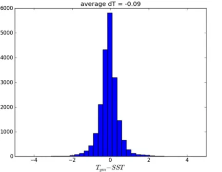
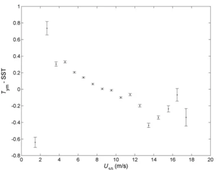
With SST the corresponding grid box mean of SOCAT’s in situ SST (generally ob-tained at 5 m nominal depth) and using all data from the years 1991 to 2007, a

his-15

togram of dT =Tym−SST was produced (Fig. 1). It shows dT was distributed around

a mean of ₋0.09 with a standard deviation of 0.55. This di_fference implied that the gridded in situ SST systematically overestimatedTym. The corresponding histogram of

our correctionfCO₂(Tym)−fCO₂ (SST) (not shown) revealed a similar distribution around

−1.12 µatm. The temperature di_fferences were found to be positive as well as negative

20

(Fig. 1). Positive dT can be a consequence of diurnal warming when the top layer heats up by solar radiation during the day. This heat is lost again during the night. Cooling of the top layer (negative dT) is a less described phenomenon but can be expected in colder environments. We found more negative dT during the winter months and at high latitudes. The temperature profile in the sea depends on wind speed as wind

25

mixes the water column, i.e. for strong winds SST is expected to be more constant in the vertical. We illustrate the wind speed dependence of dT for the North Atlantic because this region has the highest SOCAT data density. For each dT we retrieved the monthly 1◦_×1◦ grid box mean of 10 m wind speed, U10 (m s−

1

(9)

OSD

11, 1895–1948, 2014

climatology

Title Page

Tables Figures

◭ ◮

Back Close

Full Screen / Esc

Discussion

P

a

per

|

Discus

sion

P

a

per

|

Discussion

P

a

per

|

Discussion

P

a

per

|

GHG’s composite of GlobWave merged altimeter data (http://www.oceanflux-ghg.org/ Products/OceanFlux-data/Monthly-composite-datasets). A scatter plot of dT as a func-tion ofU10, averaged over in 1 m s−

1

U10 bins, (Fig. 2) showed that dT decreased with

increasingU₁₀ becoming negative for wind speeds over about 10 m s−1. Similar trends were seen in the other regions, but with dT turning negative for different wind speeds:

5

North Pacific 9 m s−1; Coastal 8 m s−1; Tropical Atlantic and Southern Ocean 6 m s−1; Tropical Pacific, Indian Ocean and Arctic 4 m s−1 (SST data from Bakker et al., 2013). The Tropical Atlantic was di_fferent in that dT became less negative for wind speed over ∼8 m s−1, turning positive over _∼10 m s−1. If only North Atlantic data from the winter months December, January and February were included, nearly all dT values would be

10

negative.

1.5 The OceanFlux climatology offCO2 and SST

We have converted the SOCAT’s instantaneousfCO₂(and SST) data to a monthly mean

fCO₂ using a climate data record of SST. This approach has only recently become

possible due to the availability of the consistently calibrated sea surface temperature

15

climate record (Merchant, 2008, 2012). In order to eliminate biases due to the sampling year (i.e., surface oceanfCO₂ has been increasing over the years)fCO₂ values from all

years were extrapolated to reference year 2010 using a simple linear relationship.

2 The SOCAT database

2.1 Introduction

20

The SOCAT database contains millions of surface ocean CO2 measurements in all

ocean areas spanning four decades. All data are put in a uniform format while clearly defined criteria are applied in their quality control. SOCAT has been made possible through the cooperation (data collection and quality control) of the international marine

(10)

OSD

11, 1895–1948, 2014

climatology

Title Page

Tables Figures

◭ ◮

Back Close

Full Screen / Esc

Discussion

P

a

per

|

Discus

sion

P

a

per

|

Discussion

P

a

per

|

Discussion

P

a

per

|

carbon science community. The history and organisation of SOCAT is described in Pfeil et al. (2013). SOCAT version 1.5 includes 6.3 million measurements from 1968 to 2007 and was made publicly available in September 2011 at http://www.socat.info/ SOCATv1/ . SOCAT data is available as three types of data products: individual cruise files, gridded products and merged synthesis data files. For our study we used the

5

latter and we downloaded the individual regional synthesis files from http://cdiac.ornl. gov/ftp/oceans/SOCATv1.5/. The content of these files (parameter names, units and descriptions) are described in Table 5 in Pfeil et al. (2013). The data can be displayed in the online Cruise Data Viewer (Fig. 3) and downloaded in text format.

2.2 The SOCAT computation of SOCAT fugacity in seawater

10

The collected CO₂concentrations are expressed as mole fraction, xCO₂, partial

pres-sure,pCO₂, or fugacity,fCO₂, of CO2. SOCAT’s re-computation is to achieve a uniform

representation of the CO2 measurements and all measurements are converted to

fu-gacity in seawaterf_CO

2,is (fCO2_rec) for in situ sea surface, SST (temp). The

parame-ters in brackets refer to their SOCAT version 1.5 names (Table 5 in Pfeil et al., 2013).

15

SST is the intake temperature which signifies SSTdepth. The shipboard measurements

were taken at equilibrator temperature T_eq (Temperature_equi) and equilibrator pres-sure, Peq (Pressure_equi). SOCAT calculates fCO₂,is from pCO₂,is, partial pressure in

seawater corrected for the difference between SST and the temperature at the equili-brator, using Eqs. (1) and (2)

20

pCO₂,is=pCO₂(Teq) exp(0.0423(SST −Teq)) (1)

fCO₂,is=pCO₂,isexp



  h

B(CO2, SST)+2(1−xCO₂,wet(Teq)) 2

δ(CO2, SST)

i Peq

R·SST





(11)

OSD

11, 1895–1948, 2014

climatology

Title Page

Tables Figures

◭ ◮

Back Close

Full Screen / Esc

Discussion

P

a

per

|

Discus

sion

P

a

per

|

Discussion

P

a

per

|

Discussion

P

a

per

|

withB(CO₂, SST) andδ(CO₂, SST) calculated from Weiss (1974):

B(CO2,T)=−1636.75+12.0408T−3.27957×10−2T2+3.16528×10−5T3 (3)

δ(CO2,T)=57.7−0.118T (4)

(Pfeil and Olsen, 2009). In Eqs. (1)–(4)fCO₂ and pCO₂ are in µatm, Peq in hPa,

tem-5

peratures are in kelvins andxCO₂,wet(Teq) is the wet mole fraction as parts per million

(ppm) of CO2 at equilibrator. The gas constant R=82.0578 cm 3

atm (mol K)−1. How

pCO₂(Teq) is measured, the temperature correction (Eq. 1) and the necessarily diff

er-ent starting points of the computation are discussed in respective Sects. 2.3–2.5. Our conversion, from the givenfCO₂,is calculated for in situ measurements to climatological

10

fCO₂,cl in 2010 is explained in Sect. 3.

2.3 Measurements ofpCO2(Teq)

The measurement method ofpCO₂ in seawater described by Takahashi et al. (2009) is

summarized in the following. On board the ship carrier gas is equilibrated with stream-ing seawater in the headspace of an equilibrator and the concentration of CO₂in the

15

equilibrated carrier gas is measured. When a dry carrier gas is analysed, seawater

pCO₂(Teq) in the equilibrator chamber is computed using

pCO₂(Teq)=xCO₂,dry(Peq−Pw) (5)

where Peq is the pressure at the equilibrator, Pw water vapour pressure at Teq and

salinity (S), andxCO₂,drythe mole fraction of CO2in dry air.Pwis calculated with

20

P_w=exp(24.4543₋67.4509(100/T_eq)₋4.8489(ln(T_eq/100)₋0.000544S) (6) withTeqin Kelvin andSthe sample salinity (Pfeil and Olsen, 2009). When mixing ratios

in a wet carrier gas (100 % humidity) are determined,Pwis set to zero

pCO₂(Teq)=xCO₂,wetPeq. (7)

(12)

OSD

11, 1895–1948, 2014

climatology

Title Page

Tables Figures

◭ ◮

Back Close

Full Screen / Esc

Discussion

P

a

per

|

Discus

sion

P

a

per

|

Discussion

P

a

per

|

Discussion

P

a

per

|

2.4 Temperature handling

There are different methods to correct for the difference in partial pressure at intake and equilibrator temperature. SOCAT uses the simple Eq. (1) (Pfeil and Olsen, 2009); they refer to more complicated methods but disregard these because they require knowl-edge of the total dissolved inorganic carbon,TCO₂, and alkalinity,TAlk, and are not

de-5

termined for isochemical conditions. Takahashi et al. (2009) use

pCO₂,is=pCO₂(Teq) exp

0.0433(SST −Teq)−4.35×10−5 SST 2

−Teq2

(8)

with SST andTeq in◦C. Equations (1) and (8) correct for the effect of slight warming

before measurement at the equilibrator on an isochemical transformation (TCO₂andTAlk

are unchanged but pH and aqueous CO₂concentration may vary). Equation (8) is an

10

integrated form of

δln(pCO₂)/δT =0.0433−8.7×10−5T

while in Eq. (1) a mean coefficient of 0.0423◦C−1 is used. Equation (8) was therefore expected to give more accuratepCO₂,is estimates.

2.5 Starting points of the SOCAT computation

15

Different measured parameters are available in different records to use as starting point for the SOCAT re-computation offCO₂,is(Table 4 in Pfeil et al., 2013). Therefore SOCAT

applies the following strict guidelines:

1. recalculatefCO₂ whenever possible;

2. order of preference of the starting point is:xCO₂,pCO₂,fCO₂;

20

(13)

OSD

11, 1895–1948, 2014

climatology

Title Page

Tables Figures

◭ ◮

Back Close

Full Screen / Esc

Discussion

P

a

per

|

Discus

sion

P

a

per

|

Discussion

P

a

per

|

Discussion

P

a

per

|

The majority of the cases (57.5 %) is derived from xCO₂,dry(Teq). However, in many

cases onlyfCO₂,is (8.4 %) orpCO₂,is(13.8 %) was provided so that it is not certain that

Eq. (1) was used by the cruise scientists to convert pCO₂(Teq) to pCO₂,is. Moreover,

if only fCO₂,is was reported, but pressure and salinity were not, fCO₂,is is not

recalcu-lated and fCO₂,is is taken as provided. The regional synthesis files only contain

re-5

computed fCO₂,is values and don’t give direct information about starting points other

than which one was used (fCO2_source). However, each record contains a field “doi”, indicating the digital object identifier to a publically accessible online data file in the PANGAEA database (http://www.pangaea.de/) where the original measurements be-fore re-computation can be found. The individual cruise data files also contain various

10

xCO₂, pCO₂, and fCO₂ data (Table 5 in Pfeil et al., 2013). Because we wanted to use

SOCAT‘s uniform database, and not re-create it, we estimatedfCO₂,cl from the fCO₂,is

values in the merged synthesis files as explained in Sect. 3. An estimation of the errors in re-computedfCO₂,cldue to varying starting points is given in Sects. 5.6 and 5.7.

3 Our re-computation for climatological fugacity in the year 2010

15

3.1 Inversion: conversion offCO2,is topCO2(Teq)

We used Eqs. (2) and (8) (with SST=Tym, i) to calculate fCO₂,ym, i but because mole

fractionxCO₂,is, and partial pressurespCO₂,isandpCO₂(Teq) are not given in the SOCAT

regional synthesis files, the first step was to estimate the original measurement of

pCO₂(Teq). FirstpCO₂,iswas derived fromfCO₂,is by inverting Eq. (2):

20

pCO₂,is=fCO₂,isexp



 −

h

B+2(1₋xCO₂,wet(Teq)) 2

δiPeq

R_· SST





 (9)

withB=B(CO2, SST) andδ=δ(CO2, SST) from Eqs. (3) and (4) and SST the SOCAT

measurement. DefiningxCO₂,wet(Teq) aspCO₂(Teq)/Peq (Eq. 7) and writingpCO₂(Teq) in

(14)

OSD

11, 1895–1948, 2014

climatology

Title Page

Tables Figures

◭ ◮

Back Close

Full Screen / Esc

Discussion

P

a

per

|

Discus

sion

P

a

per

|

Discussion

P

a

per

|

Discussion

P

a

per

|

terms ofpCO₂,is(Eq. 1), Eq. (9) leads to

pCO₂,is=fCO₂,isexp



   

−

B+21₋pCO2,isexp(−0.0423(SST_P −Teq))

eq

2 δ

Peq

R_· SST



   

. (10)

Equation (10) was solved with an iterative calculation

[pCO₂,is]n+1=fCO₂,isexp(g([pCO₂,is]n, SST,Teq,Peq)) (11)

(with g a function describing the exponent). In the first iteration the initial guess of

5

[pCO₂,is]1 was fCO₂,is and the result [pCO₂,is]2 was put back in the right hand side of

Eq. (11). This step was repeated until_|[pCO₂,is]N−[pCO₂,is]N−1|<2− 52

. Using Eq. (1) we could then estimate the originalpCO₂(Teq),

pCO₂(Teq)=pCO₂,isexp(−0.0423(SST −Teq)) (12)

3.2 Conversion ofpCO2(Teq) tofCO2,clin the year 2010

10

The next step was to convert partial pressure at equilibrator temperature to partial pres-sure atTym, ifor each SOCAT measurement. Because ARC ATSR data were available

from August 1991 we converted SOCAT data from then onwards. As a consequence 95 249 (1.4 %) of validfCO₂ observations were not used from the SOCAT v1.5 dataset

(from 119 cruises spread all over the globe). We note that the ESA CCI project is now

15

working on an extended SST climate data record from satellite extending back to 1981 which is expected in 2015. Following Takahashi et al. (2009) we used Eq. (8) to correct for the difference between climatological and equilibrator temperature

pCO₂,ym, i=pCO₂(Teq) exp

0.0433(Tym, i−Teq)−4.35×10−5 Tym, i2 −T 2 eq

(15)

OSD

11, 1895–1948, 2014

climatology

Title Page

Tables Figures

◭ ◮

Back Close

Full Screen / Esc

Discussion

P

a

per

|

Discus

sion

P

a

per

|

Discussion

P

a

per

|

Discussion

P

a

per

|

The subscript “ym” indicates a “single year monthly composite” and “i” interpolated to SOCAT sample location (Sect. 1.4). Equation (8) was applied because an isochemical transformation between SST andTym was a reasonable assumption, i.e. total carbon

and alkalinity in the ocean surface was not expected to vary significantly during one month. Next, monthly composite estimations off_CO

2,ym, iwere calculated frompCO2,ym, i

5

according to Eq. (2),

fCO₂,ym, i=pCO₂,ym, iexp



   

B+21₋pCO2_P (Teq)

eq,ym

2 δ

Peq,ym

R·Tym, i



   

(14)

withB=B(CO2,Tym, i) (Eq. 3) andδ=δ(CO2,Tym, i) (Eq. 4). We estimatedPeq,ymfrom

sea level pressure estimated at closest grid value from 6 hourly NCEP/NCAR as given in SOCAT’s merged synthesis files (ncep_slp). To account for the overpressure that is

10

normally maintained inside a ship 3 hPa was added (Peq,ym=ncep_slp+3 hPa)

(Taka-hashi et al., 2009). Note that we recomputed SOCAT’sfCO₂ for monthly composite SST

and atmospheric pressure, but not for monthly composite salinity. However, if in situ salinity was not provided by the investigator, SOCAT used a monthly composite sea surface salinity from the World Ocean Atlas 2005 (woa_sss) for their computation of

15

fCO₂,is. The consequences of missing salinity values are assessed in Sect. 5.7. For all

yearspCO₂,ym, iandfCO₂,ym, iwere extrapolated to the year 2010, producingpCO₂,cl, iand

fCO₂,cl, i referenced to 2010, using the same mean rate of change (1.5±0.3 µatm yr− 1

) as Takahashi et al. (2009) used forpCO₂. Takahashi et al. (2009) extrapolate to the year

2000, so if the rate of change has increased since then ours could be a low estimate.

20

Finally, thefCO₂,cl, iandpCO₂,cl, idata were grouped by month and averaged over 1◦×1◦

squares. Not all 1◦×1◦grid boxes were filled and we horizontally interpolated between filled values to produce globalpCO₂,clandfCO₂,cl distributions (Sect. 4).

(16)

OSD

11, 1895–1948, 2014

climatology

Title Page

Tables Figures

◭ ◮

Back Close

Full Screen / Esc

Discussion

P

a

per

|

Discus

sion

P

a

per

|

Discussion

P

a

per

|

Discussion

P

a

per

|

3.3 Missing values

We dealt with missing SOCAT variables following Pfeil and Olsen (2009):

1. we only used “good” records (WOCE_flag=2); 2. we only used records with validfCO₂,isand SST;

3. ifTeq was invalid we used SST;

5

4. ifPeq was invalid we used atmospheric pressure,Patm,+3 hPa;

5. ifPeq andPatm were invalid we used ncep_slp+3 hPa.

4 Horizontal extrapolation using ordinary block kriging

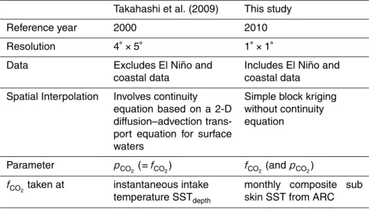
Unlike Takahashi et al. (2009), our climatology includes data from El Niño years and coastal locations. We addedp_CO

2,clfor those who prefer to use partial pressure;pCO2,cl

10

levels were slightly higher (less than 2 µatm) thanfCO₂,cl. For the spatial interpolation of

the gridded data on a 1◦_×1◦ mask map of the global oceans we used gstat, an open source computer code for multivariable geostatistical modelling, prediction and simula-tion (gstat home page: http://www.gstat.org/). Gstat finds the best linear unbiased pre-diction (the expected value) with its prepre-diction error for a variable at a location, given

15

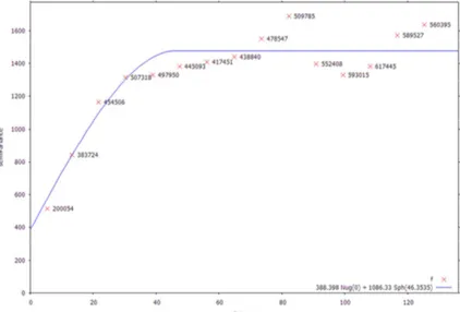
observations and a model for their spatial variation (Pebesma, 1999). We quantified the prediction error as standard deviation (square root of the variance given by gstat). First, we modelled the variogram for fCO₂,cl for each month using gstat’s interactive

user interface (Pebesma, 1999). A variogram describes how the data varies spatially and can be represented by a plot of semivariance against distance. The variograms

20

(17)

OSD

11, 1895–1948, 2014

climatology

Title Page

Tables Figures

◭ ◮

Back Close

Full Screen / Esc

Discussion

P

a

per

|

Discus

sion

P

a

per

|

Discussion

P

a

per

|

Discussion

P

a

per

|

used the same variogram as forfCO₂,clbecause the difference withfCO₂,clwas negligible

compared to the spatial variation.

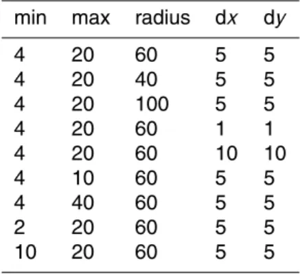
We applied ordinary kriging on mask map locations because it is the default ac-tion when observaac-tions, variogram, and predicac-tion locaac-tions are specified (Pebesma, 1999). We performed local ordinary block kriging on a 1◦×1◦ mask map of the global

5

oceans with min=4, max=20, and radius=60. Thus, after selecting all data points at (euclidian) distances from the prediction location less or equal to 60, the 20 clos-est were chosen when more than 20 were found and a missing value was generated if less than 4 points were found. The data were smoothed by averaging over square shaped 5_×5 sized blocks. Thus gstat produced thef_CO

2,cl(andpCO2,cl) prediction and

10

variance values located at the grid cell centres of the (non-missing valued) cells in the grid map mask. These results were compared with results from different kriging options min, max, radius and block size (Sect. 5.3).

Our approach was simpler than the spatial interpolation on a 4◦_×5◦grid of Takahashi et al. (2009). For each day they increase pixel size to four neighbouring pixels over

15

3 days (past, present and future day). The values of the pixels that are still without observations after this procedure are computed by a continuity equation based on a 2-D diffusion–advection transport equation for surface waters. All daily pixel values are used to calculate monthly mean values. Takahashi et al. (2009) estimate that the global mean surface waterpCO₂,clobtained in their study may be biased by about+1.3 µatm

20

due to under sampling and the interpolation method. The spatial interpolation method we applied is expected to give unbiased results (Pebesma, 1999).

5 Results

5.1 Monthly global maps

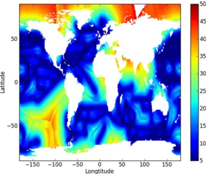
The prediction distributions offCO₂,clproduced by the ordinary block kriging are shown

25

in Fig. 5 for all 12 months. The maps showing the standard deviations of the kriging

(18)

OSD

11, 1895–1948, 2014

climatology

Title Page

Tables Figures

◭ ◮

Back Close

Full Screen / Esc

Discussion

P

a

per

|

Discus

sion

P

a

per

|

Discussion

P

a

per

|

Discussion

P

a

per

|

for January (all months) are show in Fig. 6 (Fig. A1). The 12 monthly global distri-bution data have been made available in 12 netCDF-3 files in the Supplement re-lated to this article. These files contain fCO₂,cl, pCO₂,cl, their spatial interpolation

er-rors, and ARC’s SSTskin for the year 2010, all on a 1◦×1◦ grid. The variable names

are respectively fCO2_2010_krig_pred, pCO2_2010_krig_pred, fCO2_2010_krig_std,

5

pCO2_2010_krig_std, and Tcl_2010 (Tym as defined in Sect. 1.4 for the year 2010).

Monthly gridded values of atmospheric CO2dry air mole fractions in 2010, made

avail-able by the NOAA ESRL Carbon Cycle Cooperative Global Air Sampling Network (Dlu-gokencky et al., 2014), are also given as variable vCO2_2010. These were not used in our conversion but can help calculate air-sea gas CO2 fluxes (Takahashi, 2009). The

10

important differences with the Takahashi climatology are summarized in Table 1. A range of errors needs to be considered when interpreting the final monthly maps. It is difficult to be complete but we considered the following errors. The spatial interpo-lation errors were estimated by taking the square root of the variances of the kriging. The different kriging approaches themselves were evaluated by calculating the mean

15

and standard deviations of the varying fCO₂,cl kriging results using the options shown

in Table 2. The cruises were bootstrapped to investigate if certain cruises dominated the mapped results. Other errors that were analysed were the “temporal extrapolation error”, the “inversion error” related to the different starting points, the consequences of the missing values, and the propagations of the uncertainties in the SOCAT

measure-20

ments andTym, i. These errors are discussed in the next sub sections and the final sub

section gives a summary overview.

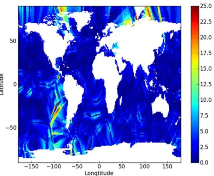
5.2 Spatial interpolation errors

The standard deviations (SD) of the applied kriging were calculated by taking the square root of the variance values produced by gstat (Pebesma, 1999). Kriging errors

25

were obviously related to the available SOCAT data density in the measurement month (e.g., Fig. 3). ThefCO₂,cl kriging SD mapped for all months are illustrated in Fig. A1.

(19)

OSD

11, 1895–1948, 2014

climatology

Title Page

Tables Figures

◭ ◮

Back Close

Full Screen / Esc

Discussion

P

a

per

|

Discus

sion

P

a

per

|

Discussion

P

a

per

|

Discussion

P

a

per

|

means_±Sd). The average monthly minimum and maximum SD values were 6.3_±2.6 and 50±8.7 µatm. Problem areas emerged where no SOCAT data were available, for example in the western Southern Ocean and the Arctic. Spatial interpolation errors were lowest in the North Atlantic and North Pacific where SOCAT data was dense. The month April showed the highest errors, this could be a consequence of the

vari-5

ogram range,c, being the smallest (implying that the covariance between the locations dropped quickly with distance). Our variogram model of combination of a nugget and a spherical model did not fit November data well as the semivariance was almost inde-pendent of distance; the low standard deviations in November (Fig. A1) were therefore probably not representative of the true error due to the kriging method. Standard

devi-10

ations of the kriging are included in our presented data files; a bias is not supposed to be introduced by the kriging itself (Pebesma, 1999).

5.3 A comparison of the different kriging approaches

The ordinary block kriging of thef_CO

2,cl data was repeated using a range of sensible

kriging parameters (Table 2). The standard deviation of the mean over the different

15

kriging results (Figs. 7 and A2) was less than 5 µatm in most places, with higher values seen near the coasts, Arctic, and the western Tropical Pacific and Southern Ocean. These standard deviations were considerably smaller than those of the kriging itself (Figs. 6 and A1) but could be significant in a few places especially, but not exclusively, in the Arctic and coastal regions.

20

5.4 Are some cruises more important than others?

It was conceivable that certain cruises dominated the final results. This possibility was studied using the bootstrap method, a statistical technique which permits the assess-ment of variability in an estimate using just the available data (Wilmott et al., 1985). Bootstrapping creates synthetic sets of data by random resampling from the original

25

data with replacement. We bootstrapped the SOCAT data 10 times by cruise ID to

(20)

OSD

11, 1895–1948, 2014

climatology

Title Page

Tables Figures

◭ ◮

Back Close

Full Screen / Esc

Discussion

P

a

per

|

Discus

sion

P

a

per

|

Discussion

P

a

per

|

Discussion

P

a

per

|

estimate the variability of the mean monthlyfCO₂,cl distributions. The complete SOCAT

data set was too big to bootstrap at once. We therefore bootstrapped in two steps, first by cruise ID for each year and region, and then by year and region. Each of the 10 resulting fCO₂,cl datasets were kriged as described in Sect. 4 (for each month in

each synthetic dataset a different variogram model was fitted and applied). The mean

5

monthly distributions showed that in regions of fewer cruises (outside the North Atlantic and North Pacific) significant variation inf_CO

2,cl, could occur, with up to 50 µatm

stan-dard deviation (Figs. 8 and A3). It was therefore likely that certain cruises were indeed more important than others. High variability in the east-central equatorial Pacific could be a consequence of not excluding the El Nino years.

10

5.5 Temporal extrapolation error

The 1.5 µatm yr−1rate of change inpCO₂ has an estimated precision of±0.3 µatm yr− 1

(Takahashi et al., 2009) and ∆fCO₂,cl= ∆pCO₂,cl (Eq. 14). The error in fCO₂,cl

in 2010 due to uncertainty of the p_CO

2,cl trend was therefore estimated as

±(2010₋year)_·0.3 µatm yr−1, ranging between _±(0.9–5.7) µatm. These extrapolation

15

errors for the month of January and for all months are shown in respective Fig. 9 and Fig. A4. The error was on the high side in the Indian Ocean and in the western South-ern Ocean because fewer cruises were performed there in recent times. The absolute monthly mean extrapolation error over all grid points was estimated at 3±0.1 µatm (average over all monthly means_±standard deviation). This implies that if in reality the

20

rate of change since 1991 was 1.8 instead of 1.5 µatm yr−1,fCO₂,cl would be

underes-timated by∼3 µatm on average. Recent research has shown that this is probable, as Takahashi et al. (2014) present an updated oceanicpCO₂trend of 1.9 µatm yr−

1

(21)

OSD

11, 1895–1948, 2014

climatology

Title Page

Tables Figures

◭ ◮

Back Close

Full Screen / Esc

Discussion

P

a

per

|

Discus

sion

P

a

per

|

Discussion

P

a

per

|

Discussion

P

a

per

|

5.6 Inversion error

Our conversion offCO₂,istopCO₂(Teq) could introduce an error if the data was not based

onxCO₂ analysis (cruise flags not A or B), but onfCO₂ calculated from a

spectropho-tometer, or if the investigator only provided fCO₂,is or pCO₂,is and did not use Eq. (1)

to correct for the temperature difference. This error was assessed by calculating the

5

conversion fromfCO₂,is tofCO₂,ym, i using SST and Peq instead of Tym and Peq, ym. This

conversion would ideally produce the original SOCAT fCO₂,is value. A difference

be-tween fCO₂,is and “fCO₂,ym,i=is” implied that our re-computation differed from the one

applied by SOCAT or the investigator and we called this difference averaged over one grid box “inversion error”. Note that∆fCO₂,cl= ∆fCO₂,ym. This error turned out in a very

10

small positive bias, negligible in the North Atlantic and other areas with some higher levels in the Southern Ocean (Figs. 10 and A5). The monthly mean inversion bias over all grid points was 1_±0.2 µatm (average over all monthly means_±standard deviation).

5.7 Missing values

A related problem was introduced by missing SOCAT values (Sect. 3.3). Missing

val-15

ues did not always propagate into an inversion error because we made an effort to handle the missing values following SOCAT (Pfeil and Olsen, 2009). If salinity or pres-sure were missing, SOCAT used EO values for their conversion, reducing systematic

fCO₂,cl errors in our re-conversion. Missing values of temperature and pressure at the

equilibrator could introduce systematic errors, however. It is difficult to estimate the size

20

of these kinds of errors, but Fig. 11 shows the proportion of missing values for January to give an idea about how many data could be affected. ThefCO₂,ym, icalculations were

most sensitive to temperature. IfTeq was not provided we used in situ SST, so an

in-version error would be near zero. However, in these casespCO₂,iswas then the starting

point of our conversion instead ofpCO₂(Teq) which could lead to significant systematic

25

fCO₂,ym, i errors. We therefore also reproduced our fCO₂,cl distribution maps using only

data points with valid Teq values (Figs. 12 and A6). These maps appeared to reveal

(22)

OSD

11, 1895–1948, 2014

climatology

Title Page

Tables Figures

◭ ◮

Back Close

Full Screen / Esc

Discussion

P

a

per

|

Discus

sion

P

a

per

|

Discussion

P

a

per

|

Discussion

P

a

per

|

less highfCO₂,cl outliers. If only data with validTeq were selected the data quality was

believed to be better, but the number of data points was compromised. The monthly distributions of these data (Fig. A7) therefore showed either lower or higher SD levels. The monthly mean difference fCO₂,cl(all)−fCO₂,cl(validTeq) ranged between −3.3 µatm

(November) and 3.7 µatm (January) and was−0.4 µatm on average. The error due to

5

missing values in a monthly distribution file could therefore be interpreted as smaller than about_±3.5 µatm, resulting in a bias of the annual mean of₋0.4 µatm.

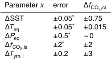
5.8 Measurement errors

Errors in the SOCAT measurements (fCO₂,is, Teq, Peq and SST) naturally propagated

intofCO₂,cl uncertainty. The accuracies for the SOCAT measurements that comply with

10

SOP (Standard Operating Procedures) criteria are given by Pfeil et al. (2013); not all SOCAT data are of this high standard so these accuracies were the highest that could be expected. Likewise the uncertainty in Tym, i had to be taken into account.

Ocean-flux GHG gives the SD values and counts with the mean SST_skin values from ARC on a 1◦×1◦grid; the average standard error (SD/√count) over all monthly grid boxes that

15

hadfCO₂ values (all years and months) was ±0.17. The uncertainty in the SST diff

er-ence with subskin SST is_±0.1 (Donlon et al., 1999). The total uncertainty inT_{ym, i}was

therefore estimated to be_±0.2 (p0.172₊_0.12_{). We estimated the propagation of these}

errors by applying the error for each parameter,x, and calculatefCO₂,cl. (We calculated

fCO₂,clforx+∆xandx−∆xand∆fCO₂,cl= mean{(fCO₂,cl(x+ ∆x)−fCO₂,cl(x−∆x))/2}.

20

The results are listed in Table 3. The total error caused by known uncertainties in the parameters was estimated to be>3.7 µatm (p0.752₊_0.0152₊₂2₊₃2_).

5.9 Summary of errors

The standard deviations of the kriging should account for both spatial variation of the data points and random errors in the fCO₂,cl values. The errors caused by the

(23)

OSD

11, 1895–1948, 2014

climatology

Title Page

Tables Figures

◭ ◮

Back Close

Full Screen / Esc

Discussion

P

a

per

|

Discus

sion

P

a

per

|

Discussion

P

a

per

|

Discussion

P

a

per

|

uncertainty of the rate of pCO₂ change (temporal extrapolation error), missing

val-ues and measurement errors are of the latter kind. Their monthly averages were estimated at 3, 3.5 and 3.7 µatm respectively and hence we could explain 5.9 µatm (p32₊_3.52₊_3.72_{) of the about 20 µatm monthly average SD of the fit. Note that an}

error of 5.9 µatm agrees well with the average monthly minimum SD of the kriging of

5

6.3±2.6 µatm, leaving some room for unexplained errors (Sect. 5.2). The above analy-sis shows that the SD of the kriging was dominated by the spatial variation of the data, closely linked to data density.

We estimated a bias of ∼1 µatm, introduced by the inversion step in the fCO₂,is to

fCO₂,ym, i conversion. The mean fCO₂,cl over all months had a bias of −0.4 µatm due

10

to missing SOCAT values in the re-computation, so for the total bias of an annual average fCO₂,cl we estimated a value between 0.6 and 1 µatm. This is less than the

systematic bias in the mean surface water pCO₂ of about 1.3 µatm as estimated by

Takahashi et al. (2009) due to under sampling and their interpolation. If we also account for a 3 µatm underestimation of the oceanicpCO₂ trend, the bias would range between

15

−2.4 and₋2 µatm.

6 SOCAT version 2

Recently, on 4 June 2013, the updated database SOCAT version 2 was released con-taining 10.1 million surface waterfCO₂values (Bakker et al., 2013). The added data are

from cruises during the years 2008 to 2011, from the Arctic, and previously unpublished

20

data from earlier cruises; also the quality control is improved. The addition of SOCAT data points and the omission of bad and questionable data gave smoother global dis-tributions (Fig. 13) and smaller kriging errors (Fig. A8). The monthly average of the SD of the kriging was 17±3 µatm (was 20±5 µatm for version 1.5). The monthly mean differencefCO₂,cl(v1.5)−fCO₂,cl(v2) ranged between−1.1 µatm (January) and 2.4 µatm

25

(July) and was 0.3 µatm on average. Our re-processed SOCAT version 2 data has also been made available.

(24)

OSD

11, 1895–1948, 2014

climatology

Title Page

Tables Figures

◭ ◮

Back Close

Full Screen / Esc

Discussion

P

a

per

|

Discus

sion

P

a

per

|

Discussion

P

a

per

|

Discussion

P

a

per

|

7 Conclusions

SOCATfCO₂ (andpCO₂) predictions and standard deviations for a reference year 2010,

recomputed for a SST suitable for climate change research of air–sea gas exchange and interpolated to a global 1◦_×1◦ grid, have been made available. Two climatology datasets are presented as an online Supplement to this paper, each consisting of

5

12 monthly NetCDF files: one using all SOCATv1.5 data and one using all data of the recent update SOCATv2. We identified and calculated various possible errors. The errors due to the spatial interpolation, closely related to data density, dominated and some areas showed higher errors of all kinds than others. The data quality/density in the North Atlantic and North Pacific proved to be superior. Our dataset based on

SO-10

CAT version 2 is mostly similar to the one based on version 1.5, but if it is used to focus on outliers version 2 should be used because the data quality is better. For future SOCAT versions: it would benefit climatological applications if additional climatological values offCO₂were directly calculated using the difference between the temperature of

sea water in the equilibrator and monthly composite temperatures such as from ARC

15

(Eq. 13), so to avoid the inversion step.

The Supplement related to this article is available online at doi:10.5194/osd-11-1895-2014-supplement.

Acknowledgements. This research is a contribution of the National Centre for Earth Observa-tion, a NERC Collaborative Centre and was supported by the European Space Agency (ESA)

20

(25)

OSD

11, 1895–1948, 2014

climatology

Title Page

Tables Figures

◭ ◮

Back Close

Full Screen / Esc

Discussion

P

a

per

|

Discus

sion

P

a

per

|

Discussion

P

a

per

|

Discussion

P

a

per

|

References

Bakker, D. C. E., Pfeil, B., Smith, K., Hankin, S., Olsen, A., Alin, S. R., Cosca, C., Harasawa, S., Kozyr, A., Nojiri, Y., O’Brien, K. M., Schuster, U., Telszewski, M., Tilbrook, B., Wada, C., Akl, J., Barbero, L., Bates, N. R., Boutin, J., Bozec, Y., Cai, W.-J., Castle, R. D., Chavez, F. P., Chen, L., Chierici, M., Currie, K., de Baar, H. J. W., Evans, W., Feely, R. A., Fransson, A.,

5

Gao, Z., Hales, B., Hardman-Mountford, N. J., Hoppema, M., Huang, W.-J., Hunt, C. W., Huss, B., Ichikawa, T., Johannessen, T., Jones, E. M., Jones, S. D., Jutterström, S., Kitidis, V., Körtzinger, A., Landschützer, P., Lauvset, S. K., Lefèvre, N., Manke, A. B., Mathis, J. T., Merlivat, L., Metzl, N., Murata, A., Newberger, T., Omar, A. M., Ono, T., Park, G.-H., Pater-son, K., Pierrot, D., Ríos, A. F., Sabine, C. L., Saito, S., Salisbury, J., Sarma, V. V. S. S.,

10

Schlitzer, R., Sieger, R., Skjelvan, I., Steinhoff, T., Sullivan, K. F., Sun, H., Sutton, A. J., Suzuki, T., Sweeney, C., Takahashi, T., Tjiputra, J., Tsurushima, N., van Heuven, S. M. A. C., Vandemark, D., Vlahos, P., Wallace, D. W. R., Wanninkhof, R., and Watson, A. J.: An up-date to the Surface Ocean CO₂ Atlas (SOCAT version 2), Earth Syst. Sci. Data, 6, 69–90, doi:10.5194/essd-6-69-2014, 2014.

15

Dlugokencky, E. J., Masarie, K. A., Lang, P. M., and Tans, P. P.: NOAA Greenhouse Gas Refer-ence from Atmospheric Carbon Dioxide Dry Air Mole Fractions from the NOAA ESRL Carbon Cycle Cooperative Global Air Sampling Network, available at: ftp://aftp.cmdl.noaa.gov/data/ trace_gases/co2/flask/surface/ (last access: 27 July 2014), 2014.

Donlon, C. J., Nightingale, P. D., Sheasby, T., Turner, J., Robinson, I. S., and Emery, J.:

Implica-20

tions of the oceanic thermal skin temperature deviation at high wind speeds, Geophys. Res. Lett., 26, 2505–2508, 1999.

Donlon, C. J., Minnett, P., Gentemann, C., Nightingale, T. J., Barton, I. J., Ward, B., and Mur-ray, J.: Towards improved validation of satellite sea surface skin temperature measurements for climate research, J. Climate, 15, 353–369, 2002.

25

Donlon, C., Robinson, I., Casey, K. S., Vazquez-Cuervo, J., Armstrong, E., Arino, O., Gente-mann, C., May, D., Leborgne, P., Piollé, J., Barton, I., Beggs, H., Poulter, D. J. S., Merchant, C. J., Bingham, A., Heinz, S., Harris, A., Wick, G., Emery, B., Minnett, P., Evans, R., Llewwellyn-Jones, D., Mutlow, C., Reynolds, R. W., Kawamura, H., and Rayner, N.: The GODAE High Resolution Sea Surface Temperature Pilot Project (GHRSST-PP), B. Am. Meteorol. Soc., 88,

30

1197–1213, 2007.