www.atmos-meas-tech.net/8/2051/2015/ doi:10.5194/amt-8-2051-2015
© Author(s) 2015. CC Attribution 3.0 License.
Methodology for determining multilayered temperature inversions
G. J. Fochesatto
Department of Atmospheric Sciences, Geophysical Institute and College of Natural Science and Mathematics, University of Alaska Fairbanks, 903 Koyukuk Dr., Fairbanks, Alaska 99775, USA
Correspondence to:G. J. Fochesatto (foch@gi.alaska.edu)
Received: 6 September 2014 – Published in Atmos. Meas. Tech. Discuss.: 16 October 2014 Revised: 7 April 2015 – Accepted: 8 April 2015 – Published: 11 May 2015
Abstract.Temperature sounding of the atmospheric bound-ary layer (ABL) and lower troposphere exhibits multilayered temperature inversions specially in high latitudes during ex-treme winters. These temperature inversion layers are origi-nated based on the combined forcing of local- and large-scale synoptic meteorology. At the local scale, the thermal inver-sion layer forms near the surface and plays a central role in controlling the surface radiative cooling and air pollution dis-persion; however, depending upon the large-scale synoptic meteorological forcing, an upper level thermal inversion can also exist topping the local ABL.
In this article a numerical methodology is reported to de-termine thermal inversion layers present in a given tempera-ture profile and deduce some of their thermodynamic prop-erties.
The algorithm extracts from the temperature profile the most important temperature variations defining thermal in-version layers. This is accomplished by a linear interpola-tion funcinterpola-tion of variable length that minimizes an error func-tion. The algorithm functionality is demonstrated on actual radiosonde profiles to deduce the multilayered temperature inversion structure with an error fraction set independently.
1 Introduction
The atmospheric boundary layer (ABL) is the lowest part of the troposphere in permanent contact with the earth surface and responds to thermal and roughness surface forcing in timescales of minutes to hours (Stull, 1988). Synoptic large-scale meteorological processes condition the ABL state by driving relatively rapid horizontal air mass exchange for ex-ample under a cyclonic air mass advection (Fochesatto et al., 2002) or simply by imposing, on upper tropospheric levels,
an adiabatic compression through the formation of a high-pressure anticyclone (Byers and Starr 1941; Bowling et al., 1968; Curry, 1983; Cassano et al., 2011). These large-scale synoptic processes constrain the temperature of the air mass in tropospheric levels without initial connection to the local surface temperature forming vertically localized positive up-ward thermal gradients called elevated inversion (EI) layers (Csanady, 1974; Milionis and Davies, 1992, 2008; Mayfield and Fochesatto, 2013).
Although the ABL timescale for surface response ranges from minutes to hours (Garrat and Brost, 1981; Stull, 1988), the ABL response to synoptic forcing at local scale initiated by the radiative and dynamic interaction in the presence of the EIs can vary from hours to several days depending on a number of factors related to topographic conditions, temper-ature and wind distribution, thermal stratification and synop-tic air mass type (e.g., moist cyclone advection or dry ansynop-ticy- anticy-clone situations, Mayfield and Fochesatto, 2013).
pools Mahrt et al., 2001; Clements et al., 2003; Whiteman and Zhong, 2008; Fochesatto et al., 2013). Of particular in-terest is the formation and breakup of the SBI layer (Billelo, 1966; Hartman and Wendler, 2005), its thermal regime across time as it forms (i.e., fast cooling at the formation process fol-lowed by a growing depth phase) (Malingowski et al., 2014) and its thermodynamic characteristics controlling the sensi-ble and latent heat exchange rate (Raddatz et al., 2013a, b). Moreover, simultaneous determination and characterization of EI layers and SBI has the potential to improve assess-ment on local air pollution meteorology (André and Mahrt, 1982), to improve forecasting of freezing rain episodes (Rob-bins and Cortinas, 2002), to determine heat exchanges in un-consolidated sea-ice surfaces (Raddatz et al., 2013 a, b) and potential impact on subarctic and Arctic climate (Ueno et al., 2005; Eastman and Warren, 2010; Bintanja et al., 2011).
The most widely used instrumentation to observe thermal inversion layers is direct temperature determination by high-resolution radiosondes. However the methodologies to ana-lyze the radiosonde temperature profile (see for example Sei-del et al., 2010) still do not account for complex embedded thermal structures. On the other hand some authors have clas-sified these layers as being short-living structures and there-fore discarded from their analyses (Kahl 1990; Serreze et al., 1992). However, it was recently demonstrated during the Winter Boundary-Layer Experiment (Wi-BLEx) (Fochesatto et al., 2013; Mayfield and Fochesatto, 2013; Malingowski et al., 2014) that complex thermal structures persist with some changes through the day depending on environmental condi-tions.
Nonetheless, trying to detail more in-depth turbulent mix-ing processes in the ABL, the observations demand instru-mentation that can profile the atmosphere at higher spatial and temporal resolution than what a radiosonde instrument can provide. Thus active remote sensing instruments give a better description of the vertical structure and dynamics of the ABL such as the case for example of lidar (Light Detec-tion And Ranging, Fochesatto et al., 2001a, b, 2004, 2005, 2006) and sodar (SOund Detection And Ranging; Beyrich and Weill, 1993; Fochesatto et al., 2013). Particularly inter-esting is the high temporal and spatial resolution at which li-dars can describe the initiation of convection close to the sur-face as well as the dynamic of the residual layer (Fochesatto et al., 2001 a, b). Similarly, insightful description of the tur-bulent and dynamic structure of the ABL when shallow cold flows penetrate the stable ABL can be gained by using sodar profilers (Fochesatto et al., 2013). On the other hand, pas-sive ground-based remote sensors i.e., microwave radiome-ters, based on background sky microwave radiation sensing are another option to profile the ABL at ∼minute resolution. Methodologies to determine the ABL height using lidars are based on detecting the changes in the optical backscatter-ing level when the laser beam crosses the interface between the air mass in the ABL and the free troposphere (Menut et al., 1999; Bianco and Wilczak, 2002; Brooks, 2003;
Lam-mert and Bosenberg, 2006). However, determining the ABL height using sodar becomes a little more complicated be-cause the observations give access to the temperature struc-ture of turbulenceCT2 profile that changes depending upon the ABL phase, terrain and multilayer structure (Holmgren et al., 1975; Beyrich and Weill, 1993).
Radiosonde determination of thermal inversion layers to study the Arctic Ocean ABL has been done using function fit-ting on radiosonde in the Arctic Ocean (Serreze et al., 1992) to determine the large-scale climate signature in the SBI time series of polar regions of the Arctic and Antarctic (Seidel et al., 2010; Zhang and Seidel, 2011; Zhang et al., 2011). In short-term studies, Khal (1990) and Khal et al. (1992) imple-mented a methodology to explore the temperature profile and then, applying some constraints, deduce the SBI top height, using similar methodologies trying to link time series of SBI heights to large-scale climate processes in continental Alaska (Bourne et al., 2010).
In this article a mathematical procedure is described, and its numerical implementation is documented to determine the multilayer thermal structure present on a given temper-ature profile in the lower troposphere. Section 2 describes the mathematical procedure and numerical implementation, Sect. 3 determines the calibration factor, Sect. 4 applies the numerical procedure to routine and high-resolution ra-diosonde observations and Sect. 5 gives a final assessment of the implemented numerical methodology.
2 Methodology
A thermal inversion layer represents a region in the atmo-sphere defining a positive upward temperature gradientddTz >
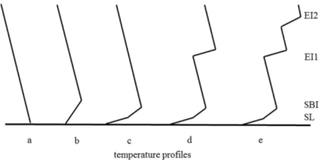
0, whereT is the temperature andz is the height. As de-scribed in the Introduction this positive upward temperature gradient can have two origins: the first one related to sur-face cooling (i.e., sursur-face net radiation loss) giving origin to the formation of the so-called SBI, and the second one orig-inated after synoptic large-scale processes (i.e., upper level warming also known as EI layers) (Mayfield and Fochesatto, 2013). Under these conditions the temperature profile in the lower troposphere is expected to describe either a neutral thermal condition (no inversion present), isothermal layers, presence of a surface-based inversion (SBI), development of stratified layers within the SBI layer depth, shallow inversion layers above the SBI inversion top or more complex situa-tions in which upper-level thermal inversions are also present with base and top in the outflow ABL (Khal, 1990; Mayfield and Fochesatto, 2013). Figure 1 depicts the more relevant sit-uations.
func-Figure 1. Illustration of temperature profiles indicating different thermodynamics conditions from left to right: (a) no inversion present;(b) presence of an SBI;(c)presence of a stratified SBI; (d)SBI stratified in the presence of an EI and(e)SBI stratified and multiple EIs. Modified after Khal (1990).
tion calculated on the basis of an iterative linear interpola-tion routine. The numerical routine is based on fitting and refitting a piecewise linear interpolating function with vari-able length to define layer by layer the temperature profile composition. An error quote controls the algorithm conver-gence by layer and is calculated based on the largest singular valueεby which thermal features in the temperature profile can be reproduced. The numerical method actually reduces the number of points present in the original temperature pro-file. Therefore after applying the numerical methodology, the temperature profile became a data structure defining thermo-dynamic characteristics of thermal layers found in the tem-perature profile. Further on, exploring the data structure we can define a thermal inversion layer as the layer in which the temperature gradient turns positive upward to negative up-ward.
Equation (1) indicates the mathematical formula describ-ing the piecewise linear approximation of the temperature profile:
φ (z)= N−X1
k=1
mk.z+bk, (1)
wherek represents each linear interval fitting and N is the total number of temperature measurements. The sequence of linear fitting is executed by selecting two temperature points at the time – one from the top height and the other from bot-tom height maintaining botbot-tom fixed – until the linear piece-wise function minimizes the error quote against the tempera-ture profile as indicated in Eq. (2):
ε= kφ (z)−T (z)k. (2) Hereεrepresents the mathematicalnormorEuclidean dis-tancebetween the linear piecewise mathematical representa-tionφ (z)and the original temperature profileT (z).
This way the temperature profile is assimilated to the se-ries of sequentially fitted linear intervals defining the tem-perature function. It has to be noted that after the layer (k)
has been detected, the layer (k+1) considers its lowermost point as being the top height of layer (k)and starts over again “connecting” this point with the top-height point of the tem-perature profile and, from there, descending in height until theεvalue reaches the preset threshold. This way the proce-dure continues until the entire temperature profile has been scanned and assimilated to frames defined by piecewise lin-ear functions.
Basically the number of piecewise linear functions (k)
will be defined by the ultimate number of temperature measurements composing the temperature profile (N ); thus max(k)=N−1. However, increasing the error fraction (ε)
will therefore reduce the max(k)reached. In such a case the final approximation formula is expressed in Eq. (3):
φ (z)= k=p X
k=1
mk.z+bk, (3)
wherepis the total number of points from the original tem-perature profile that has been retained by the fitting process.
Table 1 indicates a five-layer temperature structure in the ABL up to 1 km height based on six-point temperature sim-ulation. The profile defines a stratified SBI with top height at 250 m topped by an EI at 670 m. Figure 2 illustrates the se-quences in which the algorithm operates to search and define each layer from 1 to 5. In this case we retain all points in the temperature profile.
3 Convergence factor
Since the ability of the algorithm to extract thermal inversion layers depends upon the value chosen forε, then it is reason-able to determine for example what threshold value of tem-perature profile gradient dT /dzin◦C/100 m can be retrieved when a given value ofεis preset. To deduce this relationship a numerical simulation was performed scanning values ofε
from 0.1 to 20 over a temperature profile displaying a single thermal inversion which was varied in temperature strength
1T from 0.1 to 20◦C and vertical depth1zfrom 1 to 500 m. For each step onεvalues the temperature gradient threshold dT /dz, able to determine that specific layer, was deduced.
Figure 3 panel on the left illustrates the simulated tem-perature inversion and the applied temtem-perature strength and vertical depth variability. Similarly the temperature gradient threshold as a function of the convergence errorεis shown in Fig. 3 in the panel on the right. This relationship was deter-mined in an ideal scenario of a single temperature inversion layer. Following Fig. 3 (right panel), if a constant inversion layer depth is analyzed (e.g.,1z=200 m) and starting on
Table 1.Proposed thermal layers in a temperature profile.
Layer 1 2 3 4 5 Units
Tt,zt −20, 100 −15, 250 −22, 550 −17, 670 −23, 1000 ◦C, m
Tb,zb −30, 0 −20, 100 −15,−22 −22, 550 −17, 670 ◦C, m dT /dz 10 3.3 −2.3 4.2 −1.8 ◦C/100 m
Class – – SBI – EI
Figure 3.Convergence error simulation: the left panel illustrates the simulated temperature inversion varying1Z in meters and1T in degrees Celsius. Right panel is the minimum thermal gradient detected expressed in◦C/100 m on a single inversion layer as function of the preset errornormεvarying from 0.1 to 20. The parameter in this curve is the layer depth represented in this case from 1 to 200 m.
or less sensitivity to detect thermal structures present in the given temperature profile.
4 Numerical application
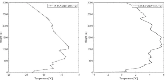
In this section the numerical method is applied to the resti-tution of thermal layers from radiosonde data. Two cases are examined. The first one comes from the radiosonde data archive of NOAA-ESRL database for the Fairbanks Inter-national airport WMO station code 70261 retrieved from the Wyoming radiosonde database (http://weather.uwyo.edu/ upperair/sounding.html). The sounding was taken on 15 Jan-uary 2014 at 00:00 UTC (Fig. 4 – left panel). The second case corresponds to one of the GPS sounding cases taken during an intensive observing period in the framework of Wi-BLEx (Malingowski et al., 2014). In this case a morning sounding was chosen during 13 October 2009 at 15:00 UTC (Fig. 4 – right panel) during formation process of the SBI layer.
Table 2 summarizes all retrieved layers extracted preset-ting ε=0.1. This setting allowed detecting p=24 layers over 32 temperature points below 3 km in the case of 15 January 2014 at 00:00 UTC, while for 13 October 2009 at 15:00 UTC the sounding presents 677 points below 3 km and
p=56 layers were detected.
From the analysis of detected layers one can initially search in the data structure the changes in mk.mk> 0 will be assigned to positive upward dT /dz, while negative will indicate the opposite. From the analysis of the resulting data it can be deduced that the inversion layer, defined whenmk changes from positive to negative, will be assigned as SBI
when the base of that inversion is located at the surface, re-gardless of its stratification condition, while, on the other hand, any other inversion layer with base off the ground will be called EI. In the case of 15 January 2014 at 00:00 UTC, it was found that the SBI top height is located at 165 m above the ground, while for 13 October 2009 at 15:00 UTC is was located at 44 m above the ground. On the other hand two EI layers were detected in the first case with inversion top heights at 925 and 1751 m from the surface. However in the second case a number of EI layers have been identified with top inversion heights at 289, 425, 541, 654, 1098 m, etc. The retrieved thermal inversion SBI and EI layers are summa-rized in Table 2.
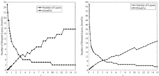
Furthermore, the algorithm performance to extract the multilayered thermal structure was evaluated using the abovementioned examples in terms of the number of layers detected as function of the preset convergence error ε and the final temperature retrieved error (%). In this case the al-gorithm was executed in a loop varyingεin the interval from 0.1 to 1.0 in steps of 0.1 and from 1.0 to 15 in a 0.5 step. The final temperature error was computed based on thenormof the final temperature vector resampled in terms of the origi-nal vector height. This explains why the actual preset value
ε, which applies to every step in the fitting and re-fitting pro-cess, is different from the final temperature profile error af-ter fitting the entire temperature profile. Figure 5 depicts two curves indicating the number of thermal layers retrieved and the final overall temperature error profile as a function of the
Figure 4.Analysis of radiosonde temperature profile: panel on the left represents temperature observation made on 15 January 2014 at 00:00 UTC and panel on the right is a GPS radiosonde observation during IOP WiBLEx on 13 October 2009 at 15:00 UTC both at the National Weather Service (NWS) Fairbanks International Station (code 70261). Vertical axis is height (m) above ground level.
Table 2.Results of application of the numerical routine to extract thermal layers from radiosonde database NOAA-ESRL PAFA 70261 for 15 January 2014 at 00:00 UTC and IOP WiBLEx GPS sounding on 13 October 2009 at 15:00 UTC. In this caseε=0.1 for both profiles. The temperature profile contains 32 points below 3 km height and the program detectedp=24 layers; for 13 October 2009 the sounding contains 677 points below 3 km andp=56 layers. In the classification column, the thermal inversion layers detected are indicated as SBI or EI. First column represents the layer number, second column is the layer base heightZb(m), third column is the layer top heightZt (m), fourth column is the temperature atZb, fifth column is the temperature atZt, sixth column is the temperature gradientmk(◦C/100 m), seventh column is the depth of the layer (m) and eighth column is the layer classification.
Layer Zb(m) Zt(m) Tb(◦C) Tt(◦C) mk(◦C/100 m) Depth (m) Classification
15 January 2014 00:00 UTC
2 62 165 −17.7 −12.3 5.2 165 SBI top 8 685 925 −8.7 −10.5 −0.7 240 EI 13 1108 1751 −7.9 −12.1 −0.6 643 EI
13 October 2009 15:00 UTC
5 35 44 0.4 0.7 3.5 44 SBI top 12 256 289 2.9 3.2 0.8 33.1 EI 15 371 425 3.8 4.3 0.7 53 EI 18 499 541 3.92 3.93 0.01 41.3 EI 20 615 654 3.8 4.3 1.0 39.2 EI 30 1069 1098 5.4 5.7 0.99 28.5 EI 32 1157 1213 5.5 5.7 0.35 56 EI 36 1484 1530 5.5 5.6 0.03 46 EI 41 1907 1983 4.1 4.3 0.23 76 EI 47 2346 2383 2.8 3.3 1.34 37 EI
In order to summarize the application of this methodol-ogy and visualize the effects of the final error over the recon-structed temperature profile, Fig. 6 illustrates the resampled temperature profile based on the case of four selected error levels for both cases.
It is clear that the lowest error (%) is associated with low-ering the convergence factorε, while on the other hand in-creasing the preset convergence factorεincreases the overall
Figure 5.Retrieved number of thermal layers (o) and final temperature profile error () as function of theεconvergence preset value. Panel on the left corresponds to 15 January 2014 at 00:00 UTC and panel on the right corresponds to 13 October 2009 at 15:00 UTC.
Figure 6. Resampled temperature profile after running the numerical methodology over different preset convergence factor valuesε=
0.1,1.0,5.5 and 10.5 as function of the final retrieved error (%). Panel on the left is for 15 January 2014 at 00:00 UTC and panel on the right is for 13 October 2009 at 15:00 UTC.
5 Summary
A simple numerical iterative routine was developed to de-duce thermal inversion layers composing a given atmo-spheric temperature profile. The numerical routine converts the temperature profile in a reduced data structure contain-ing base and top heights and temperatures as well as thermal gradients allowing identification of most important air mass changes accounting for surface-based inversion (SBI) and el-evated inversions (EI) present in the temperature sounding.
This methodology has been applied to the study of 10 years of upper air data in the interior of Alaska to deduce the statistical significance of the presence of SBI and multilevel EIs. In addition, the application of this methodology allowed classification of EI layers based on the type of synoptic air mass by means of the dew-point temperature gradient across the inversion layer depth (Mayfield and Fochesatto, 2013).
The method was also applied to study the temporal evo-lution of SBIs using high-resoevo-lution GPS soundings during the formation and breakup cycle in spring and fall seasons (Malingowski et al., 2014).
The method does not introduce new temperature points; it rather reduces the number of them according to the pre-set convergence factor. After the data structure is obtained, the determination of temperature inversion layers follows the search of changes in themkcoefficient.
classify them in terms of their dew-point temperature gradi-ent across the inversion depth. For that, it was necessary to include the dew-point temperature in the data structure after reading and processing the radiosonde data so that the re-trieved EI layer could be classified.
The relationship between threshold thermal gradient dT /dz, the preset convergence factorε and the overall fi-nal error between the resample temperature profile and the original temperature profile is not straightforward. Section 3 describes the relationship between dT /dzandεfor a theoret-ical profile to deduce this relationship. Section 4 applies the methodology, and then a resampled version of the tempera-ture profile was compared with the original temperatempera-ture pro-file to calculate an overall percent error. This is important to differentiate sinceεapplies internally as a convergence fac-tor to increase fidelity in the temperature fitting process over a Euclidean normthat applies over a variable vector length step by step. On the other hand, the overall error indicating how accurate the resampled temperature profile reproduces the original profile accounts for the entire profile at once.
The application of such methodology has numerous venues. For instance, air pollution meteorology and pollu-tant transport processes are strongly dependent on meteoro-logical conditions near the emission source – in particular at high latitudes where the SBI layers and stratified SBI show a persistent presence during the winter in the absence of or under a little diurnal cycle. The application of this method-ology is not restricted to low-level layers exclusively since it has been demonstrated by Mayfield and Fochesatto (2013) that EI layers also play an important role in the high-latitude ABL because of the dynamic–radiative forcing that drives surface warming and pollutant recirculation. Another appli-cation is the evaluation of large-scale synoptic meteorologi-cal changes and their impact on high-latitude environments. In this case it is important to consider a methodology that can scrutinize thermal layers present in the temperature profile over ocean, maritime and continental places. In order to be able to evaluate the impact of prescribed synoptic meteoro-logical patterns over a specific area, it is necessary to retrieve simultaneously thermal layers affected by local-scale and those dominated by large-scale atmospheric motion. There-fore evaluation of temporal series containing this multilay-ered information could assist in improving our understanding of how large-scale feedbacks are introduced and affect the lo-cal environment. Since the radiative interaction between SBI and EI layers is controlled by the vertical stratification, then the analysis of surface warming in high-latitude continental and oceanic environments in particular over sea-ice surfaces will be one future application of this methodology. Of course databases in which the method can be applied need to have sufficient vertical resolution to pull level details close to the surface to be able to define the multilayered structure.
The algorithm was proposed for radiosonde profiles, but it can also process temperature outputs from microwave ra-diometers and large-scale reanalysis databases as well as
cli-mate outputs downscaled to temperature profiles. Particularly interesting is the use of this algorithm in climatological de-termination of the temperature inversion layers SBI and EI and their connection to large-scale synoptic meteorology.
Acknowledgements. This research was funded by the Division of Air Quality from the Department of Environmental Conservation of Alaska and the Air Quality Office of the Fairbanks North Star Borough (funding number G00006433-398755). The author was supported by the Geophysical Institute, University of Alaska Fairbanks. The author acknowledge the use of the NOAA/ESRL reanalysis database. The author thanks Julie Malingowski for preparing and launching the high-resolution GPS soundings and the three anonymous reviewers for insightful comments that improved the article.
Edited by: G. Vulpiani
References
André, J. C. and Mahrt, L.: The nocturnal surface inversion and influence of clear-air radiative cooling, J. Atmos. Sci., 39, 864– 878, 1982.
Beyrich, F. and Weill, A.: Some Aspects of Determining the Sta-ble Boundary-Layer Depth from Sodar Data, Bound.-Lay. Mete-orol., 63, 97–116, 1993.
Bianco, L. and Wilczak, J.: Convective boundary layer depth: im-proved measurement by Doppler Radar wind profiler using fuzzy logic methods, J. Atmos. Ocean. Tech., 19, 1745–1758, 2002. Billelo, M. A.: Survey of arctic and subarctic temperature
inver-sions. US Army Cold Regions Research & Engineering Labora-tory, Hanover N. H., 36 pp., TR 161, 1966.
Bintanja, R., Graversen, R. G., and Hazeleger, W.: Arctic win-ter warming amplified by the thermal inversion and conse-quent los infrared cooling to space, Nat. Geosci., 4, 758–761, doi:10.1038/NGEO1285, 2011.
Bourne, S. M., Bhatt, U. S., Zhang, J., and Thoman, R.: Surface-based temperature inversions in Alaska from a climate perspec-tive, Atmos. Res., 95, 353–366, 2010.
Bowling, S. A., Ohtake, T., and Benson, C. S.: Winter pressure sys-tems and ice fog in Fairbanks, Alaska, J. Appl. Met., 7, 961–968, 1968.
Brooks, I. M.: Finding Boundary Layer Top: Application of a Wavelet Covariance Transform to Lidar Backscatter Profiles, J. Atmos. Ocean. Tech., 20, 1092–1105, 2003.
Byers, H. R. and Starr, V. P.: The circulation of the atmosphere in high latitudes during winter, Mon. Wea. Rev. Supplement No. 47, 34 pp., 1941.
Cassano, E. N., Cassano, J. J., and Nolan, M.: Synoptic weather pattern controls on temperature in Alaska, J. Geophys. Res., 116, D11108, doi:10.1029/2010JD015341, 2011.
Csanady, G. T.: Equilibrium theory of the planetary boundary layer with an inversion lid, Bound.-Lay. Meteorol., 6, 63–79, 1974. Curry, J. A.: On the formation of continental polar air, J. Atmos.
Sci., 40, 2279–2292, 1983.
Eastman, R. and Warren, S. G.: Interannual Variations of Arctic Cloud Types in Relation to Sea Ice, J. Climate, 23, 4216–4232, 2010.
Fochesatto, G. J., Drobinski, P., Flamant, C., Guédalia, D., Sarrat, C., Flamant, P. H., and Pelon, J.: Observational and Modeling of the Atmospheric Boundary Layer Nocturnal- Diurnal Transition during the ESQUIF Experiment, in: Advances in Laser Remote Sensing, edited by: Dabas, A., Loth, C., and Pelon, J., 439–442, Paris, France, 2001a.
Fochesatto, G. J., Drobinski, P., Flamant, C., Guedalia, D., Sarrat, C., Flamant, P., and Pelon, J.: Evidence of Dynamical coupling between the residual layer and the developing convective bound-ary layer, Bound.-Lay. Meteorol., 99, 451–464, 2001b.
Fochesatto, G. J., Ristori, P., Flamant, P. H., Ulke, A., Nicolini, M., and Quel, E.: Entrainment results in the case of strong mesoscale influences over the atmospheric boundary layer in the near coastal region, Peer reviewed contributions to the Interna-tional Laser Radar Conference, 231–234, Québec, Canada, 2002. Fochesatto, G. J., Ristori, P., Flamant, P. H., Machado, M., Singh, U., and Quel, E.: Backscatter LIDAR signal simulation applied to spacecraft LIDAR instrument design, Adv. Space Res., 34, 2227–2231, 2004.
Fochesatto, G. J., Collins, R. L., Yue, J., Cahill, C., and Sassen, K.: Compact Eye-Safe Backscatter Lidar for Aerosols Studies Urban Polar Environment, Proceedings of International Society for Optical Engineering, 5887, doi:10.1117/12.620970, 2005. Fochesatto, G. J., Collins, R. L., Cahill, C. F., Conner, J., and
Yue, J.: Downward Mixing in the Continental Arctic Boundary Layer during a Smoke Episode, Reviewed and revised papers presented at the Twenty-Third International Laser Radar Con-ference (ILRC), Nara, Japan, 24–28 July, 817–820, 2006. Fochesatto, G. J., Mayfield, J. A., Gruber, M. A.,
Starken-burg D., and Conner, J.: Occurrence of Shallow Cold Flows in the Winter Atmospheric Boundary Layer of Interior of Alaska, Meteorol. Atmos. Phys., Springer, Vienna, Austria, 1– 14, doi:10.1007/s00703-013-0274-4, 2013.
Garrat, J. R. and Brost, R. A.: Radiative cooling effect within and above the nocturnal boundary layer, J. Atmos. Sci., 38, 2730– 2745, 1981.
Hartmann, B. and Wendler, G.: Climatology of the winter surface temperature inversion in Fairbanks, Alaska, Proceedings of the 85th Annual Meeting of the American Meteorological Society, San Diego, CA, 1–7, 2005.
Holmgren, B., Spears, L., Wilson, C., and Benson, C.: Acoustic soundings of the Fairbanks temperature inversions, in: Climate of the Arctic, edited by: Weller, G. and Bowling, S. A., Proceed-ings of the AAAS-AMS conference, Fairbanks, Alaska, 293– 306, 1975.
Huff, D. M., Joyce, P. L., Fochesatto, G. J., and Simpson, W. R.: Deposition of dinitrogen pentoxide,N2O5, to the snowpack at high latitudes, Atmos. Chem. Phys. Discuss., 10, 25329–25354, doi:10.5194/acpd-10-25329-2010, 2010.
Kahl, J.: Characteristics of the low-level temperature inversion along the Alaskan Arctic coast, Int. J. Clim., 10, 537–548, 1990. Kahl, J. D., Serreze, M. C., and Schnell, R. C.: Tropospheric low-level temperature inversions in the Canadian Arctic, Atmos.-Ocean, 30, 511–529, 1992.
Lammert, A. and Bosenberg, J.: Determination of the convective boundary-layer height with Laser Remote Sensing, Bound.-Lay. Meteorol., 119, 159–170, 2006.
Mahrt, L., Vickers, D., Nakamura, R., Sun, J., Burns, S., and Lenschow, D.: Shallow drainage flows, Bound.-Lay. Meteorol., 101, 243–260, 2001.
Malingowski, J., Atkinson, D., Fochesatto, G. J., Cherry, J., and Stevens, E.: An Observational Study of Radiation Temperature Inversions in Fairbanks, Alaska, Polar Science, 8, 24–39, 2014. Mayfield, J. A. and Fochesatto, G. J.: The Layered Structure of the
winter Atmospheric Boundary Layer in the Interior of Alaska, J. Appl. Meteorol. Clim., 52, 953–973, 2013.
Menut, L., Flamant, C., Pelon, J., and Flamant, P. H.: Urban boundary-layer height determination from lidar measurements over the Paris area, Appl. Opt., 36, 945–954, 1999.
Milionis, A. E. and Davies, T. D.: A five-year climatology of ele-vated inversions at Hemsby (UK), Int. J. Climatol., 12, 205–215, 1992.
Milionis, A. E. and Davies, T. D.: The effect of the prevailing weather on the statistics of atmospheric temperature inversions, Int. J. Climatol., 28, 1385–1397, 2008.
Overland, J. E. and Guest, P. S.: The Arctic snow and air temper-ature budget over sea ice during winter, J. Geophys. Res., 96, 4651–4662, 1991.
Raddatz, R. L., Galley, R. J., Candlish, L. M., Asplin, M. G., and Barber, D. G.: Integral Profile Estimates of Sensible Heat Flux from an Unconsolidated Sea-Ice Surface, Atmos.-Ocean, 51, 135–144, doi:10.1080/07055900.2012.759900, 2013a. Raddatz, R. L., Galley, R. J., Candlish, L. M., Asplin, M. G., and
Barber, D. G.: Integral Profile Estimates of Latent Heat Flux under Clear Skies at an Unconsolidated Sea-Ice Surface, Atmos.-Ocean, 51, 239–248, doi:10.1080/07055900.2013.785383, 2013b.
Robbins, C. C. and Cortinas, J. V.: Local and synoptic environments associated with freezing rain in the contiguous United States, Weather Forecast., 17, 47–65, 2002.
Seidel, D. J., Ao, C. O., and Li, K.: Estimating climatological plane-tary boundary layer heights from radiosonde observations: Com-parison of methods and uncertainty analysis, J. Geophys. Res., 115, D16113, doi:10.1029/2009JD013680, 2010.
Serreze, M. C., Kahl, J. D., and Schnell, R. C.: Low-level tempera-ture inversions of the Eurasian Arctic and comparisons with So-viet drifting station data, J. Climate, 5, 615–629, 1992.
Shulski, M. and Wendler, G.: The Climate of Alaska, University of Alaska, Fairbanks, 216 pp., 2007.
Whiteman, C. and Zhong, S.: Downslope Flows on a Low-Angle Slope and Their Interactions with Valley Inversions, J. Appl. Me-teorol., 47, 2023–2038, 2008.
Zhang, Y. and Seidel, D. J.: Challenges in estimating trends in Arc-tic surface-based inversions from radiosonde data, Geophys. Res. Lett., 38, L17806, doi:10.1029/2011GL048728, 2011.