Compound extremes in a changing climate – a Markov chain approach

www.nonlin-processes-geophys.net/23/375/2016/ doi:10.5194/npg-23-375-2016

© Author(s) 2016. CC Attribution 3.0 License.

Compound extremes in a changing climate –

a Markov chain approach

Katrin Sedlmeier1,a, Sebastian Mieruch1,b, Gerd Schädler1, and Christoph Kottmeier1

1_{Institute for Meteorology and Climate Research, Karlsruhe Institute of Technology, Karlsruhe, Germany} a_{now at: Federal Office of Meteorology and Climatology MeteoSwiss, Zurich, Switzerland}

b_{now at: Alfred-Wegener-Institut, Helmholtz-Zentrum für Polar- und Meeresforschung, Bremerhaven, Germany} Correspondence to:Katrin Sedlmeier (katrin.sedlmeier@meteoswiss.ch)

Received: 1 December 2015 – Published in Nonlin. Processes Geophys. Discuss.: 19 February 2016 Revised: 10 September 2016 – Accepted: 13 September 2016 – Published: 1 November 2016

Abstract.Studies using climate models and observed trends indicate that extreme weather has changed and may con-tinue to change in the future. The potential impact of extreme events such as heat waves or droughts depends not only on their number of occurrences but also on “how these extremes occur”, i.e., the interplay and succession of the events. These quantities are quite unexplored, for past changes as well as for future changes and call for sophisticated methods of anal-ysis. To address this issue, we use Markov chains for the analysis of the dynamics and succession of multivariate or compound extreme events. We apply the method to observa-tional data (1951–2010) and an ensemble of regional climate simulations for central Europe (1971–2000, 2021–2050) for two types of compound extremes, heavy precipitation and cold in winter and hot and dry days in summer. We identify three regions in Europe, which turned out to be likely sus-ceptible to a future change in the succession of heavy precip-itation and cold in winter, including a region in southwestern France, northern Germany and in Russia around Moscow. A change in the succession of hot and dry days in summer can be expected for regions in Spain and Bulgaria. The suscep-tibility to a dynamic change of hot and dry extremes in the Russian region will probably decrease.

1 Introduction

Multivariate extreme events (in this paper used in the sense of extremes of two or more climate variables occurring si-multaneously) are likely to impact society greater than their

univariate counterparts. For agriculture for example, the im-pact of a heat wave and a drought occurring at the same time is higher than for a univariate extreme where the other vari-able is in a normal state. These multivariate or so-called com-pound events (IPCC, 2012) have received more and more attention in the scientific literature over the past years al-though still not to the extent of extremes of only one vari-able. Methods to analyze them include simple threshold analysis, multivariate distribution functions using copulas (e.g., Schölzel and Friederichs, 2008; Durante and Salvadori, 2010), Bayesian approaches (e.g., Tebaldi and Sansó, 2009) or indices that are derived from multiple variables (e.g., the wildfire index KBDI, e.g., Keetch and Byram, 1968, or the revised CEI, Gallant et al., 2014). Furthermore, methods of multivariate extreme models have been used for the geo-statistical analysis of spatially distributed extremes (Neves, 2015). All these methods focus mostly on the linear climate change signal – the absolute change in the number of oc-currences or the calculation of return periods. The succes-sion, i.e., the temporal ordering of the compound events, is in most cases not the main objective. For instance, the IPCC (IPCC, 2012) states: “A changing climate leads to changes in the frequency, intensity, spatial extent, duration, and tim-ing of extreme weather and climate events, and can result in unprecedented extreme weather and climate events”. What is implicitly addressed with “duration and timing”, but not ex-plicitly stated is the succession of extreme events, which is quite unknown for past as well as future extremes.

of climate change, which has not received much attention up to now, but is nevertheless important. We investigate a be-havior of extremes, which cannot be determined by simply analyzing the changes in the number of extremes. We can, for example, reveal changes in the entropy of the succession of compound extremes, which are connected to the chaotic behavior of the climate variable. Thus, an observed increase of this measure could be connected with an increase in the chaotic, intermittent or irregular nature of the system. On the other hand, a decrease of entropy corresponds to a slowdown of these dynamics. Knowledge about such developments for future climate, which rarely exists, could be important for many sectors, e.g., agriculture, economy and society.

Previous studies on model dynamics have concentrated more on overall dynamical behavior, such as (Steinhaeuser and Tsonis, 2014), who conducted a model intercomparison study focusing on dynamical aspects based on a climate net-works framework. The method introduced in this paper is inspired by the work of (Mieruch et al., 2010). The idea is to understand climate time series as trajectories on a com-plex, possibly strange attractor (Lorenz, 1963). We partition the time series or state space into a finite number of states. This yields a coarse-grained description of the system, which can then be analyzed in the framework of symbolic dynam-ics (Ebeling et al., 1998; Daw et al., 2003). We apply a Markov chain analysis on these symbolic sequences repre-senting compound extremes, and characterize their dynami-cal or successional behavior using a small set of descriptors. In this paper we study two different kinds of compound extreme events that are likely to have an impact on society, namely, cold and heavy precipitation in winter, and heat and drought in summer. The Markov method is applied to E-OBS observational data (1951–2010) (Haylock et al., 2008), and an ensemble of regional climate simulations with the regional climate model COSMO-CLM (COnsortium for Small scale MOdelling model – in CLimate Mode) driven by different global climate model data and ERA-40 reanalysis (Uppala et al., 2005). The time periods considered are the recent past (1971–2000) and the near future (2021–2050).

We identify regions in Europe, where the dynamical be-havior of the analyzed compound extremes is prone to change. These findings highlight that it is not only the (sim-ple) linear increase of the occurrence of extremes (due to an increase in mean and variability), which is a challenge for adaption and mitigation. In addition to these changes, the re-gions also have to struggle with changes in the succession of compound extremes (defined as relative to a new normal state with changed mean and variability).

The strategy of this study is first to show that the Markov method is able to extract different dynamics of compound extremes for different regions in Europe, based on observa-tional data and model data. Thus, on the one hand we see that the method yields meaningful information and on the other hand we show that the climate models are able to reproduce these dynamics in the frame of acceptable uncertainties.

Ad-ditionally, we extract temporal change signals of the dynam-ics of compound extremes based on observations between the periods 1951–1980 and 1981–2010. This information is new and if used as supplementary information to other analyses, could lead to a better understanding of changes of extremes in Europe. For this paper, the magnitude of the observed past changes have been assessed, because it is important for a bet-ter inbet-terpretation and classification of future changes, which are calculated by using the simulated regional climate model data. A comparison of the change signals between 1971– 2000 and 2021–2050 to the observed past changes shows that they are of the same order of magnitude.

The paper is divided into the following sections. In Sect. 2, data and method will be introduced, followed by a sensitiv-ity analysis of the method with respect to spatial and tem-poral variability as well as the error of estimation using FT (Fourier transform) surrogates in Sect. 3. A validation of the model ensemble is shown in Sect. 4. The change signal is analyzed in Sect. 5. A summary and outlook will be given in Sect. 6 and some areas discussed where the application of this method might be of value.

2 Data and methods

2.1 Regional climate ensemble

all weighed with a factor of one-fifth when calculating the mean. All other models receive a factor of 1, which leads to an effective ensemble size of eight. Additionally we use a COSMO-CLM run driven by ERA-40 (Uppala et al., 2005) boundary conditions. The ERA-40 reanalysis boundary con-ditions are assumed to be close to the “true” observed state. Nevertheless, they depend on, inter alia, the model, obser-vational data and assimilation technique, and are not free from biases (see e.g., Hagemann et al., 2005; Simmons et al., 2004).

The simulation time periods are the recent past (1971– 2000) and the near future (2021–2050). An analysis of the temperature trends of different ensemble members showed that the distribution of trend depends more strongly on the chosen global climate model than on the emission scenario. We therefore combine simulations with boundary data from GCMs with different emission scenarios to set up our ensem-ble.

We choose six regions, each comprising 6×6 grid points for our analysis. The regions are chosen based on the PRU-DENCE regions (Christensen and Christensen, 2007), which could not be used because of the necessity of the same amount of grid points for each area, and due to test results that show a different behavior for these regions. We inves-tigate 30-year periods of daily data; thus, each time series consists of _≈11 000 data points, yielding_≈36_×11 000_≈ 400 000 points in time for each region and ensemble mem-ber. The model domain and the six investigation areas, which are located in Spain, France, Germany, Scandinavia, Bulgaria and Russia, are shown in Fig. 1. These roughly match the PRUDENCE regions, which are not applicable for the analy-sis since equal sized areas are a requirement for comparison among regions.

2.2 Observational data

For the comparison of our regional climate ensemble with observations, we use temperature and precipitation data from the gridded E-OBS data set (Haylock et al., 2008). This data set was produced as part of the ENSEMBLES project by interpolating station data from the ECA&D station data set (European Climate Assessment; Klok and Klein Tank, 2009) to a 25 km grid. The station density is highest in Switzer-land, the Netherlands and Ireland and rather low in Spain and the Balkans, which leads to an over-smoothing in these areas. This especially affects extremes and has to be taken into account when validating our ensemble against E-OBS data. Furthermore it should be noted that a comparison of E-OBS and another gridded data set, namely, Hyras (Rauthe et al., 2013) (only central Europe), with respect to the dynam-ical behavior that we analyze in this paper, revealed differ-ences between the two data sets (Sedlmeier, 2015). A com-parison of dynamical aspects of different observational data sets yields an interesting application of the method, which, however, will not be addressed within this paper. We

addi-Figure 1.E-OBS descriptors for the reference period (1971–2000). Left side: descriptors for cold and wet extremes in winter (DJF)

(Ta<10th percentile and Pa>75th percentile). Right side:

descrip-tors for hot and dry extremes in summer (JJA) (Ta>90th

per-centile and EDI<25th percentile). Descriptors were calculated for

a moving window over nine grid points and values assigned to the center grid point (see text). Boxes show the PRUDENCE regions (http://ensemblesrt3.dmi.dk/quicklook/regions.html).

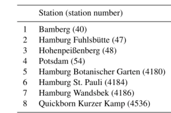
Table 1.ECA&D station data.

Station (station number)

1 Bamberg (40)

2 Hamburg Fuhlsbütte (47)

3 Hohenpeißenberg (48)

4 Potsdam (54)

5 Hamburg Botanischer Garten (4180)

6 Hamburg St. Pauli (4184)

7 Hamburg Wandsbek (4186)

8 Quickborn Kurzer Kamp (4536)

tionally use blended temperature and precipitation time se-ries starting from 1900 of eight stations (all in Germany) of the ECA&D data set for a sensitivity analysis described in Sect. 3. The eight stations are listed in Table 1.

2.3 Compound extremes with Markov chain descriptors

sub-tidal community. It has been introduced to atmospheric sci-ence by (Mieruch et al., 2010), who used it for climate clas-sification and a comparative study of two regions. In this sec-tion, a short introduction to Markov chains is given, followed by a step by step description of the method.

A first-order,mstate (mis the number of discrete states of the Markov chain), homogeneous Markov chain is a time discrete, state discrete stochastic process, which fulfills the Markov property:

P (xt|xt₋1, xt₋2, . . ., xt₋n)=P (xt|xt₋1) , (1) meaning that the present state xt is only dependent on the preceding state xt₋1. From the Markov chain, a transi-tion probability matrix Pof the orderm_×mcan be calcu-lated, which consists of all possible conditional probabili-tiesP (xt|xt−1)between themdifferent states of the Markov chain. For a homogeneous (≡stationary) Markov chain, the transition probability matrix is time independent. A station-ary distributionπis a vector that fulfills the following equa-tion

π=Pπ. (2)

To test for homogeneity one must solve the eigenvalue prob-lem of Eq. (2) to calculate the stationary distribution π. If this is identical to the empirical distribution

ˆ

πj =

nj

P

jnj

(3) the time series is considered stationary. The entries (transi-tion probabilities) of the transi(transi-tion matrixPare estimated by

ˆ

pij=

nij

P

inij

. (4)

In the following, the main steps of the Markov analysis are explained:

a. Partitioning and combining of univariate time series to a multivariate symbolic sequence

To represent the univariate time series (here daily mean temperature anomalies and daily precipitation anoma-lies) by a Markov chain, each time series is partitioned into a symbolic sequence of extreme and non-extreme regimes. These univariate symbolic sequences are then combined into a multivariate symbolic sequence ofm₌

2v_{different states (vnumber of variables). In this paper,}

v₌2; thus, there are four possible states. b. Calculation of the transition probability matrix

From the 2v-state Markov chain, a transition probability matrixPof dimension 2v×2vcan be calculated. Two conditions have to be met when calculating the descrip-tors. No entry of the transition probability matrix should be equal to zero and the time series needs to be station-ary for the transition probability matrix to be time inde-pendent (see Eqs. 2, 3).

c. Calculation of the descriptors

Following Mieruch et al. (2010), we focus on only three of the descriptors mentioned in Hill et al. (2004): per-sistence, recurrence time and entropy. These descriptors can be estimated for single states of the symbolic se-quence or for the whole system. As the focus of this work lies on the compound extreme state, only the single-state definition of the descriptors is considered.

- Persistence:

Pj= ˆpjj. (5) The persistence gives the probability that the sys-tem will stay in an extreme state in the following time step if it resides in an extreme state at the cur-rent time step. The limits are 0 (the system will never stay in the extreme state) and 1 (the system will always stay in the extreme state). Regarding the succession of the compound extremes, the per-sistence tells us how long the extremes last. - Recurrence time:

Rj=

1_{− ˆ}πj 1_{− ˆ}pjjπˆj

. (6)

The recurrence time describes the number of days the system needs to get back to the extreme state. The limits are 0 (the system never leaves the state, corresponding to a persistence of 1) and_∞(the sys-tem never comes back to the extreme state). The re-currence time is connected to the persistence. If the persistence increases, the recurrence time will also increase and vice versa, except if a change in the number of statesπ_ˆj occurs. Thus, it is important to include the absolute number of the states for the interpretation of the results.

- Entropy:

H pj

= −X

i ˆ

pijlogpˆij/log

1

m

. (7)

attractors, are more suitable. Thus, in the sense of successive compound extremes a change in entropy tells us if the succession of extreme states gets more chaotic or more regular.

d. Data pre-processing

In order to extract the information on successive com-pound extremes, we have to remove linearities (e.g., trends) and cycles, which would bias the results. Thus, we remove the external solar forcing by subtracting the mean annual cycle. A long-term trend is removed by a linear regression. Although, e.g., the temperature trend due to the anthropogenic CO2 emissions is removed from the data, we hypothesize that all changes in the succession of extremes are linked to the CO2increase. The reason for this is that the CO2forcing is the only difference between the model runs for the periods 1971– 2001 and 2021–2050.

We use percentiles to partition our data sets, and keep the number of univariate extreme events the same for different time periods and regions as well as for all en-semble members. By this, the results can be compared among each other, differences are only due to different dynamical behavior. For partitioning dry days, we did not use precipitation anomalies but the effective drought index (EDI). The EDI (see Sect. 2.4) is related to soil moisture and is therefore a much better measure for de-scribing dry extremes than precipitation itself, since all percentiles below the percentage of dry days will lead to the same partitions.

In order to get a better feeling for the descriptors and un-derstand how they relate with each other, we will do a small thought experiment. We take a Markov chain consisting of a time series of 1000 symbols of which 10 % are extreme, the rest are normal. In this case a persistence of 0.5 would mean that in half of the 100 extreme cases, the next case is also extreme, there are 50 transitions from the extreme state to the extreme state. The maximum episode length in this case is thus 51 extreme states in a row (with all others randomly distributed). The recurrence time and entropy are inversely related to how these 50 extreme transitions are ordered. Re-currence time depends on the number of episodes (fewer episodes lead to a larger recurrence time, more episodes to a shorter recurrence time) and entropy additionally on the mean episode length. In this paper, we also look at changes in the descriptors. A change in persistence of 0.05 in the above case would mean five more extreme–extreme transi-tions per 1000 days, and an increase from 50/100 to 55/100 (extreme–extreme transitions/extreme–normal transitions) is surely a noticeable change. The range of actually probable values of the descriptors is smaller than the whole possible range. A persistence of 0.99 for example, would mean that there is only one extreme episode in the whole time period, all 100 extreme states occur after each other. In a climate

system, this is unlikely to happen. Thus, for climate one can-not expect to observe a change of the daily persistence from, e.g., 0.5 to 0.8, because such a change would be catastrophic. 2.4 Effective drought index: EDI

The EDI is an index for detecting drought conditions by cal-culating daily deviations of precipitation from a climatologi-cal mean state. It was proposed by Byun and Wilhite (1999). An important concept of the EDI is the use of effective pre-cipitation (EP), rather than prepre-cipitation (P) itself. EP de-scribes the depletion of water sources by a weighted summa-tion over the 365 days preceding a given day (d):

EPd₌ 365

X

n=1

Pn

m=1Pd₋m

n

. (8)

By this, the memory effect of the soil is taken into account. Therefore, EP strongly correlates with soil moisture and the EDI is thus a good measure when considering droughts. Us-ing the EP, the EDI is calculated by the followUs-ing formula for a givend:

EDId=

EPd₋EPd,rm

σ EP₋EP

d

, (9)

where EPd,rm is the climatological mean corresponding to a given d calculated as the 30-year average over a 5-day-running mean (rm₌5). By subtracting this climatological mean of EP from the daily value, the yearly cycle is removed from the EDI time series.

2.5 The Markov descriptors for two compound extremes

To calculated the Markov descriptors, we first calculated temperature and precipitation anomalies using the mean an-nual cycle of the respective time period and ensemble mem-ber/observation. We calculate the Markovian descriptors for two types of extremes:

– cold and heavy precipitation (temperature anomaly (T)<10th percentile and precipitation anomaly (P)>75th percentile) in winter (DJF)

– heat and drought (P >90th percentile and EDI<25th percentile) in summer (JJA)

S_h,h,t and then a Markov chain could look likeS_l,h,1,S_l,l,2,

S_l,l,3,S_h,h,4,S_h,h,5,S_h,h,6,S_h,l,7, . . ., S_h,h,N, whereN is the total number of data points. From such a sequence we cal-culate the transition probability matrix and from this, the de-scriptors.

3 Sensitivity analysis

Before applying the method to the observational data and the model ensemble, we tested the applicability of the method by several sensitivity tests using the above-defined descriptors. Therefore, we consider the gridded E-OBS data and addi-tionally ECA&D station data.

3.1 Spatial variability

In order to test the spatial variability of the descriptors, we calculated them for the entire E-OBS data set for the time period 1971–2000 for the two types of extremes mentioned above.

The descriptors were calculated for each grid point, taking into account not only this grid point but also the eight neigh-boring grid points thus using a moving window if nine grid points. The time series for each grid point were detrended and partitioned separately before the nine partitioned time series were merged to calculate the descriptors. The reason for using this moving window of nine grid points is the ful-fillment of the criteria of the Markov method (see Sect. 2.3), which is not given for the entire area when using only sin-gle grid points. Using this moving window does not alter the general spatial pattern and smoothness of the results.

For both type of extremes, the descriptors show smooth spatial patterns (see Fig. 2); nevertheless, variations between different regions can be identified.

The persistence for the winter extremes (left side of Fig. 2) is lower than for summer extremes; specifically, in northern and central Europe compound cold and wet events are most likely events of a short duration and rather rare (with recur-rence times of up to 400 days). Along the Mediterranean coast and southeastern Europe, the values are higher and probabilities of residing in a compound extreme state of over 50 % are observed. The recurrence time for these events is also comparatively low (around 100 days). Interpreting the results, one has to keep in mind that we are always referring to relative compound extremes. The entropy is around 0.9 for most of the area with small regions showing lower entropies down to 0.5. These high values can be explained by the low persistence – as compound winter extremes are grouped in very short episodes (low persistence), they are very hard to predict. The highest persistence for summer events (right side of Fig. 2) are observed in Scandinavia and the eastern part of the E-OBS domain and lowest in central Europe and the northern coast of Spain. The persistence is above 50 % for the whole domain, which means that the probability of the

Figure 2.Elevation of the CCLM 50 km model domain [m]. Boxes mark the six investigation areas – 1: Spain (black), 2: France (red), 3: Germany (green), 4: Scandinavia (blue), 5: Russia (cyan) and 6: Bulgaria (magenta).

system residing in a compound extreme state is high and these events are grouped in episodes of long duration. The recurrence time lies between 40 and 100 days and is as such also lower than that for compound winter events. The lowest values are observed in the Balkan region. The entropy lies between 0.4 and 0.65, which means that the extreme events are not so easy to predict, especially for parts of central Eu-rope where the entropy is the highest. However, according to our definitions, summer extremes can better be predicted than winter extremes.

re-gions, we chose regions consisting of 6_×6 grid points from within these widely used regions. The regions that will be analyzed in the further sections of this paper are shown in Fig. 1.

Note that the results shown in Fig. 2 can only be qualita-tively compared to those of the regions considered later or the station data in the next section as the number of grid points (or stations) contributing to the analysis differs.

3.2 Temporal variability

To assess the temporal variability of the descriptors, we cal-culated the descriptors for 30-year moving windows of ob-servational station data from the ECA&D station data set (Klein Tank et al., 2002). Since we are interested in the daily values of temperature and precipitation, only stations were chosen with a continuous daily record (with an allowance of 50 missing values at most). Using these criteria there are eight stations with temperature and precipitation time series from 1900 to 2015 of which all are in Germany (see Table 1). One station has 15 missing values for temperature. These days were excluded from the analysis, considering the 30-year time windows consisting of 10 950 days, this amounts to roughly 0.1 % of the values and does not alter the value of the descriptors. Of these eight stations, five are in the vicin-ity of Hamburg and have the same values for the first 17– 22 years. The records of two stations in Hamburg are identi-cal throughout the whole time period; therefore, only one of them is included in the analysis, which leaves a total of seven stations.

The descriptors were again calculated for both types of compound events. Linear temperature trends were removed separately for each of the 30-year time windows and in or-der to fulfill the criteria of the Markov method (stationarity and non-zero entries of the transition probability matrix; see Sect. 2.3), the partitioned data of these seven stations were combined to one time series to calculate the descriptors.

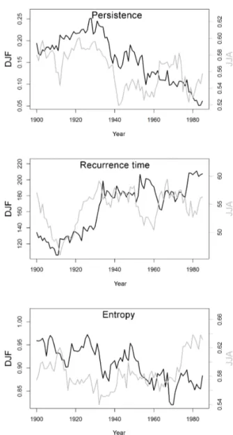
The results are shown in Fig. 3 for both winter (black) and summer (gray) extremes. Especially for the persistence and recurrence time, a clear shift is visible between 1930 and 1950. This time range is not preindustrial, but the cru-cial point is that the observed shift coincides with an ob-served shift in the global increase in CO2around 1950 (see, e.g., IPCC, 2014, Fig. SPM.1d). From this finding we ob-serve two main points:

1. The descriptors (especially persistence and recurrence time) seem to be sensitive to changes of the CO2 increase. That means a stronger increase of CO2 (e.g., from 1950 on) yields a lower level of persis-tence and to a higher level of recurrence time. Al-though CO2is still increasing after 1950, the recurrence time, e.g., remains constant. Hence, the recurrence time seems not to be dependent on the absolute CO2 concen-tration, but on the increase of latter.

Figure 3.Descriptors for ECA&D station data for running windows over 30 years (values are assigned to the first year of the 30-year time period) from 1900 to 2015. Black curve: cold and wet extremes

in winter (DJF) (Ta<10th percentile and Pa>75th percentile).

Gray lines: hot and dry extremes in summer (JJA) (Ta>90th

per-centile and EDI<25th percentile).

2. Thus, we can conclude that the natural variability of the descriptors can be approximated by the variability ob-served before and after the shift. This natural variability is smaller than the shift of the mean.

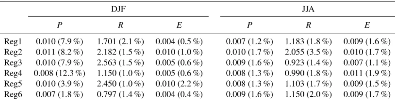
Table 2.Estimation of the error of the descriptors by using MIAAFT surrogates for winter and summer extremes. The values were calculated using the E-OBS data set for the reference period (1971–2000). In parentheses the percentage of the error with respect to the value of the E-OBS descriptors for the same time period and region are given.

DJF JJA

P R E P R E

Reg1 0.010 (7.9 %) 1.701 (2.1 %) 0.004 (0.5 %) 0.007 (1.2 %) 1.183 (1.8 %) 0.009 (1.6 %)

Reg2 0.011 (8.2 %) 2.182 (1.5 %) 0.010 (1.0 %) 0.010 (1.7 %) 2.055 (3.5 %) 0.010 (1.7 %)

Reg3 0.010 (7.9 %) 2.563 (1.5 %) 0.005 (0.6 %) 0.009 (1.6 %) 0.923 (1.4 %) 0.007 (1.1 %)

Reg4 0.008 (12.3 %) 1.150 (1.0 %) 0.005 (0.6 %) 0.008 (1.3 %) 0.990 (1.8 %) 0.011 (1.9 %)

Reg5 0.010 (3.9 %) 2.450 (1.0 %) 0.010 (2.2 %) 0.008 (1.3 %) 1.103 (1.7 %) 0.009 (1.5 %)

Reg6 0.007 (1.8 %) 0.797 (1.4 %) 0.004 (0.4 %) 0.009 (1.6 %) 1.150 (2.0 %) 0.009 (1.7 %)

P: persistence,R: recurrence time,E: entropy.

changes of the descriptors (1971–2000 vs. 2021–2050) pre-sented below (see Sect. 6), we find changes of the persistence larger than 50 % and changes of the recurrence time larger than 20 %. We additionally perform significance tests on our results, which show that these changes are indeed significant, excluding natural variability as the source for the observed changes.

3.3 Error of estimation using Fourier transform (FT) surrogates

To assess the estimation error of the descriptors we used the Multivariate Iterated Amplitude Adjusted Fourier Transform (MIAAFT) algorithm as described by Venema et al. (2006) and Schreiber and Schmitz (2000). With this algorithm, the data are shuffled and thus the original distribution is pre-served. In addition, the auto- and cross-correlation of the temperature and precipitation time series are approximately preserved. We constructed 100 MIAAFT surrogates for the temperature and precipitation anomalies (or the EDI time se-ries for summer events, respectively) for the E-OBS data set for the reference period (1971–2000). We then estimated the standard deviation of the descriptors calculated from these surrogate time series. It is important to note that this stan-dard deviation, under the framework of such a bootstrap test, already represents the standard error of the mean, which cor-responds to the normal standard deviation divided by √N. The errors for both types of extremes and the six regions are listed in Table 2. The errors do not vary much between the different extremes and regions, the error of the persistence is on the order of 0.01 or lower, for the recurrence time be-tween 1 and 2.6 and the error of the entropy on the order of 0.005. Adopting these errors to the values of the E-OBS de-scriptors for the reference period (shown in Figs. 4 and 5 in Sect. 4), the error of the persistence is about 2–10 %, for the recurrence time about 2 % and for the entropy about 1–2 % (cf. Table 2).

This estimation error is much smaller than the ensemble uncertainty and can approximately be neglected. This shows

that the estimation of the descriptors is robust. Further, we will consider the E-OBS data approximately as truth and we will use the ensemble uncertainty as the error for our main analysis.

4 Markovian descriptors for the reference period 1971–2000

Figure 4.Descriptors for cold and wet extremes in winter (DJF) (Ta<10th percentile and Pa>75th percentile) in the reference period 1971– 2000 for the six investigation areas. Box plots of the CCLM ensemble: box is the ensemble median and interquartile range and whiskers are ensemble minimum/maximum; gray bars: ensemble mean; triangles: reanalysis-driven CCLM runs; crosses: E-OBS observations. The coloring corresponds to the regions in Fig. 1.

Figure 5.Descriptors for hot and dry extremes in summer (JJA) (Ta>90th percentile and EDI<25th percentile) in the reference period 1971–2000 for the six investigation areas. Box plots of the CCLM ensemble: box is the ensemble median and interquartile range and whiskers are ensemble minimum/maximum; gray bars: ensemble mean; triangles: reanalysis-driven CCLM runs; crosses: E-OBS observations. The coloring corresponds to the regions in Fig. 1.

Focusing on the descriptors for the CCLM ensemble (box plots and gray bars in Fig. 4), we can see that with this method we are able to detect significant differences in dy-namical behavior between some of the regions. In compari-son to the descriptors of the observations (crosses in Fig. 4), the ensemble is able to capture the differences between the regions fairly well except for the persistence in region 5, where the ensemble shows a much lower persistence and the recurrence time of region 4 (Scandinavia), which is lower for the observations. However, these are regions where the den-sity of station data underlying the E-OBS data set is not very high and the E-OBS results may not be as reliable. The high-est persistence is again in region 6 (Bulgaria), which also shows the lowest recurrence time and therefore has compar-atively long events that occur more frequently than in other areas. The triangles mark the descriptors of the reanalysis-driven simulations. They fit well for some regions, for others they are farther away from the observations than the CCLM-ensemble.

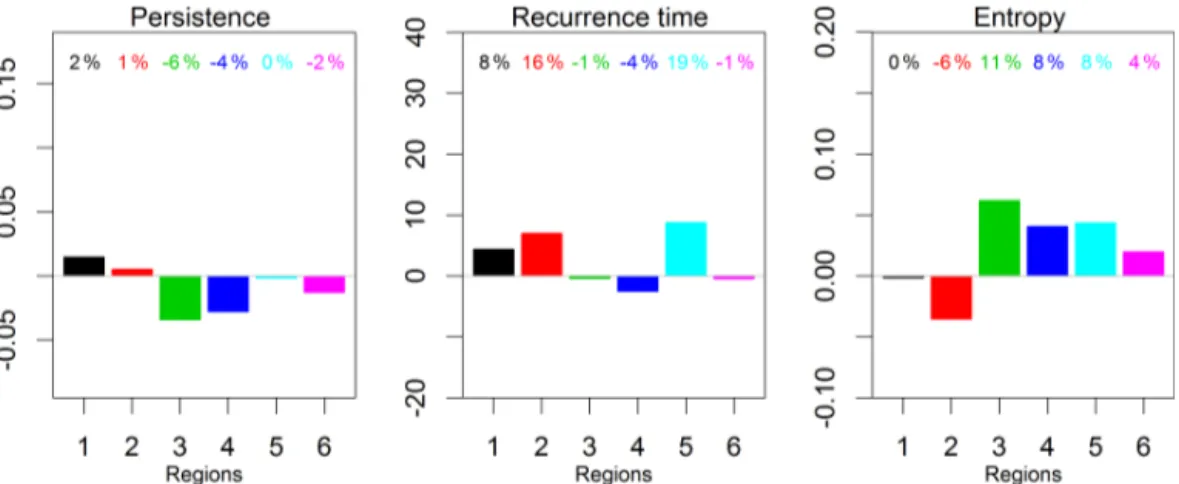
Figure 6.Change signal of descriptors for E-OBS observations: cold and wet extremes in winter (DJF) (Ta<10th percentile and Pa>75th percentile). Changes between the time periods 1951–1980 and 1981–2010. Percentages denote the relative change. The coloring corresponds to the regions in Fig. 1.

by the total number of extremes). The CCLM ensemble (box plots) again captures the tendencies of the observed descrip-tors fairly well but shows a large spread and differences be-tween the regions are mostly not significant for persistence and recurrence time. The ERA-40-driven CCLM simulations (triangles in Fig. 5) again fit well to the observations for some regions and show very different behavior for others.

For both types of compound extremes the ensemble mean and median seem to be able to capture the differences be-tween regions shown by observations although not always in absolute numbers. An interesting result is that reanalysis-driven CCLM data are sometimes farther away from the ob-servational descriptors than the model data, especially for the cold and wet extremes in winter. This leads to the ques-tion whether the dynamical behavior of the driving GCM is greatly altered by the RCM downscaling or errors in both models compensate during the downscaling process. A fur-ther cause of this deviation of the ERA-40-driven simula-tions could be a misrepresentation of the dynamics by the reanalysis data set. A follow up study comparing dynamical behavior of both RCM and GCMs is planned for the future. Additionally, it would be interesting to also compare differ-ent reanalysis data sets using this method as there have been studies showing differences in their variability (e.g., Hage-mann et al., 2005).

5 Climate change signal of the Markovian descriptors 5.1 Change signal within the reference period

In order to get an idea about the order of magnitude of the change signal, the observational E-OBS data set was split into two equal parts of 30 years, 1951–1980 and 1981–2010. The descriptors were calculated for both time periods and a change signal derived.

For cold and wet extremes (see Fig. 6) all regions ex-cept France show a decrease in persistence, regions 5 and 6 (Russia and Balkan) show the strongest absolute decrease (_≈0.15) and Germany the highest relative decrease of₋72 % (relative changes are shown above the respective bars). The recurrence time does not change much for all regions except region 5 (Russia) where it decreases by 150 days. In this re-gion, compound cold and wet extremes occurred more fre-quently but were of shorter duration in 1981–2010. The en-tropy shows a decrease of more than 5 % in Spain and Ger-many where the system becomes more regular. In Spain an increase of entropy is observed and the compound extremes are harder to predict in 1981–2010 with respect to 1951– 1980. The change signal for all descriptors and seasons (ex-cept for the entropy of France and Russia) are greater than the estimated error by FT-surrogates (see Table 2); thus, these changes are robust.

Figure 7.Change signal of descriptors for E-OBS observations: hot and dry extremes in summer (JJA) (Ta>90th percentile and EDI<25th percentile). Changes between the time periods 1951–1980 and 1981–2010. Percentages denote the relative change. The coloring corresponds to the regions in Fig. 1.

Figure 8.Number of compound cold and wet extremes in winter

(DJF) (Ta<10th percentile and Pa>75th percentile), 1971–2000

(light colors) and 2021–2050 (dark colors), ensemble mean. The coloring corresponds to the regions in Fig. 1.

5.2 Projected changes in the near future

In a second step we calculate the change signal between 1971–2000 and 2021–2050 for all members of the CCLM-ensemble. An additional information of interest for the inter-pretation of the results is the change in the number of com-pound extreme days. The number of univariate extreme days are kept constant when partitioning the data (see Sect. 2.3) but the combination can change. The climate change signal is calculated separately for each ensemble member and then the mean climate change signal (bar in the following plots) as well as the interquartile range (marked by the whiskers) of the individual change signals are calculated and pictured. The number of compound cold and wet extreme days in-creases in all regions except region 5 (Russia) between the two time periods 1971–2000 and 2021–2050 and the num-ber of compound extreme days differs between the regions.

Figure 9.Climate change signal of descriptors for cold and wet extremes in winter (DJF) (Ta<10th percentile and Pa>75th percentile). Changes between the time periods 1971–2000 and 2021–2050. Bars show the ensemble mean (of the individual change signals) and whiskers the 75th and 25th quantile, respectively. Percentages above the bars denote the relative change of the ensemble mean, the numbers below the

pvalue. The coloring corresponds to the regions in Fig. 1.

Figure 10.Number of compound hot and dry extremes in summer

(JJA) (Ta<90th percentile and EDI<25th percentile), 1971–2000

(light colors) and 2021–2050 (dark colors), ensemble mean. The coloring corresponds to the regions in Fig. 1.

Further, the sensitivity study has shown that such changes in the past occurred concurrently with a strong increase in CO2 emissions. As explained in Sect. 2.3, the only difference be-tween the model runs for the periods 1971–2001 and 2021– 2050 is the CO2forcing; thus, the most probable reason for these changes in the future is the increase in CO2emissions. Figure 9 reveals three regions that seem to be particularly susceptible to changes of the dynamics/succession, namely, regions 2 (France), 3 (Germany) and 5 (Russia). The per-sistence changes for all regions and cold and wet episodes are likely to be of longer duration in the future. In regions 2 and 3 (France and Germany) the recurrence time decreases. The consequences of these changes are that these regions will probably experience more and longer cold and wet events in winter. Furthermore, these are less predictable (increase of entropy). The situation is different for region 5 (Russia),

here the duration of cold and wet periods probably increases as well, but the number of events stays constant. Thus, the system resides for longer times in the non-extreme states (in-crease in recurrence time).

Figure 11.Climate change signal of descriptors for hot and dry extremes in summer (JJA) (Ta>90th percentile and EDI<25th percentile). Changes between the time periods 1971–2000 and 2021–2050. Bars show the ensemble mean (of the individual change signals) and whiskers the 75th and 25th quantile, respectively. Percentages above the bars denote the relative change of the ensemble mean, the numbers below the

pvalue. The coloring corresponds to the regions in Fig. 1.

(Russia) the persistence slightly decreases and the recurrence time increases. This implies changes towards shorter and less frequent events.

6 Conclusions and outlook

The changing climate leads to a change in extreme weather, which comprises several aspects such as frequency, duration or intensity. On top of these rather linear changes, modifica-tions of the complex succession of extremes can be expected. However, information on the succession or dynamical behav-ior of climate extremes is rare. Therefore, to extract such information from climate time series we applied a Markov chain analysis on compound extremes, namely, cold and wet in winter and hot and dry in summer. We have shown that our climate model ensemble is able to reproduce past dynamics of compound extremes fairly well within acceptable uncer-tainties. Thus, we have reasonable confidence in the future simulations of this model ensemble. We identified three re-gions in Europe, which are probably susceptible to a future change in the succession and dynamical behavior of cold and wet extremes in winter. In region 5 (Russia) we detected an increase of the persistence and recurrence time, which means that the probability of staying in the cold and wet state from one day to the next will increase, but the system will take longer to approach this state again. In regions 2 (France) and 3 (Germany), cold and wet episodes become both longer and more frequent. The entropy in these regions also increases in the future, which is counterintuitive, because one would ex-pect that an increase in persistence is related to a decrease in entropy (cf. Eqs. 5 and 7). However, since the entropy (Eq. 7) does not only consider the compound extreme state but also transitions from this state to the normal state and uni-variate extreme states, complex interactions can be extracted with the entropy. The impacts of these calculated changes

are beyond the scope of this study, and it can only be spec-ulated about possible effects. One could imagine that longer and less predictable cold and wet periods could lead to larger snow chaos regarding traffic and other human life, especially in regions that already experience extreme cold temperatures in winter. Again, these findings suggest that a reordering of the succession of compound extremes could be happening on top of the observed linear changes, as, e.g., the temperature increase.

For hot and dry states in summer, the Markov method iden-tified two regions where changes are probable, Spain and Bulgaria. The persistence and recurrence time in regions 1 and 6 (Spain and Bulgaria) both increase in the future, which means that the system resides longer in the extreme state. The entropy does not change significantly. Any reordering of the succession of extremes has an impact. For instance such changes could be harmful for the local agriculture, be-cause, as explained above, these dynamic changes would oc-cur on top of the known linear increase of, e.g., temperatures. Interestingly, in region 6 (Bulgaria) the absolute number of compound hot and dry extremes (Fig. 10) decreases in the future, but the extreme periods become longer. The changes for region 3 (Russia) are small but indicate that the region in Russia near Moscow will be less susceptible to dynam-ical changes of the succession of compound extremes and will additionally experience fewer compound extremes in the near future.

studied in this paper would be very interesting. Using a simi-lar methodology as described in this paper to calculated per-sistence, recurrence and entropy of time series of, e.g., the NAO index in a certain regime could be linked to the de-scriptors of the compound extreme events.

Areas to apply this method are manifold. Besides the anal-ysis of different dynamical behavior varying on the region and extreme considered, it can be used as a model validation tool. As extremes and especially compound extremes are an important quantity that we want to assess with climate model data, it is necessary for the models to capture the dynamical behavior of these extreme events. As shown in this paper, the models can also project changes of the future dynamical behavior, which is an interesting supplementary information to changes in mean and variability. An example where this could be useful is the decision whether to apply simple or more sophisticated bias correction techniques.

Follow up studies using simulations of other regional climate models and regional climate ensembles for time periods further in the future (e.g., ENSEMBLES, http: //ensembles-eu.metoffice.com/, or CORDEX, http://www. euro-cordex.net/, data for the end of the century) would be interesting. For one, this would allow for an analysis of whether or not there are significant differences depending on the regional climate model used. In addition, data for the end of the 21st century are available where changes in the de-scriptors could possibly be larger because the influence of the CO2 forcing plays a more important role. In this sense, the Markov chain analysis could be useful to identify possible future regime shifts (Scheffer and Carpenter, 2003; Scheffer et al., 2009). Of further interest is an analysis of the dynam-ical behavior of the driving GCMs as well as the ERA-40 reanalysis data set since for parts the ERA-40-driven CCLM model runs performed worse in comparison to observations than the CCLM ensemble. This leads to the question whether or not the CCLM model runs compensate for errors in the driving GCMs and are right for the wrong reasons. Compar-ison of the E-OBS data set to other regionally defined data sets would also be helpful to evaluate the observational data.

7 Data availability

The underlying model data have been produced in the context of a third party contract. Their policy is not to make data gen-erally publicly available. We obtained special permission to use the data for our publication. However, if for some reason data are externally required, it should be possible to obtain them by contacting the authors.

The E-OBS data set were provided by the EU-FP6 project ENSEMBLES (Haylock et al., 2016) and ECA&D data set were provided by the ECA&D project (Klok and Klein Tank, 2016).

Acknowledgements. We acknowledge the E-OBS data set from the EU-FP6 project ENSEMBLES (http://ensembles-eu. metoffice.com) and the data providers in the ECA&D project (http://www.ecad.eu). Figures 1 and 3 were made using the GMT (Generic Mapping Tool) web-application www.piece-of-earth.net. All other graphics were made using R (R Development Core Team, 2008). We also thank P. Berg and R. Sasse for their contributions to the CCLM-Ensemble. The authors thank members of the IMAGE and RCR sections at NCAR for the fruitful discussions and the three anonymous referees for their helpful comments and suggestions.

The article processing charges for this open-access publication were covered by a Research

Centre of the Helmholtz Association.

Edited by: V. Perez-Munuzuri

Reviewed by: C. Pires and two anonymous referees

References

Byun, H.-R. and Wilhite, D. A.: Objective quantification of drought severity and duration, J. Climate, 12, 2747–2756, 1999. Christensen, J. H. and Christensen, O. B.: A summary of the

PRU-DENCE model projections of changes in European climate by the end of this century, Climatic Change, 81, 7–30, 2007. Collins, W. J., Bellouin, N., Doutriaux-Boucher, M., Gedney, N.,

Halloran, P., Hinton, T., Hughes, J., Jones, C. D., Joshi, M., Lid-dicoat, S., Martin, G., O’Connor, F., Rae, J., Senior, C., Sitch, S., Totterdell, I., Wiltshire, A., and Woodward, S.: Development and evaluation of an Earth-System model – HadGEM2, Geosci. Model Dev., 4, 1051–1075, doi:10.5194/gmd-4-1051-2011, 2011 Daw, C. S., Finney, C. E. A., and Tracy, E. R.: A review of symbolic analysis of experimental data, Rev. Sci. Instrum., 74, 916–930, 2003.

Doms, G. and Schättler, U.: A description of the nonhydrostatic re-gional model LM, Part I: dynamics and numerics, Consortium for small-scale modelling, Deutscher Wetterdienst, Offenbach, Ger-many, Tech. rep., 140 pp., 2002.

Durante, F. and Salvadori, G.: On the construction of multivariate extreme value models via copulas, Environmetrics, 21, 143–161, doi:10.1002/env.988, 2010.

Ebeling, W., Freund, J., and Schweitzer, F.: Komplexe Strukturen: Entropie und Information, B. G. Teubner, Leipzig, 1998. Gallant, A. J., Karoly, D. J., and Gleason, K. L.: Consistent Trends

in a Modified Climate Extremes Index in the United States, Eu-rope, and Australia, J. Climate, 27, 1379–1394, 2014.

Hagemann, S., Arpe, K., and Bengtsson, L.: Validation of the hydro-logical cycle of era 40, ERA-40 Project Rep. Series, 24, 42 pp., 2005.

Haylock, M. R., Hofstra, N., Tank, A. M. G. K., Klok, E. J., Jones, P. D., and New, M.: A European daily high-resolution gridded data set of surface temperature and precipitation for 1950–2006, J. Geophys. Res., 113, D20119, doi:10.1029/2008JD010201, 2008.

Hazeleger, W., Severijns, C., Semmler, T., Stefanescu, S., Yang, S., Wang, X., Wyser, K., Dutra, E., Baldasano, J. M., Bintanja, R., Bougeault, P., Caballero, R., Ekman, A. M. L., Christensen, J. H., van den Hurk, B., Jimenez, P., Jones, C., Kållberg, P., Koenigk, T., McGrath, R., Miranda, P., Van Noije, T., Palmer, T., Parodi, J. A., Schmith, T., Selten, F., Storelvmo, T., Sterl, A., Tapamo, H., Vancoppenolle, M., Viterbo, P., and Willén, U.: EC-earth: a seamless earth-system prediction approach in action, B. Am. Me-teorol. Soc., 91, 1357–1363, 2010.

Hill, M., Witman, J., and Caswell, H.: Markov chain analysis of succession in a rocky subtidal community, Am. Nat., 164, E46– E61, doi:10.1086/422340, 2004.

IPCC: Managing the Risks of Extreme Events and Disasters to Ad-vance Climate Change Adaptation, A Special Report of Work-ing Groups I and II of the Intergovernmental Panel on Climate Change, Cambridge University Press, Cambridge, UK, and New York, NY, USA, 2012.

IPCC: Climate Change 2014: Synthesis Report, Contribution of Working Groups I, II and III to the Fifth Assessment Report of the Intergovernmental Panel on Climate Change, edited by: Core Writing Team, Pachauri, R. K., and Meyer, L. A., IPCC, Geneva, Switzerland, 151 pp., 2014.

Keetch, J. J. and Byram, G. M.: A Drought Index for Forest Fire Control, U.S. Department of Agriculture, Forest Service, South-eastern Forest Experiment Station, Asheville, NC, Res. Pap. SE-38, 35 pp., 1968.

Klein Tank, A., Wijngaard, J., Können, G., et al.: Daily dataset of 20th-century surface air temperature and precipitation series for the European Climate Assessment, Int. J. Climatol., 22, 1441– 1453, 2002.

Klok, E. and Klein Tank, A.: Updated and extended European dataset of daily climate observations, Int. J. Climatol., 29, 1182– 1191, 2009.

Klok, E. J. and Klein Tank, A. M. G. K.: ECA&D data, available at: http://www.ecad.eu/dailydata/customquery.php, last access: Oc-tober 2016.

Lorenz, E. N.: Deterministic Nonperiodic Flow, J. Atmos. Sci., 20, 130–141, 1963.

Mieruch, S., Noël, S., Bovensmann, H., Burrows, J. P., and Fre-und, J. A.: Markov chain analysis of regional climates, Non-lin. Processes Geophys., 17, 651–661, doi:10.5194/npg-17-651-2010, 2010.

Nakicenovic, N. and Swart, R. (Eds.): Special Report on Emis-sions Scenarios, Cambridge, UK, Cambridge University Press, 612 pp., 2000.

Neves, M. M.: Geostatistical Analysis in Extremes: An Overview, in: Mathematics of Energy and Climate Change, edited by: Bour-guignon, J.-P., Jeltsch, R., Pinto, A. A., and Viana, M., Springer, 229–245, doi:10.1007/978-3-319-16121-1_10, 2015.

Photiadou, C., Jones, M. R., Keellings, D., and Dewes, C. F.: Mod-eling European hot spells using extreme value analysis, Clim. Res., 58, 193–207, 2014.

Rauthe, M., Steiner, H., Riediger, U., Mazurkiewicz, A., and Gratzki, A.: A Central European precipitation climatology – Part I: Generation and validation of a high-resolution gridded daily data set (HYRAS), Meteorol. Z., 22, 235–256, 2013. R Development Core Team: R: A Language and Environment for

Statistical Computing, R Foundation for Statistical Computing,

Vienna, Austria, available at: http://www.R-project.org, last ac-cess: August 2016, 2008.

Riahi, K., Rao, S., Krey, V., Cho, C., Chirkov, V., Fischer, G., Kin-dermann, G., Nakicenovic, N., and Rafaj, P.: RCP 8.5 – A sce-nario of comparatively high greenhouse gas emissions, Climatic Change, 109, 33–57, 2011.

Rockel, B., Will, A., and Hense, A.: The Regional Climate Model COSMO-CLM(CCLM), Meteorol. Z., 17, 347–348, doi:10.1127/0941-2948/2008/0309, 2008.

Roeckner, E., Bäuml, G., Bonaventura, L., Brokopf, R., Esch, M., Giorgetta, M., Hagemann, S., Kirchner, I., Kornblueh, L., Manzini, E., Rhodin A., Schlese, U., Schulzweida, U., and Tompkins, A.: The atmospheric general circulation model ECHAM 5, PART I: Model description, MPImet/MAD Ger-many, Tech. rep., 349, 140 pp., 2003.

Sasse, R. and Schädler, G.: Generation of regional climate ensem-bles using Atmospheric Forcing Shifting, Int. J. Climatol., 34, 2205–2217, doi:10.1002/joc.3831, 2014.

Scheffer, M. and Carpenter, S. R.: Catastrophic regime shifts in ecosystems: linkingtheory to observation, Trends Ecol. Evol., 18, 648–656, 2003.

Scheffer, M., Bascompte, J., Brock, W. A., Brovkin, V., Carpenter, S. R., Dakos, V., Held, H., van Nes, E. H., Rietkerk, M., and Sug-ihara, G.: Early-warning signals for critical transitions, Nature, 461, 53–59, doi:10.1038/nature08227, 2009.

Schölzel, C. and Friederichs, P.: Multivariate non-normally dis-tributed random variables in climate research – introduction to the copula approach, Nonlin. Processes Geophys., 15, 761–772, doi:10.5194/npg-15-761-2008, 2008.

Schreiber, T. and Schmitz, A.: Surrogate time series, Physica D, 142, 346–382, 2000.

Schrodin, R. and Heise, E.: A new multi-layer soil model, COSMO newsletter, 2, 149–151, 2002.

Scinocca, J. F., McFarlane, N. A., Lazare, M., Li, J., and Plummer, D.: Technical Note: The CCCma third generation AGCM and its extension into the middle atmosphere, Atmos. Chem. Phys., 8, 7055–7074, doi:10.5194/acp-8-7055-2008, 2008.

Sedlmeier, K.: Near future changes of compound extreme events from an ensemble of regional climate simulations, PhD thesis, Karlsruhe, Karlsruher Institut für Technologie (KIT), 2015. Shannon, C. E.: A Mathematical Theory of Communication, Bell

Syst. Tech. J., 27, 623–656, 1948.

Sillmann, J. and Croci-Maspoli, M.: Present and future atmospheric blocking and its impact on European mean and extreme climate, Geophys. Res. Lett., 36, L10702, doi:10.1029/2009GL038259, 2009.

Simmons, A., Jones, P., da Costa Bechtold, V., Beljaars, A., Kåll-berg, P., Saarinen, S., Uppala, S., Viterbo, P., and Wedi, N.: Com-parison of trends and low-frequency variability in CRU, ERA-40, and NCEP/NCAR analyses of surface air temperature, J. Geo-phys. Res., 109, D24115, doi:10.1029/2004JD005306, 2004. Steinhaeuser, K. and Tsonis, A. A.: A climate model

intercompari-son at the dynamics level, Clim. Dynam., 42, 1665–1670, 2014. Stevens, B., Giorgetta, M., Esch, M., Mauritsen, T., Crueger, T.,

Tebaldi, C. and Sansó, B.: Joint projections of temperature and pre-cipitation change from multiple climate models: a hierarchical Bayesian approach, J. Roy. Stat. Soc. A Sta., 172, 83–106, 2009. Uppala, S. M., Kållberg, P., Simmons, A., et al.: The ERA-40

re-analysis, Q. J. Roy. Meteorol. Soc., 131, 2961–3012, 2005. Van Vuuren, D. P., Edmonds, J., Kainuma, M., Riahi, K., Thomson,

A., Hibbard, K., Hurtt, G. C., Kram, T., Krey, V., Lamarque, J.-F., Masui, T., Meinshausen, M., Nakicenovic, N., Smith, S. J., and Rose, S. K.: The representative concentration pathways: an overview, Climatic Change, 109, 5–31, 2011.

Venema, V., Meyer, S., García, S. G., Kniffka, A., Simmer, C., Crewell, S., Löhnert, U., Trautmann, T., and Macke, A.: Surro-gate cloud fields generated with the iterative amplitude adapted Fourier transform algorithm, Tellus A, 58, 104–120, 2006.

Voldoire, A., Sanchez-Gomez, E., y Mélia, D. S., Decharme, B., Cassou, C., Sénési, S., Valcke, S., Beau, I., Alias, A., Cheval-lier, M., Déqué, M., Deshayes, J., Douville, H., Fernandez, E., Madec, G., Maisonnave, E., Moine, M.-P., Planton, S., Saint-Martin, D., Szopa, S., Tyteca, S., Alkama, R., Belamari, S.,

Braun, A., Coquart, L., and Chauvin, F.: The CNRM-CM5.1

global climate model: description and basic evaluation, Clim. Dynam., 40, 2091–2121, 2013.