Observation of ozone enhancement in the lower troposphere over East Asia from a space-borne ultraviolet spectrometer

(1)

ACPD

15, 2013–2054, 2015

Observation of lower tropospheric ozone

enhancement over East Asia

S. Hayashida et al.

Title Page

Abstract Introduction

Conclusions References

Tables Figures

◭ ◮

Back Close

Full Screen / Esc

Printer-friendly Version Interactive Discussion

Discussion

P

a

per

|

Discussion

P

a

per

|

Discussion

P

a

per

|

Discussion

P

a

per

|

Atmos. Chem. Phys. Discuss., 15, 2013–2054, 2015 www.atmos-chem-phys-discuss.net/15/2013/2015/ doi:10.5194/acpd-15-2013-2015

This discussion paper is/has been under review for the journal Atmospheric Chemistry and Physics (ACP). Please refer to the corresponding final paper in ACP if available.

Observation of ozone enhancement in the

lower troposphere over East Asia from a

space-borne ultraviolet spectrometer

S. Hayashida1, X. Liu2, A. Ono1, K. Yang3,4, and K. Chance2

1

Faculty of Science, Nara Women’s University, Nara, 630-8263, Japan 2

Harvard-Smithsonian Center for Astrophysics, Cambridge, Massachusetts, 02138, USA 3

Department of Atmospheric and Oceanic Science, University of Maryland College Park, Maryland, 20742, USA

4

NASA Goddard Space Flight Center, Greenbelt, Maryland, 20771, USA

Received: 13 November 2014 – Accepted: 31 December 2014 – Published: 22 January 2015

Correspondence to: S. Hayashida (sachiko@ics.nara-wu.ac.jp)

(2)

ACPD

15, 2013–2054, 2015

S. Hayashida et al.

Title Page

Tables Figures

◭ ◮

Back Close

Full Screen / Esc

Discussion

P

a

per

|

Discussion

P

a

per

|

Discussion

P

a

per

|

Discussion

P

a

per

|

Abstract

We report observations from space using ultraviolet (UV) radiance for significant en-hancement of ozone in the lower troposphere over Central and Eastern China (CEC). The recent retrieval products of the Ozone Monitoring Instrument (OMI) onboard the Earth Observing System (EOS)/Aura satellite revealed the spatial and temporal

vari-5

ation of ozone distributions in multiple layers in the troposphere. We compared the OMI-derived ozone over Beijing with airborne measurements by the Measurement of Ozone and Water Vapor by Airbus In-Service Aircraft (MOZAIC) program. The cor-relation between OMI and MOZAIC ozone in the lower troposphere was reasonable, which assured the reliability of OMI ozone retrievals in the lower troposphere under

10

enhanced ozone conditions. The ozone enhancement was clearly observed over CEC, with Shandong Province as its center, and most notable in June in any given year. Sim-ilar seasonal variations were observed throughout the nine-year OMI measurement period of 2005 to 2013. The ozone enhancement in June was associated with the en-hancement of carbon monoxide (CO) and hotspots, which is consistent with previous

15

studies of in-situ measurements such those made by the MTX2006 campaign. A con-siderable part of this ozone enhancement could be attributed to the emissions of ozone precursors from open crop residue burning (OCRB) after the winter wheat harvest, in addition to emissions from industrial activities and automobiles. The ozone distribution presented in this study is also consistent with some model studies that apply

emis-20

(3)

ACPD

15, 2013–2054, 2015

S. Hayashida et al.

Title Page

Tables Figures

◭ ◮

Back Close

Full Screen / Esc

Discussion

P

a

per

|

Discussion

P

a

per

|

Discussion

P

a

per

|

Discussion

P

a

per

|

1 Introduction

Ozone in the atmospheric boundary layer is produced by chemical reactions between

nitrogen oxides (NOx) and volatile organic compounds (VOCs) in the presence of

sun-light. Anthropogenic activities contribute to atmospheric concentrations of NO_x and

VOCs, and the resulting boundary layer ozone has harmful effects on plant growth and

5

human health. The ozone produced in the boundary layer is transported to the free troposphere and is dispersed globally. Since ozone absorbs infrared earth radiation, increased ozone contributes to global warming. In the Fourth Assessment Report of the Intergovernmental Panel on Climate Change (IPCC AR4; IPCC, 2007), the con-tribution of the tropospheric ozone increase after the Industrial Revolution to global

10

warming was estimated to be 0.25 to 0.65 W m−2 _{in terms of radiative forcing for the}

years 1750 to 2005.

In recent years, ozone pollution has become a serious environmental problem in megacities around the world, and the hazardous air pollution over large cities in China is particularly concerning. Thus far, many studies conducted with ground-based

mea-15

surements have reported significant enhancements in ozone concentrations near the surface over Beijing (e.g. Wang et al., 2006) and the North China Plain (e.g. Lin et al., 2008; Ding et al., 2013). Emissions of ozone precursors from industrial ac-tivities and automobile exhaust have been examined to understand the air pollution over China, and a comprehensive bottom-up emission inventory has been developed

20

(Streets et al., 2003; Ohara et al., 2007). However, recent studies have shown that agricultural activities such as open crop residue burning (OCRB) may also have a

sig-nificant effect on ozone pollution over the North China Plain (Fu et al., 2007; Kanaya

et al., 2013). The inclusion of OCRB in the bottom-up inventory is currently a major research topic (Yamaji et al., 2010), although emissions of ozone precursors from

agri-25

cultural activities have been di_fficult to quantify. Direct ozone monitoring can yield more

(4)

ACPD

15, 2013–2054, 2015

S. Hayashida et al.

Title Page

Tables Figures

◭ ◮

Back Close

Full Screen / Esc

Discussion

P

a

per

|

Discussion

P

a

per

|

Discussion

P

a

per

|

Discussion

P

a

per

|

network in China is not sufficiently developed. Additionally, the frequent photochemical

smog events in Japan and Korea in recent years are regarded to be at least partly due to the transport of transboundary ozone pollution from China. Monitoring of trans-boundary ozone pollution in East Asia by only ground-based monitoring stations and

sea-borne measurements will likely be insufficient for resolving these issues.

5

Given this background, satellite measurements may play an increasingly important role in ozone monitoring over large areas of land and ocean. Many studies have pre-viously reported space-borne measurements of air pollution over China. Richter et

al. (2005) found a highly significant increase in NO2 over industrial areas of China

by using the Global Ozone Monitoring Experiment (GOME) onboard the European

Re-10

mote Sensing Satellite (ERS-2). Chance et al. (2000) succeeded in retrieving formalde-hyde (HCHO) from GOME spectra, and long-term data have been accumulated. Fu et al. (2007) reported on the enhancements of HCHO over East and South Asia and

investigated the e_ffects of biomass burning on ozone production. Since then, NO₂

and HCHO distributions over China have been observed by satellite sensors such as

15

the Scanning Imaging Absorption Spectrometer for Atmospheric Chartography (SCIA-MACHY; e.g., Gottwald and Bovensmann, 2011), the Ozone Monitoring Instrument (OMI; Levelt et al., 2006), and GOME-2 (Eumetsat, 2006). Although these satellite data are highly valuable, it should be noted that satellite measurements using backscat-tered sunlight as a light source mostly give information on column abundance. Although

20

ozone precursors such as NO2and VOCs can be estimated from space with

reason-able accuracy, they are most abundant in the lower troposphere. However, only limited satellite observations of ozone in the lowermost troposphere have been reported.

The amount of ozone in the boundary layer is usually only several percentage points of the total amount; 90 % of the total ozone is in the stratosphere and approximately

25

10 % is in the troposphere. Therefore, the vertical discrimination of ozone in the lower troposphere has posed a significant challenge in satellite-borne measurement.

How-ever, substantial progress has been made on this difficult problem. Historically,

(5)

spec-ACPD

15, 2013–2054, 2015

S. Hayashida et al.

Title Page

Tables Figures

◭ ◮

Back Close

Full Screen / Esc

Discussion

P

a

per

|

Discussion

P

a

per

|

Discussion

P

a

per

|

Discussion

P

a

per

|

trum, most notably with the Dobson spectrometer. Satellite sensors intended for ozone measurements were developed by following the heritage of ground-based instruments. The first space-borne sensor for ozone measurements with daily global coverage was the Total Ozone Mapping Spectrometer (TOMS) onboard the Nimbus-7 satellite, which produced daily global maps of the total ozone column from 1978 to 1993. The

succeed-5

ing TOMS sensors onboard Meteor-3, Advanced Earth Observing Satellite (ADEOS), and Earth Probe (EP)-TOMS provided long-term records of the global total ozone. The first space-based measurements of tropospheric column ozone (TCO) were derived by subtracting the stratospheric column ozone (SCO) from the total ozone obtained by TOMS, which is known as the tropospheric ozone residual (TOR) method (Fishman and

10

Larsen, 1987). The SCO was obtained from other sensors such as SAGE-II or climatol-ogy data. Fishman et al. (2003) noted a correlation when comparing the TCO derived from the TOR method with the population distribution. Kar et al. (2010) also analyzed TCO and found enhancements near several large polluted cities such as Beijing, New York, Sao Paulo, and Mexico City. Importantly, these previous studies demonstrated

15

the potential of measuring ozone enhancements in the lower troposphere from satellite observations of UV spectra.

We have studied tropospheric ozone over East Asia for the past several decades and have archived ozone data from ozonesondes, airborne sensors, and satellite sensors. Hayashida et al. (2008) reported an enhanced tropospheric column ozone (E-TCO)

20

belt over East Asia by analysis of TCO obtained from GOME (Liu et al., 2005) with ozonesonde measurements. Nakatani et al. (2012) analyzed the E-TCO belt in de-tail and reported that the belt is closely related to the intrusion of stratospheric ozone near the location of the subtropical jet (STJ). Ozone-enhanced regions over large East Asian cities are often situated near the STJ. As shown in our previous studies, the

fol-25

(6)

ACPD

15, 2013–2054, 2015

S. Hayashida et al.

Title Page

Tables Figures

◭ ◮

Back Close

Full Screen / Esc

Discussion

P

a

per

|

Discussion

P

a

per

|

Discussion

P

a

per

|

Discussion

P

a

per

|

troposphere, and actual ozone enhancement in the lower troposphere is retrieved at a broader vertical range. Regarding issue (1), the enhancement of TCO does not neces-sarily indicate increased ozone production in the lower troposphere; the enhancement may be related to intrusion of stratospheric ozone. Regarding issue (2), the satellites detect ozone enhancement signals in the mid- or upper troposphere as well as in the

5

lower troposphere, where actual ozone enhancement occurs. However, as shown in Fig. 5 of Nakatani et al. (2012), TCO enhancement was unquestionably detected over Shandong, away from the location of the STJ. As this example shows, it is possible to detect lower tropospheric ozone enhancement by careful analysis of the STJ location from meteorological data as well as ozone data with the inclusion of a full uncertainty

10

analysis.

The sensitivity of satellite measurements to ozone in the troposphere is dependent on the spectral region of the measurements, and the amount and height of the ozone. UV radiation generally has a higher sensitivity to ozone in the lowermost altitudes than thermal infrared (TIR) radiation, whereas thermal radiation has a higher sensitivity to

15

ozone in the middle and upper troposphere (Natraj et al., 2011). Therefore, the

com-bined use of radiation from different wavelength regions can improve the sensitivity of

measurements to ozone in the lower troposphere. Recently, some studies have shown synergistic schemes to derive ozone profiles in the troposphere by combining UV and TIR radiation (Worden et al., 2007; Landgraf and Hasekamp, 2007; Aires et al., 2012;

20

Cuesta et al., 2013; Fu et al., 2013). They demonstrated that their scheme allows for significant improvement of vertical ozone profiling in the troposphere.

On the other hand, Liu et al. (2010a) developed an algorithm for retrieving ozone

profiles from the ground to an altitude of∼60 km from only OMI UV radiances by

us-ing the optimal estimation technique (Rogers, 2000). This algorithm derives the ozone

25

profile by dividing it into 24 layers, with about 3–7 layers in the troposphere. Though it

is generally difficult to distinguish ozone in the boundary layer from mid-tropospheric

(7)

oc-ACPD

15, 2013–2054, 2015

S. Hayashida et al.

Title Page

Tables Figures

◭ ◮

Back Close

Full Screen / Esc

Discussion

P

a

per

|

Discussion

P

a

per

|

Discussion

P

a

per

|

Discussion

P

a

per

|

cur over Central and Eastern China (CEC). Moreover, significant information can be obtained from the retrievals when accumulated in large numbers.

In this study, we present results of the analysis of lower tropospheric ozone over the CEC on the basis of OMI ozone profiles derived from UV radiances. In Sect. 2, we describe the details of the data used in the analysis. In Sect. 3, we show the ozone

5

retrievals and introduce subsequent analyses. In Sect. 4, we discuss the uncertainties

involved with ozone retrieval from UV spectra and the possible effects of OCRB on

ozone enhancement. In addition, we recommend areas for future research.

2 Data and methodology

2.1 Ozone profile data derived from OMI

10

OMI is a Dutch-Finnish-built nadir-viewing pushbroom UV/visible instrument carried on National Aeronautics and Space Administration’s (NASA’s) EOS Aura spacecraft in a

sun-synchronous orbit with an equatorial crossing time of∼13:45 local time (LT). The

instrument measures backscattered radiances in three channels covering a wavelength range of 270 to 500 nm (UV-1: 270 to 310 nm; UV-2: 310 to 365 nm; visible: 350 to

15

500 nm) at a spectral resolution of 0.42 to 0.63 nm (Levelt et al., 2006). OMI has daily

global coverage with a spatial resolution of 13×24 km2(along and across track) at the

nadir position for UV-2 and visible channels and 13×48 km2for the UV-1 channel.

Recently, Liu et al. (2010a) developed a new retrieval algorithm for OMI based on that initially developed for GOME (Liu et al., 2005) by using the optimal estimation technique

20

(Rodgers, 2000). They retrieved ozone profiles from the ground upward to about 60 km into 24 layers, of which layers 3–7 are in the troposphere. The lowermost layer, the 24th layer, corresponds to a layer from 0 to about 3 km above the surface. The 23rd and 22nd layers correspond to those about 3 to 6 km and 6 to 8 km in altitude, respectively. However, there is a wide variety of the boundary altitudes depending on

meteorologi-25

(8)

ACPD

15, 2013–2054, 2015

S. Hayashida et al.

Title Page

Tables Figures

◭ ◮

Back Close

Full Screen / Esc

Discussion

P

a

per

|

Discussion

P

a

per

|

Discussion

P

a

per

|

Discussion

P

a

per

|

ozone profiles and standard deviations derived from 15 years of ozonesonde measure-ments and the Stratospheric Aerosol and Gas Experiment (SAGE) as a priori, which varied with latitude and month (McPeters et al., 2007). Several modifications have been made in producing the ozone profile product used in this study, as described by Kim et

al. (2013). The retrieval was performed here at a nadir resolution of 52 km×48 km by

5

co-adding 4 / 8 UV1 / UV2 pixels to increase the processing speed. In addition, a min-imum measurement error of 0.2 % has been imposed in the spectral region of 300 to 330 nm to stabilize the retrievals, although this inclusion also significantly reduced the retrieval sensitivity to lower tropospheric ozone reflected in the retrieval averaging ker-nels (AKs) compared with those reported by Liu et al. (2010a). However, the reported

10

retrieval sensitivity to tropospheric ozone might be underestimated, because the rela-tive fitting residuals in UV2 (310–330 nm) are generally significantly smaller than 0.2 %

and can be as low as 0.06 % except for solar zenith angle greater than 60◦_.

Here, we show the analysis based on the Level 3 products that are gridded to 1◦

×1◦(latitude×longitude) spatial resolution on a daily basis. The quality of OMI

mea-15

surements has been impacted by the row anomaly (http://www.knmi.nl/omi/research/

product/rowanomaly-background.php) that became significant in January 2009, a_ff

ect-ing more than one-third of the across-track OMI pixels. OMI pixels affected by the row

anomaly were not used in the gridding. The gridded data were screened by the criteria

of e_ffective cloud fraction (ECF) < 0.2 and RMS defined as the root mean square of the

20

ratio of fitting residual to assumed measurement error of the UV2 channel < 2.4. The RMS values of OMI retrievals increased with time, especially after 2008. In addition, OMI lost significant spatial coverage due to the row anomaly. A relaxed RMS threshold

of 2.4 was used throughout the measurement period to obtain sufficient OMI data for

analysis after 2008. Although a stricter threshold was applicable for the period before

25

2008, this relaxation did not a_ffect data selection because the RMS of most of the data

was much smaller (<∼1.5) for data before 2008 (Fig. S.1 in the Supplement).

(9)

evo-ACPD

15, 2013–2054, 2015

S. Hayashida et al.

Title Page

Tables Figures

◭ ◮

Back Close

Full Screen / Esc

Discussion

P

a

per

|

Discussion

P

a

per

|

Discussion

P

a

per

|

Discussion

P

a

per

|

lution of the ozone concentration, we analyzed the anomaly of ozone (∆O₃), which is

defined as the difference from the a priori values (∆O3=O3[retrieval] – O3 [a priori]).

The ∆O3 value can be interpreted as an indicator of the ozone variation from OMI

measurements regardless of a priori data. It should be noted that the climatological a priori data do not include any significant longitudinal pattern over the regions of focus

5

in this study, although the a priori ozone shows some slight longitudinal variation due to variations in surface and tropopause pressure and thus the thickness of the layer.

2.2 Airborne measurements and ozonesonde measurements over Beijing

The Measurement of Ozone and Water Vapor by Airbus In-Service Aircraft (MOZAIC) program was initiated in 1993 by European scientists, aircraft manufacturers, and

10

airlines to collect experimental data (Marenco et al., 1998). Ozone profiles are ob-tained during the ascent and descent of aircraft over major cities. Over Beijing, data are available from March 1994 to November 2005 (http://www.meteo.fr/cic/meetings/ 2014/MOZAIC-IAGOS/), and we have archived all profiles. In this study, we used the MOZAIC ozone profiles obtained in 2004 and 2005 to validate the OMI retrieval product

15

in the lower troposphere.

2.3 Meteorological data (NCEP)

Meteorological reanalysis data provided by the National Centers for Environmental Pre-diction (NCEP; http://www.esrl.noaa.gov/psd/data/gridded/data.ncep.reanalysis.html) were used to investigate the meteorological conditions. Pressure height and wind data

20

were utilized to determine the subtropical jet location.

2.4 Hotspots

The biomass burnings detected by satellite observations are expressed as hotspot numbers. Here, we used the hotspot numbers from the global Moderate Resolution Imaging Spectroradiometer (MODIS) Collection 5 active fire product (MCD14ML) as a

(10)

ACPD

15, 2013–2054, 2015

S. Hayashida et al.

Title Page

Tables Figures

◭ ◮

Back Close

Full Screen / Esc

Discussion

P

a

per

|

Discussion

P

a

per

|

Discussion

P

a

per

|

Discussion

P

a

per

|

proxy for the fire detection index. The MODIS fire detection algorithm detects fires by applying thresholds to the brightness temperatures observed in the middle and TIR re-gions (Justice et al., 2002; Giglio et al., 2003). The MCD14ML global dataset was down-loaded from the FTP server at the University of Maryland (ftp://fuoco.geog.umd.edu/). The hotspot products include information of date, time, satellite name, latitude,

longi-5

tude, temperature in channel 21, temperature in channel 32, sensor sample number, fire radiative power (FRP), and confidence level. In this study, we selected data in which the detection confidence level was greater than 80.

2.5 Carbon monoxide: measurements of pollution in the troposphere

Carbon monoxide (CO) data were taken from the Measurements of Pollution in the

10

Troposphere (MOPITT) instrument carried by NASA’s EOS Terra spacecraft in a sun-synchronous orbit with an equatorial crossing time of about 10:30. MOPITT has been operational since March 2000. We used the Version 6 Level 3 thermal infrared/near in-frared (TIR/NIR) multispectral products (Deeter et al., 2011, 2013) and the total column amount of daytime, referred to as RetrivedCOTotalColumnDay in this study.

15

3 Results

3.1 Comparison of OMI-retrieved ozone at the lower troposphere with MOZAIC measurements

In this section, we compare the OMI-retrieved ozone data with MOZAIC airborne data.

Because the MOZAIC ozone profiles are limited to below∼9 km, the OMI data

corre-20

(11)

ACPD

15, 2013–2054, 2015

S. Hayashida et al.

Title Page

Tables Figures

◭ ◮

Back Close

Full Screen / Esc

Discussion

P

a

per

|

Discussion

P

a

per

|

Discussion

P

a

per

|

Discussion

P

a

per

|

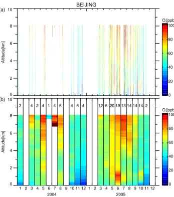
3.1.1 Climatology of ozone profiles over Beijing observed by MOZAIC airborne measurements

Ozone profiles over Beijing have been obtained by MOZAIC airborne measurements taken from March 1995 through November 2005. We fully analyzed the ozone profiles over Beijing for the entire period, and here we present the data in 2004 and 2005 when

5

OMI data are also available. Figure 1a shows the daily values of the ozone mixing ra-tio (in ppbv) observed by MOZAIC measurements over Beijing in 2004 and 2005, and Fig. 1b shows their monthly mean values. For most days, measurements were con-ducted twice daily; the daily averaged values for the two measurements are shown in Fig. 1a. Numbers of the data used for each month are shown in Fig. 1b. Some profiles

10

do not cover all altitudes, as shown in the figure; thus, the numbers of the data de-pended on altitude for some months. Above 6 km in altitude, the mixing ratio was often

as high as 80 to 100 ppbv, as shown in July 2005, which clearly indicates the effects

of stratospheric ozone intrusion. During the period of March 1995 to November 2005,

we found that the effects of ozone intrusion from the stratosphere were sometimes

15

remarkable over Beijing. Ozonesonde measurements revealed similar features over Sapporo and Tsukuba in winter and early spring every year (Nakatani et al., 2012). In June 2005 enhancement of the lower tropospheric ozone (< 2 km) was remarkable. Because the minimum ozone mixing ratio was also clearly detected at around 4 km in altitude, we concluded that enhancement of the lower tropospheric ozone was not

con-20

nected to stratospheric ozone intrusion into the lower troposphere. Rather, the ozone enhancement can be regarded as being derived from ozone production in the lower troposphere. A typical example is shown in greater detail in the following section.

3.1.2 A typical example of significant enhancement of lower tropospheric ozone observed on 22 June 2005

25

(12)

ACPD

15, 2013–2054, 2015

S. Hayashida et al.

Title Page

Tables Figures

◭ ◮

Back Close

Full Screen / Esc

Discussion

P

a

per

|

Discussion

P

a

per

|

Discussion

P

a

per

|

Discussion

P

a

per

|

of ozone was observed on that day. The ozone in the boundary layer as observed at 10:41 was about 120 ppbv and increased to about 190 ppbv at the peak altitude

at 14:18. The profiles of CO, H2O, and temperature are also shown with the ozone

profile in the figure. A CO enhancement of up to 1 ppmv is also clearly visible in the figure, corresponding to ozone enhancement in the boundary layer (< 2 km). However,

5

there was no sign of tropopause folding in the temperature and H2O profiles on that

day. These measurements clearly indicate that the enhancement of ozone at a lower altitude (< 2 km) is not attributed to intrusion of stratospheric ozone, but rather to ozone production in the boundary layer.

In Fig. 2, OMI-derived ozone data for the three layers (22nd, 23rd, and 24th) in the

10

troposphere are also shown with the a priori data. For comparison with the coarse res-olution OMI data, the MOZAIC ozone profile, which originally had a 150 m resres-olution, was averaged for the corresponding layers. In the 24th layer, the OMI retrieval was sig-nificantly lower than the corresponding smoothed-MOZAIC ozone value but was higher

than the a priori value. In the upper two layers, OMI retrievals did not differ significantly

15

from the smoothed-MOZAIC ozone values but were slightly higher than the a priori. In the following section, we compare the OMI retrievals with MOZAIC measurements obtained in 2004 and 2005 in greater detail.

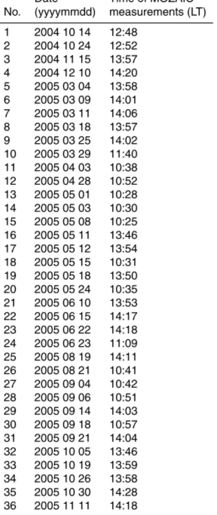
3.1.3 Validation of OMI-derived ozone by MOZAIC measurements

We selected the OMI data at the grid including Beijing from the same day as the

20

MOZAIC measurements were conducted. As described in Sect. 2, all OMI data were prescreened by the criteria of ECF and RMS. When multiple data were available on the same day, we selected the data closer to 13:45. Finally, we chose 36 profiles in 2004 and 2005, which are listed in Table 1. To compare the OMI and MOZAIC ozone data, we accumulated the MOZAIC data of about 150 m resolution to adjust to the coarse

25

OMI-retrieved ozone layers.

(13)

ACPD

15, 2013–2054, 2015

S. Hayashida et al.

Title Page

Tables Figures

◭ ◮

Back Close

Full Screen / Esc

Discussion

P

a

per

|

Discussion

P

a

per

|

Discussion

P

a

per

|

Discussion

P

a

per

|

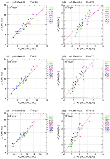
the 22nd, 23rd, and 24th layers, respectively. The linear regression equation of best fit

is shown above each panel with a coefficient of determination, known as theR2value.

Although OMI ozone retrievals considerably underestimate ozone concentrations, a

good linearity was recognized because theR2values were as large as 0.68 at the 24th

layer. Good correlation was present partly because the a priori data implicitly involve

5

seasonal variation. The data shown in Fig. 3 are color coded according to month; seasonal variations with highs during the summer and lows in winter are notable in

both the MOZAIC ozone data and OMI retrievals. To avoid this effect on evaluating the

correlation, we also show correlations between the differences from the a priori values.

Here, we denote MOZAIC ozone asX and the a priori data as X_a. The∆O₃of OMI is

10

defined as O₃(retrieval)₋X_a, as mentioned in Sect. 2. The three panels in the middle

of Fig. 3 show correlation betweenX₋X_a (MOZAIC) and∆O3 (OMI). The values of

∆O3(OMI) follow the large variability ofX−Xa(MOZAIC) with good linearity, reflecting

frequent enhancements of ozone in the 24th layer. On the contrary, correlations were

weaker in the other two layers because the variations of X₋X_a (MOZAIC) in those

15

layers were significantly smaller than those in the 24th layer. However, the effects from

other layers are significant because of large smoothing errors in the OMI retrievals and examination of the AKs is required.

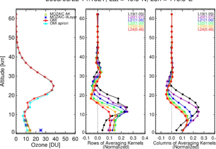
Figure 4 shows the AKs on 22 June 2005 for rows (middle) and columns (right). The profiles of the a priori and OMI-retrieved ozone are shown in the left panel. The middle

20

panel shows profiles of the rows of AKs that are normalized by the a priori error (Liu et al., 2010a) for the six layers (layers 19–24) of OMI retrieval. The right panel shows similar profiles but for the columns of AKs. The rows and columns of AKs for each layer indicate the sensitivity of retrieved ozone at this layer to actual ozone change at all layers, and the sensitivity of retrieved ozone at all layers to actual ozone change at this

25

layer, respectively. The total retrieval e_fficiency shown in parentheses in the legend is

defined as the sum of the column of AKs for each layer. The total retrieval efficiency at a

specific layer indicates the fraction of actual ozone change at the layer in the total of the

(14)

ACPD

15, 2013–2054, 2015

S. Hayashida et al.

Title Page

Tables Figures

◭ ◮

Back Close

Full Screen / Esc

Discussion

P

a

per

|

Discussion

P

a

per

|

Discussion

P

a

per

|

Discussion

P

a

per

|

almost 50 % of the ozone enhancement from the bottom layer can be retrieved. The columns of AKs indicate that retrieval response to the actual enhancement of ozone at 24th layer does not necessarily peak at the 24th layer, but also at upper layers. However, the enhancement of ozone at upper troposphere such as that at the 21st or 22nd layer does not lead to a peak at the 23rd or 24th layer. Therefore, identification of

5

the peak layer of the ozone profile in the OMI retrieval is useful for distinguishing the cause of ozone enhancement.

In the rightmost panels of Fig. 3, we show the correlation betweenX₋X_a(MOZAIC)

at the 24th layer and the ∆O3 (OMI) of the 22nd layer (c1), or the ∆O3 (OMI) of the

23rd layer (c2). These two panels show better correlation than that with the same layer

10

as in (b2) and (b3), which indicates that the e_ffect of enhancement of ozone at the 24th

layer could propagate to the upper layers. In panel (c3), we also show the correlation

betweenX₋X_a (MOZAIC) at the 24th layer and the summation of ∆O3 (OMI) of the

23rd layer and of the 24th layer.

To confirm the consistency in the OMI ozone retrievals, we applied OMI AKs (rows)

15

to the MOZAIC data by using the following equation:

X_j′₌X_a,_j₊

n X

i=1

A(i,j) [X_t,_iX_a,_i], (1)

whereX′

j is the MOZAIC ozone profile convolved with the retrieval AKs (A(i,j)), Xt is

the MOZAIC ozone profile on the OMI altitude grid, andX_a is the a priori profile used

in the OMI retrievals. Here, n=24, and j=24 for the 24th layer of the OMI ozone.

20

We applied Eq. (1) to MOZAIC measurements only for i ₌22, 23, and 24, and we

assumed X_t as the OMI-retrieved data for the other layers above (i ₌1, 21) because

of the unavailability of measurement data. The ozone values (X_t) on 22 June 2014 are

shown in the left panel of Fig. 4.

After applying Eq. (1), we compared the MOZAIC and OMI-retrieved ozone for the

25

(15)

ACPD

15, 2013–2054, 2015

S. Hayashida et al.

Title Page

Tables Figures

◭ ◮

Back Close

Full Screen / Esc

Discussion

P

a

per

|

Discussion

P

a

per

|

Discussion

P

a

per

|

Discussion

P

a

per

|

36 days are color coded in the figure according to month, similar to those in Fig. 3. As previously mentioned for Fig. 3, the strong correlation is partly due to the retrieved ozone variation accompanied by the seasonal variation involved in the a priori values.

Then, we again compared∆O₃with MOZAIC in a similar fashion. The rightmost panels

in Fig. 5b1, b2, and b3 show scatter plots ofX′

−Xa derived from MOZAIC

measure-5

ments and∆O3from OMI data. The correlation ofX′−Xawith ∆O3shown in Fig. 5b

was also evaluated to be sufficient, although the fitting line indicated slight

overesti-mation by the OMI in the 23rd and 24th layers; the slope coefficients of∆O3 (by OMI)

againstX′

−Xa(by MOZAIC) were approximately 0.9, 1.3, and 1.4 for the 22nd, 23rd,

and 24th layers, respectively. All of the results shown in Fig. 5 assure the validity of

10

OMI retrievals.

3.2 Global distribution of∆O3

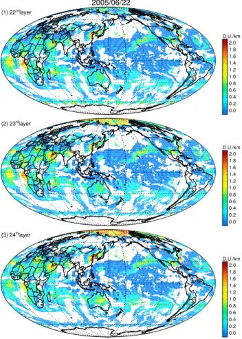
In the previous section, we demonstrated the validity of OMI retrievals. In this section, we show an unusual ozone enhancement over the CEC as compared with other

ar-eas. Figure 6 shows global maps of OMI∆O₃ observed on 22 June 2005. Panels (1),

15

(2), and (3) depict the 22nd, 23rd, and 24th layers, respectively. To make all data on the same scale, we divided the original ozone amount in DUs by the layer thickness;

thus, all data in Fig. 6 are in D.U. km−1_{. It is obvious that the high values of}

∆O3 are

remarkable only over the CEC, with the exception of the Arabian Peninsula near Qatar

and tropical Africa. There was no systematic distribution of high∆O3 in the same

lati-20

tudinal regions in which the solar zenith angle was similar, which demonstrates that the enhancement of ozone is not an apparent phenomenon due to the change in retrieval

efficiency depending on solar zenith angle. The screening process according to the

criteria of ECF and RMS, as described in Sect. 2, resulted in an absence of data in some areas.

25

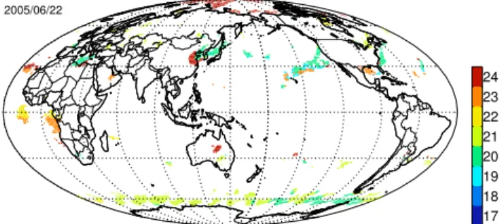
To investigate the altitude of the ozone enhancement in greater detail, we show in

Fig. 7 the peak layer of∆O3, hereafter referred to as the layer peak, at the grids in which

(16)

ACPD

15, 2013–2054, 2015

S. Hayashida et al.

Title Page

Tables Figures

◭ ◮

Back Close

Full Screen / Esc

Discussion

P

a

per

|

Discussion

P

a

per

|

Discussion

P

a

per

|

Discussion

P

a

per

|

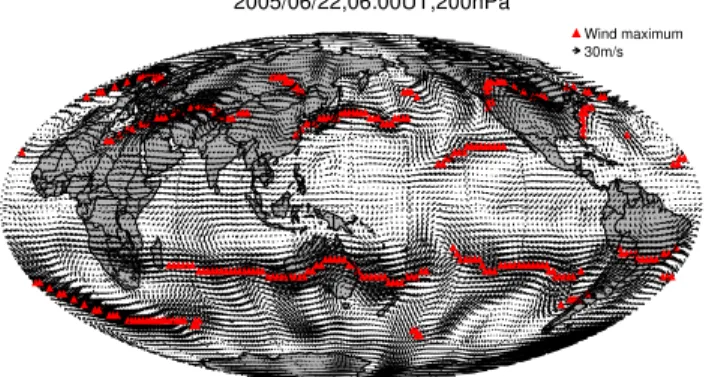
global map of NCEP wind at 200 hPa on the same day with the location of the maximum wind speed indicating STJ. Over the CEC the layer peaks appeared at the 24th layer, which demonstrates that the ozone enhancement occurred in the lower troposphere over CEC rather than in the upper troposphere. We will discuss relationships between

∆O3and STJ in Sect. 4.

5

3.3 Correlation with MOPITT CO and MODIS hotspots over East Asia

In this section, we present relationships between the lower tropospheric ozone en-hancements and biomass burning activity. As described in Sect. 1, recent studies have

revealed a significant effect of OCRB after the harvest of winter wheat on ozone

produc-tion in June over the CEC (Kanaya et al., 2013). In Fig. 9, we show East Asian maps

10

of the a priori values,∆O₃, and retrieved ozone observed by OMI in the 22nd layer,

23rd layer, and 24th layer on 22 June 2005. The ozone enhancement was clearly visi-ble over Shandong and the North China Plain. For comparison with lower tropospheric ozone enhancements, we also show in Fig. 10a and c the CO distribution observed from MOPITT and the hotspot numbers taken from MODIS obtained on the same day,

15

respectively. The areas in which significant hotspots were found correspond to CO and ozone enhancements. This result obtained from OMI is consistent with that in previous

studies of MTX2006 that investigated the e_ffect of OCRB on ozone production. This

fact indirectly confirms the validity of OMI products.

3.4 Annual and inter-annual variation of ozone distribution in the lower

tropo-20

sphere

Figure 11 shows the monthly mean value of the OMI-retrieved ozone from January to December 2005 at the 24th layer. It should be noted that the monthly mean map shown in Fig. 11 is not synoptic; rather, it is a composite of patchy measurements made under clear-sky conditions only. However, more than half (> 15) of the data were generally

25

(17)

ACPD

15, 2013–2054, 2015

S. Hayashida et al.

Title Page

Tables Figures

◭ ◮

Back Close

Full Screen / Esc

Discussion

P

a

per

|

Discussion

P

a

per

|

Discussion

P

a

per

|

Discussion

P

a

per

|

Figure 11 shows obvious ozone enhancement in the lower troposphere in June. The layer peak data were also investigated in June 2005. The most frequent layer peak in June 2005 occurred in the 24th layer over the CEC. This result supports that the ozone enhancement observed in June, other than the typical example day of 22 June, can be attributed to the lower troposphere and not to the upper troposphere. The results

5

shown in Fig. 11f are comparable with those in Fig. 10b and d, and the region of ozone enhancement is also strongly connected to CO and hotspots on a monthly basis.

Figure 12 shows the monthly mean value of the retrieved ozone at the 24th layer in June from 2005 through 2013. The year-to-year variability is significant; however, the spatial distribution pattern is similar every year, whereby a region of high ozone

10

concentration appears around the Shandong Peninsula. The maps after 2009 had rel-atively noisy features due to inferior data quality and reduced spatial coverage after the severe row anomaly problem in 2009. However, despite some noisy patterns shown in the maps after 2009, the characteristic feature of ozone enhancement can be rec-ognized every year. The data numbers shown in the Supplement (Fig. S3) reveal that

15

most of the grid are covered by more than 15 data.

4 Discussion

4.1 Sensitivity of the OMI ozone retrieval scheme to the lower troposphere

Liu et al. (2010a) reported that although the tropospheric degree of freedom for the signal (DFS) for clear-sky conditions typically peaks in the 500–700 hPa layer (i.e.,

20

layer 23) and the DFS in the lower troposphere is generally small, the retrieval effi

-ciency for the lowermost layer is typically 0.4–0.7 for most tropical and mid-latitude summer conditions due to the small solar zenith angles. This indicates that 40–70 % of the actual ozone change from the a priori in the 24th layer can be retrieved although not necessarily at the same layer due to smoothing. For the grid including Beijing shown

25

(18)

ACPD

15, 2013–2054, 2015

S. Hayashida et al.

Title Page

Tables Figures

◭ ◮

Back Close

Full Screen / Esc

Discussion

P

a

per

|

Discussion

P

a

per

|

Discussion

P

a

per

|

Discussion

P

a

per

|

slightly peaked at layer 24, although no significant difference was shown in the

lower-most five layers, and the total retrieval efficiency for layer 24 was 0.46.

Although Liu et al. (2010b) also reported validation of OMI ozone profiles between 0.22 and 215 hPa and a stratospheric ozone column decrease to 215 hPa against

v2.2 MLS data from 2006, validation for the lowermost altitude has not been sufficiently

5

studied. The validation of OMI ozone retrieval for the lowermost troposphere under con-ditions of significantly enhanced ozone, such as those observed over the CEC, has not been evaluated prior to this study because only limited ozone profile data over China are available. In this study, we utilized MOZAIC airborne measurement data and ex-amined the possibility of lower tropospheric ozone detection from OMI over Beijing in

10

detail, although the data were limited to the period before November 2005. In Sect. 3.1, we compared the OMI-retrieved ozone data with MOZAIC airborne data over Beijing. We presented in Fig. 2 a typical ozone profile showing significant enhancement in the lower troposphere, and we showed other related results concerning this case.

In addition to the aforementioned case of 22 June 2005, we selected 36 coincident

15

pairs of OMI and MOZAIC data as listed in Table 1, and we compared them in Fig. 3. A direct correlation between the MOZAIC and OMI ozone data showed good linearity,

withR2₌0.68 for the 24th layer (Fig. 3a3). However, the a priori data implicitly involve

seasonal variation, and the good correlation shown in Fig. 3a was partly caused by large seasonal variation. Therefore, the observed correlation in Fig. 3a does not assure

20

reliability of OMI ozone retrievals. To avoid this effect on the correlation evaluation, we

also showed correlations between the differences from the a priori values,X₋X_aand

∆O₃, in Fig. 3b.

For the lowermost 24th layer, large values ofX₋X_a(up to 15 DU) were observed by

MOZAIC (Fig. 3b3). The OMI retrievals at the 24th layer significantly underestimated

25

the ozone because some of ozone enhancement was retrieved at upper layers, and some could not be retrieved due to reduced photon penetration into the lower

tropo-sphere. The regression coefficient of OMI ozone was 0.17 against MOZAIC ozone. On

(19)

ACPD

15, 2013–2054, 2015

S. Hayashida et al.

Title Page

Tables Figures

◭ ◮

Back Close

Full Screen / Esc

Discussion

P

a

per

|

Discussion

P

a

per

|

Discussion

P

a

per

|

Discussion

P

a

per

|

indicator for relative changes of ozone in the lower troposphere, although the absolute values are considerably underestimated.

The AKs used to retrieve ozone profiles of 22 June 2005 are shown in Fig. 4. These

profiles suggest that it is difficult to independently distinguish the lower three

tropo-spheric layers. On the contrary, the AK profile of the 24th layer also shows that the OMI

5

retrieval scheme is sensitive to the lowermost layer with a total retrieval efficiency of

0.46 even though the DFS of 0.11 at this layer is not sufficiently large. However, we

should also note that when the lowermost ozone increases, the ozone at the 22nd and 23rd layers is also enhanced, as shown in Figs. 2 and 6.

In the 22nd and 23rd layers, the variation in ozone quantities observed by MOZAIC

10

was less than that in the 24th layer; thus, the correlation between MOZAIC and OMI was unclear. As shown in Fig. 3b1 and b2, the ozone data were scattered almost randomly about the zero-point for the 22nd and 23rd layers. In the rightmost panels

of Fig. 3, we show the correlation between X₋X_a (MOZAIC) at the 24th layer and

∆O3(OMI) of the upper layers. The correlation in (c1) and (c2) is more significant than

15

that with the same layer as in (b1) and (b2). As indicated in the columns of AKs in Fig. 4 (right), the actual enhancement of ozone at the 24th layer does not necessarily appear at the 24th layer but is expected to peak at one or two layers higher. In Fig. 3c3,

we show the correlations betweenX₋X_a(MOZAIC) at 24th layer and∆O3(OMI) values

for the summation of the two layers at 23 and 24. The correlations are in a reasonable

20

range when we consider the large smoothing errors.

Figure 5 indicates good consistency of OMI retrievals for both ozone and∆O3.

Vali-dation including stratospheric data, with ozonesonde data provided by Y. Wang (Wang et al., 2012) in Beijing, is currently under study and will be reported in our next paper.

4.2 E_ffects of stratospheric ozone intrusion

25

In Fig. 6, we show the distribution of ∆O3 in D.U. km−

1

at each layer because the AKs are based on the DU of the ozone amount. If we present these figures in mixing

(20)

ACPD

15, 2013–2054, 2015

S. Hayashida et al.

Title Page

Tables Figures

◭ ◮

Back Close

Full Screen / Esc

Discussion

P

a

per

|

Discussion

P

a

per

|

Discussion

P

a

per

|

Discussion

P

a

per

|

can provide a misleading interpretation because air density is significantly lower in the upper layers. In fact, the absolute ozone amount is higher in the lower troposphere even if the mixing ratio is lower.

Despite the difficulty in distinguishing ozone in the first three layers based on the

rows of AKs (middle panel of Fig. 4), the columns of AKs (or the retrieval efficiency, right

5

panel of Fig. 4) provide useful information about the likely source of ozone

enhance-ment. As shown in Fig. 4, the retrieval efficiency curve to actual ozone enhancement

in the lowermost layer tends to peak at layer 22 or lower, whereas the curve to actual ozone enhancement from stratospheric intrusion tends to peak at higher altitudes (e.g., layers 19 and 20). Therefore, the peak layer of ozone retrieval enhancement can help

10

to discriminate the likely sources of ozone enhancement between stratospheric intru-sion and the lowermost troposphere, especially when there is significant tropospheric ozone enhancement. Figure 7 shows the layer of peak tropospheric ozone enhance-ment for nearly clear-sky pixels. Over China, the peak layer was at layer 24, suggesting that the ozone enhancement was very likely from the lowermost troposphere. In

con-15

trast, the peak layer over the East Pacific occurred mostly in layers 19–20, suggesting the stratosphere as a likely origin as confirmed by the location of subtropical jet shown in Fig. 8.

The OMI 22nd layer was lower than 9 km and often lower than ∼8 km (Fig. 2); the

layer was significantly lower than the tropopause, particularly in the summer. Therefore,

20

the OMI tropospheric ozone specifically at layers 22–24 studied was significantly lower in altitude than the tropopause. Nevertheless, as mentioned in Sect. 1, awareness of stratospheric ozone intrusion is needed because ozone enhancement in the upper

tro-posphere/lower stratosphere affects lower tropospheric ozone retrieval, as shown by

the AKs displayed in Fig. 4. To avoid stratospheric effects, we analyzed and compared

25

global maps of_∆O₃in the troposphere (Fig. 6) with the NCEP wind data (Fig. 8) to

in-vestigate their relationship. Notably high∆O3was found in only a few regions, including

(21)

ACPD

15, 2013–2054, 2015

S. Hayashida et al.

Title Page

Tables Figures

◭ ◮

Back Close

Full Screen / Esc

Discussion

P

a

per

|

Discussion

P

a

per

|

Discussion

P

a

per

|

Discussion

P

a

per

|

during the entire observation period from 2004 to 2013, and we surveyed all of the data

(figure not shown). With this visual examination, we found no correlation between∆O3

in the 24th layer and the location of the subtropical jet.

4.3 Effects of OCRB in June over the CEC

In the CEC, an unusually high rate of ozone production could be attributed to

emis-5

sions of anthropogenic ozone precursors such as NOx, CO, and VOCs. High

concen-trations of NOx in the CEC are well known from satellite measurements (e.g., Richter

et al., 2005). In addition to those from emissions of industrial activities and automobile

exhaust, recent studies revealed significant effects on ozone production by emissions

derived from agricultural activities in June, especially OCRB after the harvesting of

10

winter wheat. Fu et al. (2007) used a six-year record (1996 to 2001) of GOME satellite HCHO measurements, and investigated regional emissions over South Asia and East Asia. They revealed a large source to be agricultural burning in the North China Plain in June, which is not included in current bottom-up inventories.

In 2006, Japanese and Chinese researchers jointly conducted a field campaign,

15

MTX2006, at Mt. Tai (36.26◦_{N, 117.11}◦_{E, 1534 m a.s.l.) in Shandong Province,}

lo-cated at the center of the CEC, during the period of 28 May to 30 June 2006. The results of the campaign were published in the special issue of Atmospheric Chem-istry and Physics under “The Mount Tai Experiment 2006 (MTX2006): regional ozone photochemistry and aerosol studies in Central East China” with an overview paper by

20

Kanaya et al. (2013). In the campaign, the team measured O₃, CO, NO_x, NO_y, and

aerosol components simultaneously (Table 3 of Kanaya et al., 2013) and observed an unusual ozone increase of up to 160 ppbv in early and mid-June at Mt. Tai (Fig. 3 of Kanaya et al., 2013). This ozone enhancement was accompanied by an increase in

CO and other VOCs, which substantiated the effects of biomass burning. In this region,

25

(22)

ACPD

15, 2013–2054, 2015

S. Hayashida et al.

Title Page

Tables Figures

◭ ◮

Back Close

Full Screen / Esc

Discussion

P

a

per

|

Discussion

P

a

per

|

Discussion

P

a

per

|

Discussion

P

a

per

|

the high concentrations of O₃, and its precursors and aerosols, in June was

identi-fied as regional-scale OCRB after the harvesting of winter wheat. Kanaya et al. (2013) presented photographs of smoky scenery captured at the observation site. They stated that the composition at the field site was strongly influenced by large-scale post-harvest OCRB of winter wheat.

5

The ozone enhancement observed in June 2006 by MTX2006 was consistent with the OMI results we presented in this study. We examined a time series of OMI-derived

ozone at the grid including that at Mt. Tai (36.26◦_{N, 117.11}◦_{E) at the 24th layer}

dur-ing the period of the MTX2006 campaign. Applydur-ing the linearity shown in Fig. 3b3, we

converted the original OMI retrieval as∆O₃/ 0.17+X_a, where 0.17 is the linear

regres-10

sion coe_fficient. We found that the scale of ozone enhancement up to about 140 ppbv

was roughly consistent with that observed in MTX2006, supporting the reliability of the OMI-derived ozone data shown in the present study.

4.4 Suggestions for future study

Ozone enhancement was most notable in June of every year, as presented in Fig. 11.

15

Some model studies were published in the MTX2006 special issue. Li et al. (2008) used a 3-D regional chemical transport model, known as the Nested Air Quality Model System (NAQPMS). They presented the simulated monthly mean near-ground ozone (Fig. 5 of Li et al., 2008), which is comparable to that in Fig. 12b in the present study. Yamaji et al. (2010) used the Model-3 Community Multiscale Air Quality Modeling

Sys-20

tem (CMAQ) to investigate the e_ffects of OCRB with daily gridded emissions by

ap-plying the bottom-up method. They presented daily ozone maps (Fig. 8 of Yamaji et al., 2010), which are also comparable to the OMI daily maps obtained by the present study. The comparison of OMI-derived ozone maps with multiple-mode simulations can lead to a better understanding of emissions from crop burning, which is an important

25

topic for further investigation.

The ozone maps shown in Figs. 11 and 12 indicate that the maximum _∆O₃ value

(23)

ACPD

15, 2013–2054, 2015

S. Hayashida et al.

Title Page

Tables Figures

◭ ◮

Back Close

Full Screen / Esc

Discussion

P

a

per

|

Discussion

P

a

per

|

Discussion

P

a

per

|

Discussion

P

a

per

|

from China to Korea and Japan. Detailed meteorological analysis to reveal the trans-port processes of ozone as investigated by Pan et al. (2013) is currently under study, coupled with the analysis of the ground-based data over Japan taken from the database of Atmospheric Environmental Regional Observation System (AEROS;

http://soramame.taiki.go.jp/). As previously mentioned, it would be difficult to reveal the

5

ozone distribution in East Asia by only the use of ground-based monitoring stations and sea-borne measurements. In this study, we demonstrated the potential of satellite measurements to address this issue. The ozone maps shown in Figs. 11 and 12 will be

helpful for modelers in examining the effects of various emission scenarios on ozone

production and for exploring unknown factors influencing ozone distribution.

10

As discussed in Sect. 4.1, UV radiation measurements are sensitive to ozone in the

lowermost altitudes, although this sensitivity is not sufficiently large. On the contrary,

TIR measurements have more sensitivity to ozone in the mid- and upper troposphere. Combined use of TIR and UV sensors would be helpful for investigating ozone profiles in greater detail, as reported by Safieddine et al. (2013). A prospective synergetic

re-15

trieval algorithm combining UV and TIR should be the subject of future study. Cuesta et al. (2013) applied a multispectral synergetic algorithm with IASI for TIR and GOME-2 for UV radiation. It may be possible to extend their algorithm to couple with the OMI re-trievals shown in the present study. Combined use of OMI and TES, both of which are based on the same platform, and the EOS Aura satellite would also be highly useful,

20

as Fu et al. (2013) demonstrated in their feasibility study. We hope this research will encourage such a synergetic study.

5 Summary

The recent OMI products retrieved by Liu et al. (2010a) revealed spatial and temporal variations in ozone distributions in multiple tropospheric layers. The validation of OMI

25

(24)

ACPD

15, 2013–2054, 2015

S. Hayashida et al.

Title Page

Tables Figures

◭ ◮

Back Close

Full Screen / Esc

Discussion

P

a

per

|

Discussion

P

a

per

|

Discussion

P

a

per

|

Discussion

P

a

per

|

this study because only limited ozone profile data over China are available. We com-pared the OMI-derived ozone over Beijing with airborne measurements conducted by the MOZAIC program, and we examined in detail the possibility of lower tropospheric ozone detection from OMI over Beijing, although the data were limited to the period be-fore November 2005. Under the condition of highly enhanced ozone such as that over

5

Beijing, the correlation between OMI and MOZAIC ozone in the lower troposphere was reasonable, which verified the reliability of OMI ozone retrievals at the lower tro-posphere under enhanced ozone conditions. The ozone enhancement over the CEC was clear in June of every year, which is associated with the enhancement of CO and hotspots. This result suggests that a considerable portion of the enhancement could

10

be attributed to the emissions of ozone precursors from residue burning after the har-vesting of winter wheat in these regions, as investigated by in-situ measurements in MTX2006 (Kanaya et al., 2013).

The lower tropospheric ozone distribution maps were first obtained from OMI retrieval in the present study; these maps are consistent with the results from some model

sim-15

ulations that include OCRB emissions. The OMI-derived information on lower tropo-spheric ozone will be helpful for the investigation of as yet unknown factors influencing ozone distribution by comparison with model simulations. Such a topic is intended for future study.

The Supplement related to this article is available online at

20

doi:10.5194/acpd-15-2013-2015-supplement.

Acknowledgements. We express our thanks to the European Commission for the support to the MOZAIC project (1994–2003), to partner institutions of the IAGOS Research Infrastruc-ture (FZJ, DLR, MPI, and KIT in Germany; CNRS, CNES, and Météo-France in France; and the University of Manchester in the United Kingdom), ETHER (CNES-CNRS/INSU) for

host-25

(25)

ACPD

15, 2013–2054, 2015

S. Hayashida et al.

Title Page

Tables Figures

◭ ◮

Back Close

Full Screen / Esc

Discussion

P

a

per

|

Discussion

P

a

per

|

Discussion

P

a

per

|

Discussion

P

a

per

|

our gratitude to Ms. H. Araki and Ms. M. Nakazawa for their help with the data analysis and creation of figures and to Yugo Kanaya for his helpful comments on MTX2006. S. Hayashida and A. Ono were supported by a Grant-in-Aid from the Green Network of Excellence, Environ-mental Information (GRENE-ei) program, MEXT, Japan. X. Liu and K. Chance were supported by NASA and the Smithsonian Institution.

5

References

Aires, F., Aznay, O., Prigent, C., Paul, M., and Bernardo, F.: Synergistic multi-wavelength remote sensing versus a posteriori combination of retrieved products: Application for the retrieval of atmospheric profiles using MetOp-A, J. Geophys. Res., 117, D18304, doi:10.1029/2011JD017188, 2012.

10

Chance, K., Palmer, P. I., Spurr, R. J. D., Martin, R. V., Kurosu, T., and Jacob, D. J.: Satellite observations of formaldehyde over North America from GOME, Geophys. Res. Lett., 27, 3461–3464, 2000.

Cuesta, J., Eremenko, M., Liu, X., Dufour, G., Cai, Z., Höpfner, M., von Clarmann,T., Sellitto, P., Foret, G., Gaubert, B., Beekmann, M., Orphal, J., Chance, K., Spurr, R., and

Flaud,J.-15

M.: Satellite observation of lowermost tropospheric ozone by multispectral synergism of IASI thermal infrared and GOME-2 ultraviolet measurements over Europe, Atmos. Chem. Phys., 13, 9675–9693, doi:10.5194/acp-13-9675-2013, 2013.

Deeter, M. N., Worden, H. M., Gille, J. C., Edwards, D. P., Mao, D., and Drummond, J. R.:

MOPITT multispectral CO retrievals: Origins and e_ffects of geophysical radiance errors, J.

20

Geophys. Res., 116, D15303, doi:10.1029/2011JD015703, 2011.

Deeter, M. N., Martínez-Alonso, S., Edwards, D. P., Emmons, L. K., Gille, J. C., Worden, H. M., Pittman, J. V., Daube, B. C., and Wofsy, S. C.: Validation of MOPITT Version 5 thermal-infrared, near-thermal-infrared, and multispectral carbon monoxide profile retrievals for 2000–2011, J. Geophys. Res.-Atmos., 118, 6710–6725, doi:10.1002/jgrd.50272, 2013.

25

(26)

ACPD

15, 2013–2054, 2015

S. Hayashida et al.

Title Page

Tables Figures

◭ ◮

Back Close

Full Screen / Esc

Discussion

P

a

per

|

Discussion

P

a

per

|

Discussion

P

a

per

|

Discussion

P

a

per

|

European Organisation for the Exploitation of Meteorological Satellites (EUMETSAT): GOME-2 Level 1 product generation specification, EPS.SYS.SPE.990011, Darmstadt, Germany, 2006.

Fishman, J. and Larsen, J. C.: Distribution of total ozone and stratospheric ozone in the tropics’ implications for the distribution of tropospheric ozone, J. Geophys. Res., 92, 6627–6634,

5

1987.

Fishman, J., Wozniak, A. E., and Creilson, J. K.: Global distribution of tropospheric ozone from satellite measurements using the empirically corrected tropospheric ozone residual tech-nique: Identification of the regional aspects of air pollution, Atmos. Chem. Phys., 3, 893–907, doi:10.5194/acp-3-893-2003, 2003.

10

Fu, T.-M., Jacob, D. J., Palmer, P. I., Chance, K., Wang, Y. X., Barletta, B., Blake, D. R., Stanton, J. C., and Pilling, M. J.: Space-based formaldehyde measurements as constraints on volatile organic compound emissions in east and south Asia and implications for ozone, J. Geophys. Res., 112, D06312, doi:10.1029/2006JD007853, 2007.

Fu, D., Worden, J. R., Liu, X., Kulawik, S. S., Bowman, K. W., and Natraj, V.: Characterization of

15

ozone profiles derived from Aura TES and OMI radiances, Atmos. Chem. Phys., 13, 3445– 3462, doi:10.5194/acp-13-3445-2013, 2013.

Giglio, L., Descloitres, J., Justice, C. O., and Kaufman, Y. J.: An enhanced contextual fire detection algorithm for MODIS, Remote Sens. Environ., 87, 273–282, doi:10.1016/s0034-4257(03)00184-6, 2003.

20

Gottwald, M. and Bovensmann, H.: SCIAMACHY – Exploring the changing Earth’s atmosphere, Springer, Germany, 2011.

Hayashida, S., Urita, N., Noguchi, K., Liu, X., and Chance, K.: Spatiotemporal variation in tro-pospheric column ozone over East Asia observed by GOME and ozonesondes, SOLA, 4, 117–120, doi:10.2151/sola.2008-030, 2008.

25

IPCC: Climate Change 2007: The Physical Scientific Basis, Contribution of Working Group I to the Fourth Assessment Report of the Intergovernmental Panel on Climate Change, edited by: Solomon, S., Qin, D., Manning, M., Chen, Z., Marquis, M., Averyt, K. B., Tignor, M., and Miller, H. L., Cambridge University Press, Cambridge, United Kingdom and New York, NY, USA, 2007.

30