Credit scoring: comparison of non‐parametric techniques against logistic regression

Credit Scoring: Comparison of Non-Parametric

Techniques against Logistic Regression

Miguel Mendes Amaro

Dissertation presented as partial requirement for obtaining

the Master’s degree in Information Management

ii

NOVA Information Management School

Instituto Superior de Estatística e Gestão de Informação

CREDIT SCORING: COMPARISON OF NON-PARAMETRIC

TECHNIQUES AGAINST LOGISTIC REGRESSION

by

Miguel Mendes Amaro

Dissertation presented as partial requirement for obtaining the Master’s degree in

Information Management, with a specialization in Knowledge Management and

Business Intelligence

Advisor: Prof. Roberto Henriques, PhD

iii

ABSTRACT

Over the past decades, financial institutions have been giving increased importance to credit risk management as a critical tool to control their profitability. More than ever, it became crucial for these institutions to be able to well discriminate between good and bad clients for only accepting the credit applications that are not likely to default. To calculate the probability of default of a particular client, most financial institutions have credit scoring models based on parametric techniques. Logistic regression is the current industry standard technique in credit scoring models, and it is one of the techniques under study in this dissertation. Although it is regarded as a robust and intuitive technique, it is still not free from several critics towards the model assumptions it takes that can compromise its predictions. This dissertation intends to evaluate the gains in performance resulting from using more modern non-parametric techniques instead of logistic regression, performing a model comparison over four different real-life credit datasets. Specifically, the techniques compared against logistic regression in this study consist of two single classifiers (decision tree and SVM with RBF kernel) and two ensemble methods (random forest and stacking with cross-validation). The literature review demonstrates that heterogeneous ensemble approaches have a weaker presence in credit scoring studies and, because of that, stacking with cross-validation was considered in this study. The results demonstrate that logistic regression outperforms the decision tree classifier, has similar performance in relation to SVM and slightly underperforms both ensemble approaches in similar extents.

KEYWORDS

Credit scoring; models comparison; logistic regression; non-parametric models; machine learning; ensemble methods; heterogeneous ensemble

iv

INDEX

1.

Introduction... 1

1.1.

Background and problem identification ... 1

1.2.

Study relevance and motivations ... 2

2.

Literature review ... 4

3.

Experimental design ... 7

3.1.

Credit datasets ... 7

3.2.

Data pre-processing ... 8

3.2.1.

Missing values ... 8

3.2.2.

Outliers and feature engineering ... 9

3.3.

Feature selection ... 11

3.4.

Algorithms overview ... 14

3.4.1.

Single classifiers ... 15

3.4.2.

Ensemble classifiers ... 21

3.5.

Modelling techniques ... 25

3.5.1.

Sample split ... 25

3.5.2.

Class reweight ... 26

3.5.3.

Hyperparameters optimization ... 27

3.6.

Performance evaluation ... 29

3.6.1.

Confusion matrix and profit maximization ... 29

3.6.2.

ROC curve – AUC and GINI index ... 32

3.6.3.

Other performance indicators ... 32

4.

Results and discussion ... 34

4.1.

Detailed results by dataset ... 34

4.2.

ROC curve – AUC analysis ... 35

4.3.

Averaged indicators analysis... 38

4.4.

Financial impact analysis ... 42

4.5.

Global performance assessment ... 44

4.6.

Comparison with results from previous studies ... 45

5.

Conclusion ... 47

6.

Limitations and recommendations for future works ... 48

v

LIST OF FIGURES

Figure 1 - Median monthly income calculated for each age class ... 9

Figure 2 - Outlier treatment for numeric variables (before) ... 9

Figure 3 - Outlier treatment for numeric variables (after) ... 10

Figure 4 - Feature importance analysis (Kaggle dataset) ... 12

Figure 5 - Spearman’s correlation coefficient (Kaggle dataset) ... 13

Figure 6 - AUC by number of features included in the model ... 14

Figure 7 - Linear regression vs logistic regression ... 15

Figure 8 - Linear SVM Classification (Kirchner & Signorino, 2018) ... 18

Figure 9 - Projection of the original input space in a higher dimension space ... 19

Figure 10 - Kernel Machine... 20

Figure 11 - Parallel and sequential ensemble flux (Xia et al., 2017) ... 22

Figure 12 - Random forest ... 23

Figure 13 - Stacking classifier (Mlxtend library) ... 24

Figure 14 - Stacking with cross-validation classifier (Mlxtend library) ... 25

Figure 15 - Train and test split method and cross-validation ... 26

Figure 16 - Over-sampling and Under-sampling techniques ... 27

Figure 17 - Logistic regression confusion matrix (with a 0.5 threshold) ... 30

Figure 18 - Profit curve in logistic regression model (Kaggle dataset) ... 31

Figure 19 - Reconstructed confusion matrix (with the optimum threshold) ... 31

Figure 20 - ROC curve of logistic regression model in Kaggle dataset ... 32

Figure 21 - ROC curves (Kaggle dataset) ... 36

Figure 22 - ROC curves (Japanese dataset) ... 37

Figure 23 - ROC curves (German dataset) ... 37

Figure 24 - ROC curves (Australian dataset) ... 38

Figure 25 - AUC (average) ... 38

Figure 26 - Balanced Accuracy (average) ... 39

Figure 27 - Sensitivity (average) ... 39

Figure 28 - Specificity (average) ... 40

Figure 29 - Precision (average) ... 40

Figure 30 - F-Beta Score (average) ... 41

Figure 31 - Profit/cost by model (Kaggle dataset) ... 42

Figure 32 - Profit/cost by model (Japanese dataset) ... 43

Figure 33 - Profit/cost by model (German dataset) ... 43

Figure 34 - Profit/cost by model (Australian dataset) ... 44

vi

LIST OF TABLES

Table 1 - Overview of ensemble models applications in credit scoring literature ... 6

Table 2 - General description of the datasets ... 7

Table 3 - Outlier treatment (categorical variables with a low number of categories) .. 10

Table 4 - Outlier treatment (categorical variables with a high number of categories) . 11

Table 5 - Optimal number of features by dataset ... 14

Table 6 - Final set of features included in the models ... 14

Table 7 - Hyperparameters (Logistic regression) ... 28

Table 8 - Hyperparameters (SVM with RBF kernel)... 28

Table 9 - Hyperparameters (Decision tree) ... 28

Table 10 - Hyperparameters (Random forest) ... 28

Table 11 - Hyperparameters (Stacking with cross-validation) ... 29

Table 12 - Confusion Matrix structure ... 29

Table 13 - Cost matrix ... 30

Table 14 - Results (Kaggle dataset) ... 34

Table 15 - Results (Japanese dataset) ... 34

Table 16 - Results (German dataset) ... 35

Table 17 - Results (Australian dataset) ... 35

vii

GLOSSARY

Credit Scoring Model – model that expresses the probability of default of a potential borrower according to its characteristics. As a risk management instrument, banks and credit companies use them to protect them from lending money to clients that are not going to pay it back. Parametric Methods – statistic methods where is assumed that data comes from a population that follows a distribution based on a fixed set of parameters.

Non-Parametric Methods – statistic methods that do not rely on the assumption of a fixed set of parameters distribution. Although it also relies on parameters, it is not a fixed set of them, and they are not defined in advance.

“Good” Client – desired client for the bank or credit company that is granting a credit. Client that respects the instalments’ payments.

“Bad” Client – undesired client for the company. Client that does not respect its credit payment obligations, leading to financial losses for the banks or credit companies that lend the money. Dependent or Target Variable – variable that we want to predict. In credit scoring problems, we want to predict if the client is going to default or not.

Independent or Predictor Variables – explanatory variables used to predict the dependent variable.

1

1. INTRODUCTION

1.1. B

Banks and other financial institutions have been giving increased importance to risk management over the last decades. As such, many efforts are made to find more and better instruments to help those institutions in well identifying the several risks and being able to reduce their exposure to it. In particular, credit risk is one of the most significant risks that banks face (Cibulskienė & Rumbauskaitė, 2012). Specialized credit companies and banks, bound to several international regulations (from Basel Committee, for instance) and concerned about being competitive and profitable, are continuously searching for the most appropriate resources and techniques to manage their risk. Moreover, they need the best instruments to accurately tell the probability of a potential client to not pay his loan, at the moment he applies to it. That probability is commonly denominated as the probability of default. There is not a single definition of default since each institution defines its own concept according to its reality and aligned with the specific credit risk problem they are trying to manage. An example of a standard definition of default is the one in the Basel II framework which defines it as being "past due for more than 90 days on any material credit obligation to the banking group” (Basel Committee on Banking Supervision, 2006).

Credit scoring models are instruments used to come up with those probabilities, and they have been gaining popularity over the last decades. Being an instrument that was first used in the 1960s, it can briefly be defined as the use of statistical models to transform relevant data into numerical measures that will guide the credit decision (Anderson, 2007). In order to build a credit scoring instrument, analysts use historical data on the performance of already financed loans to understand what borrowers characteristics are determinant and useful for predicting whether the client will or not default (Mester, 1997). These models have evolved in a significant way over the last years, and in a general overview, they use techniques that allow us to segment them in two groups according to their statistical approach: parametric and non-parametric. Parametric models make assumptions regarding the data they use, such as normal distribution, linearity, homoscedasticity, and independence. On the other hand, the non-parametric models make no assumptions (or at least few). Logistic regression technique belongs to the first group (parametric models). In 2007, (Anderson, 2007) mentioned this technique as the most widely used in the field of credit scoring and (Lessmann, Baesens, Seow, & Thomas, 2015) in their benchmark study still pointed logistic regression as the industry standard technique. Critics exist towards this technique and, they mainly reside in the assumptions it makes and the violation of those same assumptions which can sacrifice the model accuracy.

As an alternative, non-parametric models are becoming more popular aligned with the progress in machine learning which, according to Arthur Samuel in 1959, it consists in giving the "computers the ability to learn without being explicitly programmed". According to studies already performed in the area, these later techniques show superior performance, especially in modelling nonlinear patterns when compared to statistical techniques (Wang, Hao, Ma, & Jiang, 2011). Among the several machine learnings algorithms that currently exist, there is not one that is regarded as the most suitable for credit scoring purpose (Wang et al., 2011). Decision tree algorithms, in particular, have been gaining popularity with the machine learning revolution. This technique uses mathematical formulas like Gini index to find an attribute of the data as well as a threshold value for that attribute to make splits of the input space (Patil & Sareen, 2016). These actions aim to come up, in the end, with different buckets

2

defined by splitting rules and filled with similar instances in terms of their class. Applied to the context of credit scoring, this method will find the splitting rules that efficiently distinguish the bad from the good clients in terms of their probability of default. Decision trees have showed success in solving credit scoring classification problems in several studies (Lee, Chiu, Chou, & Lu, 2006; Ince & Aktan, 2009). Moreover, this technique has a comparative advantage regarding other non-parametric popular methods such as neural networks or support vector machine: its results are rational and easy to interpret. Despite being easy to interpret and already have proven success in risk classification problems, decision trees used in a format of a single classifier have also evidenced propensity to overlearning the training data compromising its generalization capability. This problem, designated as overfitting, seem to be less present when dealing with ensemble models.

Ensemble models are methods where the predictions of a set of single learners are combined. The different existing methods can be grouped in homogeneous ensembles, where a single type of learning algorithm is used to generate the several base agents, and heterogeneous ensembles where different learning algorithms are mixed (Chapman, 2014). Generically, recent literature has been demonstrating that these learning methods, also designated as multiple classifier systems, are superior to single predictors in modelling probability of default (Wang et al., 2011; Lessmann et al., 2015). However, heterogeneous ensembles have not been as frequently approached in credit scoring studies as other techniques mentioned earlier, which makes it more difficult to be certain about their advantages against other techniques such as logistic regression.

1.2. S

Banks and other financial institutions, mostly using logistic regression or other parametric methods may not be taking full advantage of recent progress in machine learning and available non-parametric approaches. This dissertation has the main objective of quantifying the impacts in performance a financial institution can expect from switching its current logistic regression model to a more complex model developed using a non-parametric technique. In fact, this knowledge extension can be seen as a benefit not only for financial institutions, due to the fact that better predictive techniques can result in higher profits, but also for academics.

To achieve the given objective, this dissertation measures the performance of several modelling techniques against logistic regression. Several models’ benchmarks were performed in previous literature and the set of techniques being compared in this particular dissertation reunites more studied predictive techniques with less present in previous works machine learning methods. More concretely, the techniques being compared against logistic regression consist of two popular single classifiers techniques, decision tree and SVM with RBF kernel, and two ensembles approaches. One homogeneous type (random forest) and one heterogeneous type of ensemble approach (stacking with cross-validation).

The relevance of this study to the literature is reinforced by the inclusion, in the pool of algorithms being compared, of a heterogeneous ensemble approach. Comparing to homogeneous ensembles, heterogeneous ensembles are much less frequent in credit scoring studies and that is an important factor for adding value to this dissertation. The heterogenous ensemble technique being used is StackingCVClassifier (from Mlxtend library), which consists of a renewed version of the original StackingClassifier with the difference that uses cross-validation technique to prepare the input data for the meta-classifier, and by doing that, has a stronger overfitting control.

3

Another relevant aspect of this study is the use of four different real-life credit datasets to be able to draw more consistent conclusions (one from Kaggle community and the others from UCI Machine Learning Repository). Moreover, the comparison is enriched with a set of different performance indicators and more adjusted model training and evaluation methods that have in consideration the class imbalance underlying the datasets being used. The models compared were tuned using an efficient hyperparameter tuning technique named RandomizedSearchCV from Scikit-learn library.

4

2. LITERATURE REVIEW

There is a considerable amount of literature that investigates the application of several statistical and machine learning techniques in the context of credit scoring. These models, given the importance they have for credit companies and banks on their risk management strategies, continue being subject of analysis in the literature.

As previously mentioned, logistic regression is still widely used for credit scoring purposes (Abdou, Pointon, & El-Masry, 2008; Hand & Henley, 1997). This method presents an added value when compared to linear regression, as it is more appropriate when we need binary outcomes. Computational developments made it more viable (Anderson, 2007), and financial institutions under Basel II felt a greater incentive to adopt it as estimated probability of default became needed. Its results are considered easy to interpret, and that became of increased importance when regulators started requiring banks to justify their credit application rejections (Qiu, Kandhai, & Sloot, 2010). However, logistic regression, like any other parametric technique, lives with underlying assumptions that, when violated, compromise the model results' credibility (Anderson, 2007). That scenario suggests that research should be conducted to evaluate the relevance of using an alternative approach such as non-parametric techniques once they are regarded as superior to statistical ones when modelling nonlinear features (Wang et al., 2011).

Classification and regression tree (CART) is an example of a non-parametric technique. In relation to logistic regression, it has the comparative advantage of being able to capture nonlinear relationships between input variables. Classification and regression tree models have showed success in solving credit scoring problems throughout the literature. A study from (Lee et al., 2006) performed credit scoring tasks using CART and MARS models against other techniques. Results have demonstrated that CART and MARS models outperformed discriminant analysis, logistic regression, neural networks and support vector machine by reaching a superior average classification rate. Additionally, an experiment from (Ince & Aktan, 2009) compared CART, neural networks, logistic regression and discriminant analysis techniques in terms of accuracy and CART demonstrated the highest average classification rate. On the other hand, error Type II was also measured, and, in that case, neural networks outperformed the other three models. This aspect is particularly relevant in credit scoring context given that this type of error results in higher misclassification costs when compared with Type I error. Support vector machine is an example of another popular non-parametric technique. Despite being an accurate nonlinear approach, with historical data of large dimension, it can become very computationally expensive. In response to that, (Harris, 2015) assessed the performance of clustered support vector machine and obtained well-compared performances (in relation to support vector machines) in terms of accuracy combined with a relatively cheap computational effort. Along with neural networks, support vector machine algorithms are considered as “black box” models due to the lack of information regarding the relationships between variables (Qiu et al., 2010). CART model has an advantage regarding this issue as it produces results which are easy to interpret. In the particular context of credit scoring, this aspect remains critical as "black-box" models are seen with suspicion and scepticism in the banking sector (Khandani, Kim, & Lo, 2010). On the other hand, it appears to be consensual in the literature about applications of credit scoring modelling techniques that decision trees are prone to overfit. (Zakirov, Baxter, Bartlett, & Frean, 2015) (L, Natarajan, Keerthana, Chinmayi, & Lakshmi, 2016) (Bach, Zoroja, Jakoviü, & Šarlija, 2017).

5

The relatively recent machine learning revolution brought a renewed interest in finding new methods of classification and the ensemble methods have been drawing attention from researchers. These methods seem to help in controlling the problem of overfitting associated with the decision trees models. In fact, (Hu et al., 2006) performed an experimental comparison of several ensemble methods (BaggingC4.5, AdaBoostingC4.5, and random forest) against the C4.5 model. All ensemble methods outperformed the C4.5 single classifier, demonstrating a significantly higher accuracy. In more recent literature, (Chopra & Bhilare, 2018) also compared ensemble tree learning techniques with the single learner decision tree and the empirical analysis showed that the ensemble technique gradient boosting outperformed the single tree classifier.

Regarding ensemble methods, one can classify them in two groups, homogeneous and heterogeneous, depending on if these are formed using a single classification algorithm or if they mix several ones. Although homogeneous ensembles use a single classification algorithm, their base learners are trained using different parts of the dataset or using different feature sets. For example, bagging, boosting and staking are well-known ensemble approaches for modifying the training dataset on credit scoring problems (Wang, Hao, Ma, & Jiang, 2011). Interested in comparing these different approaches of using the dataset in ensemble methods, Dietterich (2000) studied the performance of three methods (Randomizing, Bagging and Boosting) and Boosting returned the best results in most of the tasks assessed. However, it was also evident that under noisy data environment Bagging was the best. Later, Caruana & Niculescu-Mizil (2006) performed an empirical comparison between ten supervised learning methods, in which the boosted trees also demonstrated to be the best learning algorithm overall, and the random forests (bagging method) were the second best. On the contrary, (Lessmann, Baesens, Seow, & Thomas), in 2015, performed an update to the study of (Baesens et al., 2003), in which both single and ensemble classifiers were compared and in the specific family of homogeneous ensembles, random forest had the strongest performance, being superior, among others, to boosted trees.

It is not uncommon to find articles demonstrating ensemble classifiers outperforming logistic regression. However, it is also not difficult to find in the literature that these models do not beneficiate of logistic regression’s great advantage of being easy to interpret. As an example, (Hue, Hurlin, & Tokpavi, 2017) state that logistic regression underperforms ensemble models such as random forest due to its pitfalls in modelling nonlinear effects, but then, on the other hand, random forest prediction technique lacks parsimony, i.e. uses many parameters, which make the model less relevant in credit scoring applications where decision-makers need interpretable rules. Concerned with the subject of lacking interpretability to advanced machine learning techniques, these authors (Hue et al., 2017) studied the possibility of improving logistic regression model with nonlinear decision trees effects. They have discovered that the resulting model outperformed traditional logistic regression while being competitive with random forest achieving an efficient trade-off between performance and interpretability. In a similar line of thought, (Vanderheyden & Priestley, 2018), underline the importance of models developed in a regulated industry to be interpretable and rational. Once that is not always the scenario associated with machine learning algorithms, they have proposed a methodology that blends logistic regression with a core model enhancement strategy. In practice, it was created an ensemble that uses a linear combination of predictions from a set of logistic regression models. The fact of using a linear combination of predictions is referred to as the critical point to achieve the interpretability and rationality required in regulated industries.

6

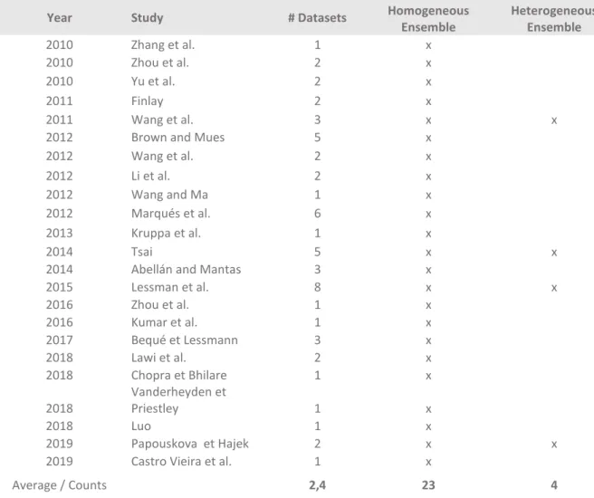
While homogeneous ensemble methods mostly combine the predictions of the base learners by simple or weighted voting, the heterogeneous ensemble models present more complex methods to combine the base learners’ predictions. One of them is stacking and (Dzeroski & Bernard, 2011), through comparing several approaches of it, have shown that this approach achieves improved performance gains in relation to pick the best classifier from the ensemble cross-validation. Regarding the comprehensive benchmark study performed by (Lessmann et al., 2015), heterogeneous ensembles have demonstrated higher performance, but still, it is a field yet to be explored in the literature as table 1 suggests. The table sums up the literature over the last ten years related with applications of ensemble methods in the credit scoring field, and it is clear that homogeneous ensembles have been more present in the several studies and heterogeneous ensemble more neglected. Likewise, table 1 reveals that most of the studies have used one or two datasets to draw conclusions of the modelling techniques which compromises the reliability and consistency of conclusions made.

Year Study # Datasets Homogeneous Ensemble Heterogeneous Ensemble 2010 Zhang et al. 1 x 2010 Zhou et al. 2 x 2010 Yu et al. 2 x 2011 Finlay 2 x 2011 Wang et al. 3 x x

2012 Brown and Mues 5 x

2012 Wang et al. 2 x 2012 Li et al. 2 x 2012 Wang and Ma 1 x 2012 Marqués et al. 6 x 2013 Kruppa et al. 1 x 2014 Tsai 5 x x

2014 Abellán and Mantas 3 x

2015 Lessman et al. 8 x x 2016 Zhou et al. 1 x 2016 Kumar et al. 1 x 2017 Bequé et Lessmann 3 x 2018 Lawi et al. 2 x 2018 Chopra et Bhilare 1 x 2018 Vanderheyden et Priestley 1 x 2018 Luo 1 x 2019 Papouskova et Hajek 2 x x

2019 Castro Vieira et al. 1 x

Average / Counts 2,4 23 4

7

3. EXPERIMENTAL DESIGN

This chapter focus on describing the methodology carried in this study. Firstly, basic information concerning the four real-life datasets is presented. Then, follows an explanation concerning the methods used for data pre-processing and feature selection. Afterwards, there is a concise description of each of the algorithms being compared in this study. Specificities of the modelling work are detailed after as well as the indicators and analysis performed to enable the comparison of the several models developed across the four datasets.

3.1. C

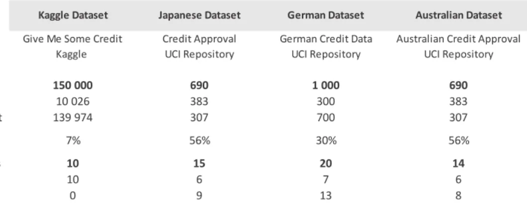
In this dissertation, four real-world credit datasets were used to train and test all the models. The “Give Me Some Credit” dataset referred in this dissertation as the Kaggle Dataset was the dataset used in of the competitions launched by the Kaggle community, a community of data scientists owned by Google, Inc. The other three datasets (referred in this dissertation as the Japanese, German and Australian datasets) are from the UCI Machine Learning Repository and were used several times in previous works (Baesens et al., 2003; Lessmann et al., 2015; Wang et al., 2011). All the four datasets reflect a typical credit scoring classification problem where the variable being predicted distinguishes between desired and undesired credit clients (non-default and default cases respectively). As can be observed in table 2, the Kaggle dataset is by far the largest one of the four, containing 150 thousand of records, whereas the other three have a thousand records maximum. In terms of balance between the two classes of the target variable (default and non-default), the Kaggle dataset is also the most imbalanced one (only 7% of default records), followed by the German Dataset (30% of default records) and then the Australian and Japanese dataset, that are not far from being perfectly balanced (56% of default records).

The features of the datasets combine social with behavioural information (as a client of a credit product) concerning each individual client. This characteristic is true for Kaggle and German datasets but not confirmed in Japanese and Australian dataset since these last two have their feature names and values codified to protect data confidentiality. All datasets except Kaggle dataset contain both numeric and categorical type of features.

Table 2 - General description of the datasets

Title Give Me Some Credit Credit Approval German Credit Data Australian Credit Approval

Source Kaggle UCI Repository UCI Repository UCI Repository

Number of Records 150 000 690 1 000 690 of which Default 10 026 383 300 383 of which Non-Default 139 974 307 700 307 % of Default 7% 56% 30% 56% Number of Features 10 15 20 14 of which Numeric 10 6 7 6 of which Categorical 0 9 13 8

8

The four datasets can be found in the websites below:

https://www.kaggle.com/c/GiveMeSomeCredit/

https://archive.ics.uci.edu/ml/datasets/Japanese+Credit+Screening https://archive.ics.uci.edu/ml/datasets/Statlog+(German+Credit+Data) http://archive.ics.uci.edu/ml/datasets/statlog+(australian+credit+approval)

3.2. D

-

The models assessed in this study have different “needs” of data pre-processing, for example, logistic regression has a greater need for outliers' removal than the other models, and it is more prone to poor performance when correlated variables are used. However, a single pre-processing approach was performed for each one of the datasets, which means that all models were trained and evaluated using the same transformation of the original data. The decision was taken with the underlying belief that, with these assumptions, the results of the several models would be more comparable between them, which leads to more valid conclusions.

The pre-processing actions described in the following points translate the effort done to get the data in its best shape to feed the models.

3.2.1. Missing values

The Kaggle dataset and the Japanese dataset present, in their original form, features containing missing values (two features and seven features with missing values, respectively). Almost all features have a relatively low percentage of missing values (2.6% maximum). There is a feature that is an exception to this statement which is the "MonthlyIncome" feature of the Kaggle dataset, that contains missing values in almost 20% of the records and for that reason received special treatment.

Concerning the eight features with a low missing value rate, the action performed was:

▪ For numerical features: replace the missing values with the median of the non-missing value records

▪ For categorical features: replace the missing values with the most frequent non-missing value

The “MonthlyIncome” feature, on the other side, received a more customized treatment, having in consideration the age of the client (a feature that had no missing values). The clients were classified in eight age classes, and the median of the "MonthlyIncome" was calculated for each age class (figure 1). Finally, the missing values were replaced with the respective income according to the age class the client belongs to.

9

Figure 1 - Median monthly income calculated for each age class

3.2.2. Outliers and feature engineering

The outlier treatment was differentiated according to the variable’s type and cardinality:

▪ Numerical variables:

A graphic analysis of the distribution was performed (figure 2). That analysis served as a basis for defining a cut-off point above (or/and below) which the observations were considered outliers and, therefore, replaced by the median (figure 3).

10

Figure 3 - Outlier treatment for numeric variables (after)

▪ Categorical variables with a low number of categories:

The outlier category was replaced by another, more frequent, category that showed to be the most similar one in terms of risk. To assess this similarity, the percentage of default records in each category was calculated (table 3). For outlier categories with extremely low frequency, the treatment was simpler, more specifically, these were replaced directly with the most frequent category.

Table 3 - Outlier treatment (categorical variables with a low number of categories)

▪ Categorical variables with a high number of categories:

In this case, the variables were transformed grouping all the original categories into new and larger categories. This transformation was performed, having into consideration both risk level and frequency of each of the new categories. Moreover, it was attempted to create categories with not so different relative frequencies and the most different as possible in terms of risk, so they would be capable of discriminating default from non-default cases (table 4).

Original Form After Treatment

A141 41% 139 A141 41% 186 A142 40% 47 A143 28% 814 A143 28% 814 Total 30% 1 000 Total 30% 1 000 Total Number of Records % of Default Records

Categories Categories Total Number of

Records % of Default

11

Table 4 - Outlier treatment (categorical variables with a high number of categories) Besides the feature transformation described in the previous point, all the categorical variables were transformed into numerical ones. This was mandatory because not all algorithms would be capable of handling categorical features (for instance, the decision tree model would but logistic regression would not). One popular way to perform this transformation is to one-hot-encode the categorical features, especially when there is no natural order between the feature’s categories (Ferreira, 2018). The result of this transformation is a dataset with a new feature for every single value assumed by the categorical features before the transformation. One could have used the OneHotEncoder function of Scikit-learn library, however since it requires the inputs to be integers and the Japanese and German datasets contain their categorical variables with string values, a more direct alternative was used. That alternative can handle strings as inputs, consists of a function with the same name as the one from Scikit-learn (OneHotEncoder) and can be found in Category Encoders library.

Since standardizing input data is needed for several machine learning algorithms (for example for support vector machines with RBF kernel), after one-hot-encoding the categorical features, all predictive features were centred and scaled using Scikit-learn StandardScaler function. In other words, all the features were transformed, having in the final form, mean equal to zero and standard deviation equal to one.

3.3. F

Perform dimensionality reduction is an important step to avoid overfitting, especially when one is dealing with small datasets such as three of the four datasets used in this study (namely, the Japanese, the German and the Australian datasets). Apart from avoiding overfitting, there are other advantages in performing such a task. For instance, it can reduce the noise and redundancy brought into the model that can sacrifice its accuracy, it reduces the computing effort, and it turns the model simpler and, hence, more easily understandable.

Feature Selection was performed in three major steps: measure of feature importance, analysis of correlation, analysis of the optimal number of features assessing performance on the test set.

12

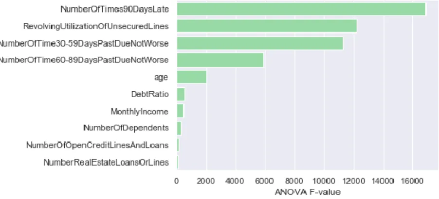
To measure feature importance, the ANOVA F-statistic was calculated. This metric can be used in classification problems, such as the one studied in this dissertation, to evaluate the relationship between the predictive features and the target variable. The calculation was achieved using the Scikit-learn feature selection function called f_classif (figure 4).

Figure 4 - Feature importance analysis (Kaggle dataset)

To assess the correlation between the predictive features, the Spearman's rank correlation coefficient was used (figure 5). This coefficient has an advantage in relation to Pearson’s correlation coefficient in the way it measures not only linear but also nonlinear relations between variables. In every pair of variables with Spearman’s rank correlation coefficient above 0.5, one of the variables was disregarded, more concretely, the one with lower ANOVA F-statistic value.

13

Figure 5 - Spearman’s correlation coefficient (Kaggle dataset)

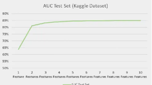
The two previous steps were complemented with a third analysis where the most important not strongly correlated variables were ordered and used to train a logistic regression model. That model was trained and tested in terms of performance (AUC metric) in several iterations (each iteration using a different number of features) to find the optimal number of features to be included in the models of each dataset. The cut-off point that was searched for in every dataset was the point where adding an additional variable to the logistic regression model had no longer significant gains in terms of performance measured on the test set (figure 6). The optimal number of features concerning each dataset is specified in table 5, and the final set of features included in the model is specified in table 6.

14

Figure 6 - AUC by number of features included in the model

Table 5 - Optimal number of features by dataset

Table 6 - Final set of features included in the models

3.4. A

This section gives a general overview of the algorithms used in this study, starting with the three single learning approaches (logistic regression, support vector machines and decision trees) and followed by the two ensemble learning approaches (random forest and stacking with cross-validation). This last algorithm (stacking with cross-validation) is the only technique that was not retrieved from the Scikit-learn library (it was retrieved from Mlxtend library). Some key parameters of these algorithms are also

Number of Features in the Original Dataset 10 15 20 14

Number of Features after One Hot Encode 10 28 50 26

Number of Features included in the models 6 7 8 4

Kaggle Dataset Japanese Dataset German Dataset Australian Dataset

Kaggle Dataset Japanese Dataset German Dataset Australian Dataset

1. NumberOfTimes90DaysLate 1. A9_t 1. A1_A14 1. A8_t

2. RevolvingUtilizationOfUnsecuredLines 2. A10_t 2. A1_A11 2. A10

3. NumberOfTime30-59DaysPastDueNotWorse 3. A8 3. A2 3. A7

4. NumberOfTime60-89DaysPastDueNotWorse 4. A6_R1 4. A6_A61 4. A5_R1

5. Age 5. A6_R5 5. A3_A34

6. DebtRatio 6. A7_R1 6. A3_A30

7. A4_u 7. A15_A152

15

discussed as they were tuned during the modelling process as described in the Modelling technique section of this dissertation.

3.4.1. Single classifiers

3.4.1.1. Logistic regression

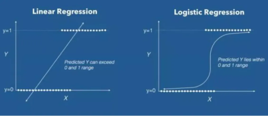
Logistic regression was developed by the statistician David Cox in 1958, and it consists of a parametric method that is widely used in the credit scoring models among financial institutions. The fact that logistic regression can be used to directly predict probabilities (Brid, 2018) is one of the main differences comparing to linear regression and it is quite useful when our dependent variable is categorical. In fact, linear regression has an output that can fall out of the range 0 to 1, being for that reason inappropriate for classification problems. Therefore, logistic regression is better suited for the particular context of credit scoring, given that we intend to predict the probability of a certain event to occur. Being more concrete, we want to predict the probability of a certain client to default (probability of our dependent variable being 1).

Figure 7 - Linear regression vs logistic regression

From: https://www.machinelearningplus.com/machine-learning/logistic-regression-tutorial-examples-r/ In logistic regression, a link function known as logit, the natural log of the odds, is used to establish a linear function with the input variables. In credit scoring context, with this link function that transforms our outcome variable, logistic regression manages to model a nonlinear association between the probability of default and the input variables in a linear way (formula 1). The logit function is also what enables to scale the independent variables to the scale of a probability (MacKenzie et al., 2018). In the same way linear regression uses the method of ordinary least squares to estimate the coefficients that provide the best fitting, logistic regression uses a technique called Maximum Likelihood Estimation that makes a guess for the values of the coefficients and iteratively changes them in order to maximize the log of the odds (Anderson, 2007). In other words, during the fitting process, this method will estimate the coefficients in such a way it will maximize the probability of being default of the individuals labelled as default as well as maximize the probability of not being default of the individuals labelled as non-default.

16

In the end, it results in a regression formula with the following form: ln( 𝑝(𝑑𝑒𝑓𝑎𝑢𝑙𝑡)

1 − 𝑝(𝑑𝑒𝑓𝑎𝑢𝑙𝑡)) = 𝛽0+ 𝛽1𝑥1+ 𝛽2𝑥2+ ⋯ + 𝛽𝑘𝑥𝑘+ ε

(1) where k is the number of independent variables.

That can be converted into a probability: 𝑝(𝑑𝑒𝑓𝑎𝑢𝑙𝑡|𝑋) = 𝑒

𝛽₀ + 𝛽₁𝑥1 + 𝛽₂𝑥2 +⋯+ 𝛽_𝑘𝑥𝑘

1 + 𝑒𝛽0 + 𝛽1𝑥1 + 𝛽2𝑥2 +⋯+ 𝛽𝑘𝑥𝑘

(2)

As logistic regression outcomes a probability, a cut-off probability or threshold needs to be fixed. As an example, if one fixes a threshold of 0.5 the model will classify every sample with a probability of default above 0.5 as positive (default) and every sample with a probability below 0.5 as negative (non-default).

In the past, there was a great disadvantage related to this model, which was its computational intensiveness, but with the progress in computer's capacities, this problem was overcome. That led to an increase in the popularity of this technique which is valued for being specifically designed to handle binary outcomes and for providing a robust estimate of the actual probability. Although logistic regression is still regarded as the industry standard technique (Lessmann et al., 2015), it is not free from several critics in literature that mainly reside in the assumptions it takes such as linearity between the independent variables and the log of the odds, or the absence of correlation among the predictors as well as the relevance of the predictors (Anderson, 2007). These assumptions are easily violated and naturally compromise the model's accuracy. The limited complexity associated with this technique is the main disadvantage in comparison to non-parametric more advanced machine learning techniques. Still, logistic regression has a strong advantage compared to other models which is the easy interpretation of its results. In fact, the coefficients associated to each independent variable that are estimated during the fitting process reveal, in a very direct way, the importance of each input variable as it expresses the size of their effect on the dependent variable.

The function available in Scikit-learn's library for using this model enables several parameters that can be tuned. Penalty is one of them, and it specifies the norm used in penalization. Another parameter used for model tuning is the C parameter that expresses, in an inverse way, the strength of the regularization.

3.4.1.2. Support vector machines

The interest in non-parametric techniques for credit scoring has been increasing. In opposition to parametric methods, they do not rely on many (or even any) assumptions about the data which release us from the risk of violating them during the modelling process and having losses of performance in our final predictive model. Machine learning and its increasingly obvious positive effects on business management have been supporting a renewed interest on relatively recent machine learning algorithms (Hue et al., 2017).

Support vector machines are strong machine learning models used in supervised learning both for classification and regression problems. The original form was firstly invented by Vladimir Vapnik and Alexey Chervonenkis in 1963 with the construction of a linear classifier. Later, (Boser, Guyon, & Vapnik,

17

1992), presented an SVM technique applicable to nonlinear classification functions such as polynomial and radial basis function stating good generalization when compared to other learning algorithms on optical character recognition problems. The approach followed by these authors consisted of applying the kernel trick to find the hyperplane that maximizes the margin. To understand how the support vector machines work, it is important for one to get familiar with the concept of margin. The margin is the distance between the decision line of the classifier and the closest observation. In the simplest scenarios, SVM models search for the maximal margin in the input space, which represents, with respect to binary classification problems, the largest buffer separating observations of the two different classes (Kirchner & Signorino, 2018). Depending on the number of predictive variables, the separating boundary can be a line if it has two predictive variables, a plane if it has three predictive variables or a hyperplane if it has four or more variables. The left panel of figure 8 (Kirchner & Signorino, 2018) exhibits an unrealistic scenario in terms of simplicity in which data is completely linearly separable. The input space has two predictive variables, 𝑋1 and 𝑋2, and the estimated plane H

separates successfully any observation with no misclassification errors. In fact, in a scenario such as the one presented on the left panel of figure 8 there is an infinite number of hyperplanes that are capable of separating the observations of the two classes, but one natural choice is the maximum margin classifier which consists of the separating hyperplane that is farthest from the training observations (James, Witten, Hastie, & Tibshirani, 2013). The especially signalled triangles and circles (open triangle and circles positioned throughout the margin) are named support vectors. These elements are the ones that determine the classifier, and so, if they were in a different position, the margin and the hyperplane position would not be the same anymore, and consequently, the classifier developed would be distinct. This logic is symbolic of the special way of functioning of support vector machines algorithms when compared to other machine learning methods in the way that it shows that the SVM models are more concerned on the observations of different classes that are more similar to each other (the ones closer to the margin) rather than focusing on the extreme examples of each class (the ones farther away of the margin). The right panel of figure 8 (Kirchner & Signorino, 2018) demonstrates a more realistic scenario where it is clear the pertinence of using the soft margin concept. It is not uncommon to find data that is not completely separable and so the idea of the soft margin is to allow some misclassification errors and to find a hyperplane that almost separates the two classes. The generalization of the maximum margin classifier to the non-separable data scenarios it is called support vector classifier (Haltuf, 2014). In this case, the support vectors are not only the vectors that lie directly on the margin but also the ones that lie on the incorrect side of the margin. The degree to which misclassification errors are allowed is defined in the C tuning parameter. The value for C is usually fixed via cross-validation, and the greater the C, the more tolerant the model will be with infringements to the margin, and by consequence the margin will also become larger. With that expansion, a bigger number of support vectors will be determining the hyperplane since there are more violations to the margin. In contrast, with a lower C, few support vectors will define the hyperplane, and one can expect a classifier with lower bias but higher variance as well (James et al., 2013).

18

Figure 8 - Linear SVM Classification (Kirchner & Signorino, 2018)

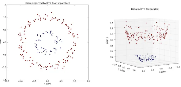
When one faces a nonlinear scenario like the one shown in figure 9, the support vector classifier will not be adequate to handle the classification problem. The target variable is not linear in relation to 𝑋1 and 𝑋2 predictive variables and, thus, no straight line can be drawn to separate the two classes

successfully without incurring in an unreasonable number of misclassifications. This is when support vector machines come in handy. Support vector machine is an extension of support vector classifier enlarging the feature space using the kernel tricks (James et al., 2013). This rationale is in line with the Cover's theorem which states that one can, with high probability, transform a non-linearly separable dataset into a linearly separable one projecting it into a space of higher dimension (figure 9). In a similar line of thought, a high dimensionality feature space is more likely to be linearly separable than a low dimension one, given that space is not densely populated (Cover, 1965). With the use of the nonlinear kernel functions the explicit calculation of the transformed vectors to achieve higher dimensionality is no longer needed and so the high computational effort associated with it is avoided. The kernel functions consist of measures of similarity between observations which correspond to the dot product of those observations in a higher-dimensional space, i.e. the dot product of the transformed vectors (P.Scheunders, D.Tuia, & G.Moser, 2018). In fact, the kernel functions take as input the observations in the original input space and return their similarity in the projected, higher dimensional, space. The kernel function also named simply kernels,

𝑘: 𝒳 × 𝒳 → ℝ (3)

can be defined as

𝑘(𝑥, 𝑥′) = ⟨𝜑 (𝑥) , 𝜑 (𝑥′_)⟩

𝑣 (4)

where ⟨· , ·⟩𝑣 is the dot product in the Hilbert space and 𝜑 the mapping function.

As a key restriction, ⟨· , ·⟩𝑣 must be a proper inner product. In fact, as long as 𝒱 consist of an inner

product space, the explicit representation of 𝜑 is not needed (P.Scheunders et al., 2018). With the kernel trick, a linear support vector classifier is found in the expanded space (right panel of Figure 10) and then it maps to a nonlinear classifier in the original space (S.Wilks, 2019). Figure 10, shows the result of a trained SVM with a nonlinear classification boundary, and the margin associated to it, in the

19

original data space (left panel) which has been obtained from the linear classifier visible in the right panel (S.Wilks, 2019). The kernel trick is not exclusive of support vector machines’ algorithms. In fact, any algorithm that depends solely on the dot product of the observations can integrate this adaptation (Haltuf, 2014).

Although there are several kernel functions, a popular one is the radial basis function which is represented by the following equation:

𝑘(𝑥, 𝑥′) = 𝑒𝑥𝑝 (−𝛾 ∥ 𝑥 − 𝑥′ _∥2_{) (5)}

Where ∥ 𝑥 − 𝑥′∥2 is the squared Euclidean distance between two samples represented in two feature vectors and 𝛾 is the inverse of the standard deviation of the radial basis function kernel. The gamma value (𝛾) of the radial kernel works as a parameter (for example, in the function of SVM classifier from Scikit-learn’s library) that defines the distance a single training observation can reach (Deepajothi & Selvarajan, 2013). Low values on the gamma parameter mean that a single training sample will have a wider influence. Another parameter of the radial basis function kernel is C. This latter expresses the balance between training examples misclassifications against decision surface simplicity (Deepajothi & Selvarajan, 2013). Contrary to what is stated by (James et al., 2013), and at least in the function of SVM classifier available in Scikit-learn’s library, low values on the C parameter will make the classifier more inclined to creating a smooth decision surface rather than classifying correctly every single training sample. This type of kernel searches for a support vector classifier in an infinite dimensionality space. This aspect of radial basis function makes this trick very flexible and able to fit a tremendous variety of decision boundary surfaces (Haltuf, 2014). Without the kernel trick, one would need to calculate the transformed vectors explicitly in the infinite-dimensional space, which would be impossible. Another characteristic of this kernel is its local behaviour, given that only nearby training observations have an effect on the class label of a new observation (James et al., 2013). Because of this characteristic, one can say that this type of kernel has a style of classification that is close to another machine learning algorithm, which is k-nearest neighbours.

Figure 9 - Projection of the original input space in a higher dimension space From https://towardsdatascience.com/understanding-the-kernel-trick-e0bc6112ef78

20

Figure 10 - Kernel Machine

From https://en.wikipedia.org/wiki/Support-vector_machine#/media/File:Kernel_Machine.svg

3.4.1.3. Decision tree

Although the concept of decision tree is not recent, decision tree algorithms have been gaining popularity with the growth of machine learning. This technique uses mathematical formulas like Gini index to find an attribute of the data, and also a threshold value of that attribute, in order to make splits of the input space (Patil & Sareen, 2016). In classification problems, those splits are performed in a way that best partitions the data in terms of discriminating individuals according to the class they belong to. Applied to the context of credit scoring, the algorithm will find the variables and the optimal split rules to end up, in each final bucket, with a group of individuals that are similar between them in terms of probability of default. In fact, besides the idea of grouping together individuals with similar probability of default, one wants at the same time to form groups that are different between them (Anderson, 2007). When it comes to understanding the splitting criterion, one must be familiar with the concepts of entropy and information gain. Entropy determines the impurity of a collection of individuals (Molala, 2019) in terms of their class. Moreover, it shows in which extent we are facing a group of individuals that is balanced in terms of the number of default and non-default (the two possible classes of our dependent variable). On the other hand, the concept of information gain refers to the expected reduction in entropy caused by partitioning the individuals using a given variable. Regarding entropy, as referred by (Akanbi, Oluwatobi Ayodeji Amiri, Iraj Sadegh Fazeldehkordi, 2015), there are two different concepts associated with the logic of operation of the algorithm.

▪ Target entropy: one uses all the data (or all the data in the parent node if the first split was already done) to count how many individuals there are in each class and consequently calculate the entropy

𝐸𝑛𝑡𝑟𝑜𝑝𝑦 (𝑆𝑒𝑡) = − ∑ 𝑃(𝑣𝑎𝑙𝑢𝑒𝑖 𝑘

𝑖=1

21

being K the number of classes of the dependent variable

▪ Feature’s entropy: for each feature, we calculate the expected child entropy, which is given by the entropies of the children weighted by the proportion of total examples of the parent node that are in each child.

𝐸𝑛𝑡𝑟𝑜𝑝𝑦 (𝐹𝑒𝑎𝑡𝑢𝑟𝑒 𝐴) = ∑ ( 𝑁º 𝑜𝑓 𝑖𝑛𝑠𝑡𝑎𝑛𝑐𝑒𝑠 𝑖𝑛 𝑐ℎ𝑖𝑙𝑑 𝑛𝑜𝑑𝑒 𝑖 𝑁º 𝑜𝑓 𝑖𝑛𝑠𝑡𝑎𝑛𝑐𝑒𝑠 𝑖𝑛 𝑡ℎ𝑒 𝑝𝑎𝑟𝑒𝑛𝑡 𝑛𝑜𝑑𝑒

𝑖∈𝑉𝑎𝑙𝑢𝑒𝑠(𝐴)

). 𝐸𝑛𝑡𝑟𝑜𝑝𝑦(𝑐ℎ𝑖𝑙𝑑 𝑛𝑜𝑑𝑒 𝑖) ₍₇₎

being A a given feature of the dataset and Values(A) the possible values of that feature. The information gain we get from splitting with the several feature options is assessed, and the feature that maximizes the information gain is the chosen one to do the split. The tree grows split after split and, in the end, in classification problems like credit scoring, it classifies the instances considering the most frequent class in each leaf. In case of regression problems, entropy indicator is not adequate to measure the impurity, so this is done calculating the weighted mean squared error of the children nodes. In the end, the predicted value of the target variable corresponds to the average of the true values of the samples in each node.

Decision trees result in models with low bias and are commonly associated with overfitting. That aspect is regarded as one of the major disadvantages of this technique. One popular way to control it is pruning the tree fixing a limit for its depth. In fact, trees with many levels and with terminal nodes that contain only a few numbers of samples is a typical overfitting scenario. On the other hand, there are advantages associated with decision trees models, for instance, the results easy to interpret and a clear capacity for modelling features that are not necessarily linear.

Concerning the parameters of this machine learning algorithm, Max_depth is a popular one that exists embedded in the model available in Scikit-learn library, and that represents the depth (or the number of levels) of the tree. As long one keeps increasing this parameter, one will get closer from a scenario where the classifier is able to classify all of the training data correctly. From a certain level onwards, it is better to stop since overfitting will certainly emerge. One can also use two parameters that control splitting by establishing minimum numbers of samples that have to be respected in order to perform more splits. Specifically, Min_Samples_Split expresses a minimum number of samples that an internal node needs to contain in order to do a new split whereas Min_Samples_Leaf is a minimum number of samples required to be at the leaf nodes or, also called, terminal nodes (Fraj, 2017).

3.4.2. Ensemble classifiers

One of decision trees models main disadvantages is that they are prone to overfitting due to its high variance and dependence on the training data. Although it is possible to control the decision tree fitting process in order to stop overfitting another valid alternative to avoid overfitting that exists in machine learning sphere, are the adoption of ensemble methods. Ensemble methods, in opposition to single learning approaches, train several base learners. This type of learning became popular in the 1990s, where two pioneering work were conducted. One, from Hansen and Salamon (1990), demonstrated that predictions resulting from a combination of several classifiers were more accurate than the ones performed by a single classifier. The other one, with Schapire (1990), demonstrated that weak learners (learners that perform just slightly better than random) could be turned into strong learners (Chapman, 2014).

22

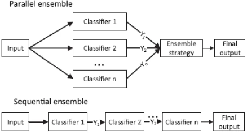
One way to segment the ensemble methods is according to the moment of generation of the several base learners. They can be generated in a sequential way, i.e. one after the other, or in a parallel process, i.e. the base learners are generated in parallel (Xia, Liu, Li, & Liu, 2017) (figure 11). The first segment is also called boosting, and these methods aim to lower bias and achieve a low generalization error. The second group of methods, also called bagging, tries to reduce variance but leaving at the same time bias unaffected (Vaishnavi, 2017).

Figure 11 - Parallel and sequential ensemble flux (Xia et al., 2017)

3.4.2.1. Random forest

Random forest is part of the second group, and it is a method capable of performing both classification and regression problems, that uses decision trees as base learners. It was introduced by Breiman in the early 2000s and became very popular since then. This approach relates to the concept of bagging, which implies the generation of different training sets for the various individual learners. In fact, the model is trained with samples drawn randomly with replacement (bootstrap samples) from the training dataset and using random feature selection in the process of each single tree generation (Brown & Mues, 2012). Therefore, in the case of having k trees (base learners), k samples are formed in a uniform way, collecting, with replacement, Z observations from the training set. The randomness associated with the way the training occurs in random forest algorithm contributes to the generated individual trees to be non-correlated between them.

Although random forests are used both for classification and regression problems, in the context of credit scoring it is used as an ensemble classifier. In case of classification, the algorithm chooses the class with the majority vote (figure 12) while in case of regression it averages the several outputs of the different models (Bhatia, Sharma, Burman, Hazari, & Hande, 2017). The underlying logic is that considering a set of individual learners to form a prediction gives more accurate results than relying on the prediction of a single learner. Random forest is seen as one of the most efficient machine learning algorithms since it is comparably insensitive to skewed distributions, outliers and missing values (Carvajal, Marko, & Cullick, 2018). Moreover, the predictive variables for random forest method can be of any type: numerical, categorical, continuous or discrete (Carvajal et al., 2018).

23

This machine learning algorithm has the same parameters options described earlier for decision tree algorithm, but it also has another popular one called N_estimators (Scikit-learn library’s terminology) that specifies the number of base learners being trained. Usually, the higher the number of estimators, the higher capacity of the model for learning with the training data (Fraj, 2017). Above a certain threshold that depends on the data and problem we are solving, there is no advantage in increasing this parameter as the computation effort will be much superior, and the performance on the test set can even decrease.

Figure 12 - Random forest

From https://www.datacamp.com/community/tutorials/random-forests-classifier-python#how

3.4.2.2. Stacking with cross-validation

Among the ensemble techniques, stacking is another type of approach. Literature has been more focused on homogeneous ensembles, and the stacking technique considered in this study consists of a heterogeneous ensemble learning approach. It was first implemented by (Wolpert, 1992) with the designation of Stacked Generalization where it was explained that the method works by deducing the biases of the base learners with respect to the training set. The deduction proceeds by building a (second-level) model that takes as inputs the outputs of the original base learners (first-level models). Base learners that are trained with a part of the training set and that make predictions, after the training, using the rest of the training set (Wolpert, 1992).

The Mlxtend library, Python library for machine learning tasks, firstly made available a stacking algorithm called StackingClassifier. This technique follows the generic spirit of stacking algorithms in the way it combines multiple classification models (first level classifiers) via a meta-classifier (second level classifier). Given a certain training dataset, all that data is used for training the base learners. Consequently, the outputs of those first models on the data used for training serve as features to the second level classifier fitting. As features for the second-level classifier can be used either probabilities or the predicted class (figure 13) (Raschka, 2014a). Stacking is a general framework in the way one can use single or ensemble learning approaches to generate first or second level classifiers. Compared with

24

other ensemble approaches such as bagging or boosting, stacking will work on discovering the optimal way of combining the base classifiers while the other two approaches will use voting (Aggarwal, 2014).

Figure 13 - Stacking classifier (Mlxtend library)

From http://rasbt.github.io/mlxtend/user_guide/classifier/StackingClassifier/

The Mlxtend library’s stacking algorithm presents the drawback of being prone to overfit. That is essentially because the features used in the second level model are derived from the same data that was used to train the first-level models (Aggarwal, 2014; Raschka, 2014a). To overcome this disadvantage, there is an alternative algorithm in the same Python Library (Mlxtend) called StackingCVClassifier. This alternative implements a similar logic but with the novelty of implementing the concept of cross-validation on the preparation of the input data for the second-level classifier. K-Fold is the applied cross-validation method, and it is also the most frequently used one to assess classification performance (Aggarwal, 2014; Raschka, 2014a).

The StackingCVClassifier algorithm (figure 14) starts by splitting the training dataset into k different folds. The number of k will dictate the number of iterations that will be performed. In each iteration, one-fold is left out while the others are used for training the first-level learners (our base learners) (Raschka, 2014b). Once those first-level learners are fitted, the algorithm uses those trained models to predict probabilities using as input the data contained in the previously left out fold (data that was not seen by the model while fitting). The process is repeated for each of k iterations, and the resulting probabilities are stacked and, in the end, used as input data to train our second-level learner (meta classifier) (Raschka, 2014b). After that, the algorithm repeats the first-level learners training process, this time using the whole training set. Applying the second level classifier on this updated first-level classifiers’ output, results in the final ensemble model output (Aggarwal, 2014).

The other four, previously described, classifiers of this study were used as first-level classifiers for the stacking algorithm. The previously tuned hyperparameters of those classifiers were considered in this

25

first-level classifiers' training. Logistic regression model was used as second-level classifier, and a new hyperparameter tuning was performed giving the fact that new data (first-level classifiers’ outputs instead of the original dataset features) was being inputted to this logistic regression model.

Figure 14 - Stacking with cross-validation classifier (Mlxtend library) From http://rasbt.github.io/mlxtend/user_guide/classifier/StackingCVClassifier/

3.5. M

3.5.1. Sample split

In order to control overfitting and evaluate the model’s capacity for generalization, it is necessary to keep a subset of the data out of the model training process. Only by doing that, one can be sure of the model effective performance and capacity for predicting accurately with new observations that were not “seen” during the training phase of the algorithm. As so, each of the four datasets used was randomly partitioned into two parts in a stratified way using Scikit-learn train_test_split function which means the proportion between default and non-default cases is equal in both training and test set. The percentage allocated for training was 70% while the remaining part was allocated for testing. Although there is not an explicit validation set, parameter tuning was performed using only the training set and through a five-fold cross-validation approach like the one illustrated in figure 15. More concretely, for every combination of hyperparameters, the model was trained five times (using in each time a different allocation of the training set between training and validation), and the performance was measured in those five iterations using the left-out fold destinated for validation in each iteration.