J. Braz. Comp. Soc. vol.12 número4

(1)

Brazilian Digital Television System

SBTVD

Luciano L. Mendes

1

_{, José Marcos C. Brito}

1

_{, Fabbryccio A. Cardoso}

2

_{, Dayan A. Guimarães}

1

Gustavo C. Lima3_{, Geraldo G. R. Gomes}1_{, Dalton S. Arantes}2_{and Richard D. Souza}4

1

Departamento de Telecomunicações Instituto Nacional de Telecomunicações

P.O. Box 05 Phone: +55 (35) 34719200

Zip 37540-000 - Sta. Rita Sapucaí - MG - BRAZIL {lucianol | brito | dayan | ge| }@inatel.br

2

Departamento de Comunicação Universidade Estadual de Campinas

P.O.Box 6101, Zip 13083-852 - Campinas - SP - BRAZIL {fabbryccio | dalton }@decom.fee.unicamp.br

3

Grupo de Pesquisa em Comunicação Universidade Federal de Florianópolis Campus Universitário, Florianópolis - SC - BRAZIL

guto@eel.ufsc.br Campus Universitário

4

CEFET/PR Curitiba - PR - BRAZIL richard@cpgei.cefetpr.br

Abstract

The objective of this paper is to present a general overview of the Innovative Modulation System Project -MI-SBTVD - developed for the Brazilian Digital TV Sys-tem. The MI-SBTVD Project includes an LDPC high per-formance error correcting code, an advanced transmit spatial diversity and an efficient multi-carrier modulation scheme. The building blocks of the system, its character-istics and most relevant innovations are presented. The performance of the whole system under different chan-nels is compared with the performance of the present-day Digital Television standards. The complete system was implemented in FPGA using VHDL language and rapid prototyping tools for DSP algorithms.

Keywords: Digital Television, LDPC Channel Cod-ing, OFDM Modulation, Spatial Diversity, SBTVD.

1. I

NTRODUCTION

(2)

all-digital proposal to implement an HDTV system. This proposal resulted in a recommendation by the ACATS (Advisory Committee on Advanced Television Systems) Special Panel in March 1993 that only a digital solution should be pursued [1].

The beginning of the standardization process started with the adoption in USA, in 1994, of the ATSC (Ad-vanced Television System Committee) standard. This standard has been developed by a group of companies called Grand Alliance. After that, the DVB-T (Dig-ital Video Broadcasting-Terrestrial) was developed and adopted in Europe and, finally, in 1999, the ISDB-T (In-tegrated Services Digital Broadcasting - Terrestrial) was adopted in Japan1_{. A brief description of each standard,}

including their main technical features, is given below.

1.1. ATSC

This standard does not support hierarchical transmis-sion, a feature supported by DVB and ISDB. The signal to noise ratio threshold for acceptable quality is around 15 dB in AWGN (Additive White Gaussian Noise) chan-nel, the best performance of the standards in this kind of channel. On the other hand, the performance of the re-ceiver under dynamic multipath channel is worst when compared with DVB and ISDB. The main characteristics of the ATSC standard, in terms of physical layer, are given in Table 1 [3].

Table 1. Main characteristics of the ATSC standard.

Characteristics

Modulation 8-VSB (Vestigial Side Band)

Inner Code TCM 2/3

Outer Code Reed Solomon (207, 187, 10)

Bandwidth 6 MHz

Total Symbol Rate 10.76 Mbauds Data Bit Rate 19.28 Mbps

1.2. DVB-T

This standard has been developed in Europe and it aims at fulfilling the requirements of all the European countries. Thus, the flexibility of the system has been an initial goal of the project.

The main difference between ATSC and DVB-T is in the number of carriers. While ATSC uses a single car-rier modulation, DVB-T adopted a multi-carcar-rier solution, using Coded Orthogonal Frequency Division Multiplex-ing (COFDM) with 2k or 8k carriers. The main reason for using this solution is the robustness of this scheme on frequency selective channels.

1_{It is important to observe that there are other standards in the world,}

like in China, but ATSC, DVB-T and ISDB-T are the most important ones.

Another advantage of the DVB-T, when compared with ATSC, is the hierarchical transmission of up to 2 data streams, which can be used for different applica-tions. This flexibility offers new business models for the TV broadcasters. For example, one option is to use one data stream to broadcast video and audio while the other one may transmit data associated with the scene. This implementation allows an interactivity of the user with the scene, opening new business opportunities. Another possible application is to use one data stream to broadcast SDTV (Standard Definition TV) while the other one is used to transmit the enhanced layer for the HDTV signal. Thus, the users that are capable to receive both streams can watch HDTV, while the users that can receive only the SDTV stream watch the program in standard defini-tion.

The main characteristic of the DVB-T standard, con-cerning the physical layer, are summarized in Table 2 [4].

Table 2. Main characteristics of the DVB-T standard.

Characteristics

Multiplexing COFDM

Modulation QPSK, 16-QAM or 64-QAM Inner Code Conv. 1/2, 2/3, 3/4, 5/6 or 7/8 Outer Code Reed Solomon (204, 188, 8)

Bandwidth 6 MHz, 7MHz or 8MHz Guard-time interval 1/4, 1/8, 1/16 or 1/32

Data Bit Rate 3.73 - 23.7 Mbps

1.3. ISDB-T

This standard has been based on DVB-T, what makes it so similar to the European standard. One advantage of ISDB-T over DVB-T is in an increased flexibility, sup-ported by a new concept for hierarchical transmission based on frequency segmentation. In this case, the total 6 MHz bandwidth channel is divided in 13 independent seg-ments that can be dynamically grouped to transmit up to 3 different data streams. Table 3 presents the main char-acteristics of ISDB-T [5].

Table 3. Main characteristics of the ISDB-T standard.

Characteristics

Multiplexing COFDM

Modulation DQPSK, QPSK,

16-QAM or 64-QAM Inner Code Conv. 1/2, 2/3, 3/4, 5/6 or 7/8 Outer Code Reed Solomon (204, 188, 8)

Bandwidth 6 MHz

Guard-time interval 1/4, 1/8, 1/16 or 1/32 Data Bit Rate / Seg. 0.28 - 1.79 Mbps

(3)

Televi-sion standards have been conceived in the 90’s of the last century. Since then, several important contributions have been proposed for the new generations of digital wireless communications systems. Thus, this is a great opportu-nity to propose a new standard for Digital Television that includes new technologies, resulting in a system with sig-nificant higher capacity and robustness when compared with today’s standards.

The goal of this paper is to present a proposal for the Brazilian Digital Television Standard using the state-of-the-art in communications technologies, offering signif-icantly improved performance when compared with the American, European and Japanese standards.

The remainder of this paper is organized as follows: Section 2 summarizes the main characteristics of the pro-posed standard; Section 3 presents the characteristics of a mobile channel for digital television. Section 4 shows the options considered and the decisions that have been made by the design team; Section 5 presents the performance of the system in different situations and also compares the MI-SBTVD with other digital television standards; Sec-tion 6 shows some implementaSec-tion issues and the solu-tions adopted to develop the prototypes. Finally, Section 7 presents the final conclusions.

2. MI-SBTVD

In the year 2005, the Brazilian government supported many research consortia in order to develop an advanced Digital Television System employing the most recent technologies for multimedia broadcasting. As part of this development, the MI-SBTVD (Innovative Modulation for the Brazilian Digital Television System) project has pro-posed a new solution for the physical layer of a new Dig-ital Television standard.

Some guidelines used in the MI-SBTVD project were:

• The SBTVD should have characteristics that facili-tate the integration of services, such as e-mail and multimedia services, in order to mitigate the "digital divide" social problem in Brazil.

• The system should have high digital capacity, allow-ing the transmission of HDTV or multiple programs in SDTV.

• The system should provide mobile reception using in-band transmission. Signals for fixed and mobile receptions should co-exist in the same 6 MHz band-width channel. This requirement is important to of-fer new business models for the broadcasters.

• The capacity and performance of the system should be better than of the former standards.

In order to achieve the goals defined above, the MI-SBTVD also uses a flexible hierarchical transmission based on frequency segmentation with 13 segments, as in the ISDB-T standard. Some important innovations in wireless communications technologies have been incor-porated in the MI-SBTVD project. For example, the inner code has been changed from a convolutional code (used in DVB-T and ISDB-T) to a Low-Density Parity-Check (LDPC) code. Besides, we have used a Space Time Cod-ing (STC) for transmit diversity. LDPC is a very efficient error correction code whose performance is very close to Shannon’s limit. Space Time Code is a technique pro-posed by Alamouti in 1998 that uses up to two transmit antennas and one or multiple receiving antennas to obtain space-time diversity. STC, associated with the OFDM, results in a very robust system for mobile reception on selective channels.

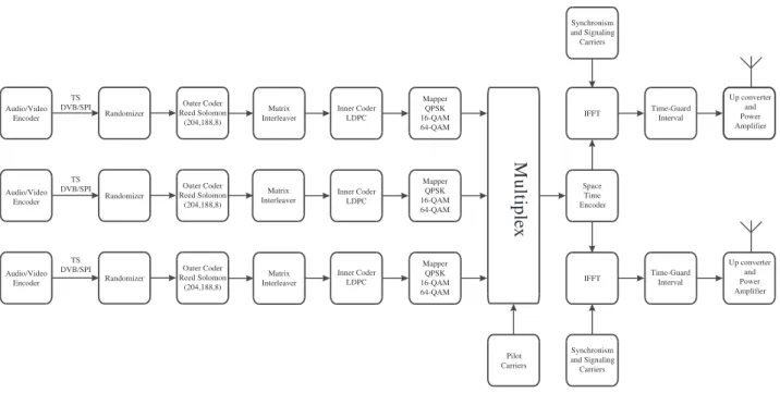
Figures 1 and 2 show the block diagram of the trans-mitter and of the receiver, respectively. The outer code is the same Reed Solomon (204,188,8) used in DVB-T and ISDB-T. The inner code is an LDPC with codeword length equal to 9792 and code rates 1/2, 2/3, 3/4, 5/6 and 7/8. The modulations are QPSK, 16-QAM and 64-QAM. This set of modulations allows the broadcasters to define the best trade-off between system throughput and robust-ness. The matrix interleaver between the inner and outer codes improves the performance of the RS decoder.

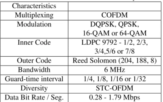
Table 4 summarizes the main characteristics of the MI-SBTVD system.

Table 4. Main characteristics of the MI-SBTVD system.

Characteristics

Multiplexing COFDM

Modulation DQPSK, QPSK,

16-QAM or 64-QAM Inner Code LDPC 9792 - 1/2, 2/3,

3/4,5/6 or 7/8 Outer Code Reed Solomon (204, 188, 8)

Bandwidth 6 MHz

Guard-time interval 1/4, 1/8, 1/16 or 1/32

Diversity STC-OFDM

Data Bit Rate / Seg. 0.28 - 1.79 Mbps

3. C

HANNEL

C

HARACTERIZATION

In this section the main characteristics of the wireless broadcasting DTV (Digital Television) channel are ad-dressed. These characteristics have been determinant in the design and testing phases of the MI-SBTVD system. Further details about them can be found in [6].

(4)

Inner Coder LDPC

Mapper QPSK 16-QAM 64-QAM

Inner Coder LDPC

M

u

lti

p

le

x

Space Time Encoder

IFFT

Time-Guard Interval

Pilot Carriers Randomizer

TS

DVB/SPI Outer Coder

Reed Solomon (204,188,8)

Randomizer TS

DVB/SPI Outer Coder

Randomizer TS

DVB/SPI Outer Coder

Matrix Interleaver

Matrix Interleaver Audio/Video

Encoder

Audio/Video Encoder

Synchronism and Signaling Carriers Synchronism and Signaling Carriers

Time-Guard Interval

Up converter and Power Amplifier Up converter

and Power Amplifier

Figure 1. Block diagram of the MI-SBTV transmitter for up to three hierarchical layers.

the overall system. The broadcasting DTV channel can be characterized as a multi-path fading channel in which time dispersion and frequency dispersion may vary with time, depending on the relative motion speed between the transmitter and the receiver. The time dispersion is mea-sured through the time delay profile of the channel and the frequency dispersion is measured through the Doppler profile of the channel.

The time delay profile varies according to the environ-ment. The mobility of the receiver is also important for the system specification, since the speed of the receiver determines the immunity that the system must have to the Doppler spread. Associated with these phenomena, the coherence bandwidth and the coherence time are the main parameters that must be analyzed.

The coherence time of the channel is the time inter-val in which the channel impulse response can be con-sidered approximately invariant. In other words, it is the time interval where the gain and the phase rotation in-troduced by the channel are highly correlated. Its value is inversely proportional to the Doppler spread, which is, in turn, directly proportional to the speed of the mobile receiver and the frequency of the signal. The coherence time does not depend on the channel impulse response. Knowledge about it was important to the development of the MI-SBTVD, since it determines the time-selectivity of the channel and, thus, restricts the choice of the mod-ulation to be adopted. It also has influence on the time-frequency interleaver design.

For illustration purposes, Table 5 presents the coher-ence time for different values of speed and frequency.

The Coherence Bandwidth of a channel is the band-width in which the channel frequency response may be considered approximately flat. In other words, it is the bandwidth where the correlation between the magnitude and phase of the channel is high, and it is independent of the speed of the mobile receiver. Knowledge about the co-herence bandwidth was important to the development of the MI-SBTVD, since it determines the frequency selec-tivity of the channel, which determines the spectral char-acteristics of the signal to be used by the system. It also has influence on the time-frequency interleaver design.

Table 6 shows the delay profiles for DTV static recep-tion and the corresponding coherence bandwidth of the channel [6]. The delay profiles in Table 6 are being used worldwide as reference for designing and testing DTV systems. The channel models Brazil A to Brazil E [7] represent the most common cases in Brazil.

A short description of each channel delay profile is presented as follows:

• UK short delay: describes reception conditions in cases where the terrain is flat.

• UK long delay: describes reception conditions in cases where the terrain has mountains.

(5)

Detector QPSK 16QAM 64QAM

D

e

m

u

lti

p

le

x

Time-guard Removal Space

Time Decoder

FFT Channel

Estimation

Tunner

Synchronism Recovery Transmission

Data Recovery Decoder

LDPC

Decoder LDPC

Decoder LDPC Audio/Video

Decoder Derandomizer

Derandomizer

Decoder Reed Solomon

(204,188,8)

Matrix

Deinterleaver

Matrix

Audio/Video Decoder

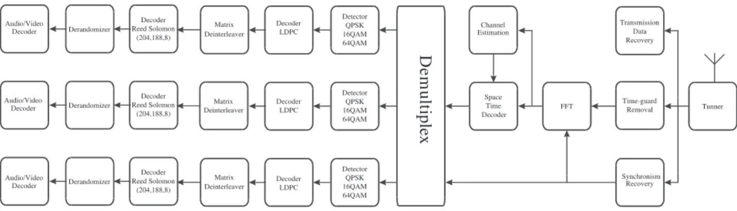
Figure 2. Block diagram of the MI-SBTV receiver for up to three hierarchical layers.

Table 5. Coherence time for different speeds and frequencies.

Freq / Speed 5km/h 30km/h 60km/h 80km/h 120km/h

54MHz 0.716 0.439 0.179 0.082 0.048

88MHz 0.119 0.073 0.03 0.014 7E-3

216MHz 0.06 0.037 0.015 6.8E-3 4E-3

470MHz 0.045 0.027 0.011 5.14E-3 3E-3

806MHz 0.03 0.018 7.46E-3 3.43E-3 2E-3

• CRC: this profile represents four different reception conditions that have been used to test ATSC equaliz-ers in Canada.

• Brazil-A: this profile simulates small echoes and short delays. It may represent a channel with line-of-sight in a flat terrain.

• Brazil-B: this profile represents a debilitated recep-tion with external antenna.

• Brazil-C: describes reception conditions in an envi-ronment with mountains and no line-of-sight.

• Brazil-D: represents reception conditions with inter-nal antenna.

• Brazil-E: describes reception conditions in a Single Frequency Network environment.

Another channel behavior that is particularly impor-tant to design the receiver of a DTV system is the im-pulsive noise. This kind of impairment is generated in a DTV channel and affects the received signal quality in two main ways: 1) impulsive noise generated by electric power circuitry or through direct induction in the receiver, and 2) impulsive noise captured by the receiver’s external antenna. Impulsive noise sources vary from oven igni-tion systems and fluorescent lamps switching to engine ignition systems. During the design and test of the MI-SBTVD, we identified impulsive noise types representing

worst-case receiver susceptibility for both internal and ex-ternal receptions.

Another important characteristic of the wireless broadcasting DTV channel, particularly relevant to the MI-SBTVD system design and testing, is the influence of the spatial correlation in the antenna diversity per-formance. As presented in Section 2, the MI-SBTVD adopted a transmit diversity technique in which the trans-mitted signal, after an appropriate processing, feeds two antennas. Then, two channels are established from the transmit antennas to the receiver antenna. The efficacy of this diversity scheme is better if the above-mentioned channels are uncorrelated or, at least, have low spatial cor-relation.

As illustrated in Figure 3, in a wireless broadcasting DTV channel with transmit diversity, the angle∆ϕthat embraces the electromagnetic waves capable of hitting the receiver antenna is directly proportional to the radiusain which the scatterers are distributed around the receiver. This angle is inversely proportional to the distanceb be-tween the transmitting base-station and the receiver. A typical value for∆ϕis 0.01 rd [6], ora/b= 0.005. This value is associated with the following scenario: radius of scatterersa= 15 m and distance between the base-station and the receiver,b= 3 km.

(6)

sig-Table 6. Channel delay profiles for Brazilian Digital Television Broadcasting.

Name Bc[kHz] Parameter Path 1 Path 2 Path 3 Path 4 Path 5 Path 6

Delay(µs) 0 0.05 0.4 1.45 2.3 2.8

UK Short Delay 18.41 Atten.(dB) 2.8 0 3.8 0.1 2.6 1.3

Phase 0◦ ₀◦ ₀◦ ₀◦ ₀◦ ₀◦

Delay (µs) 0 5 14 35 54 75

UK Long Delay 4.55 Atten. (dB) 0 9 22 25 27 28

Phase 0◦ ₀◦ ₀◦ ₀◦ ₀◦ ₀◦

Delay(µs) 0.5 1.95 3.25 2.75 0.45 0.85

DVB-T(Portable) 18.19 Atten.(dB) 0 0.1 0.6 1.3 1.4 1.9

Phase 336◦ ₉◦ ₁₇₅◦ ₁₂₇◦ ₃₄₀◦ ₃₆◦

Delay (µs) 0 -1.8 0.15 1.8 5.7 35

CRC Var1

Atten. (dB) 0 11 11 1 Var2 ₉

Phase 0◦ ₁₂₅◦ ₈₀◦ ₄₅◦ _Var1

90◦

Delay (µs) 0 0.15 2.22 3.05 5.86 5.93

Brazil A 13.75 Atten.(dB) 0 13.8 16.2 14.9 13.6 16.4

Phase 0◦ ₀◦ ₀◦ ₀◦ ₀◦ ₀◦

Delay (µs) 0 0.3 3.5 4.4 9.5 12.7

Brazil B 8.98 Atten.(dB) 0 12 4 7 15 22

Phase 0◦ ₀◦ ₀◦ ₀◦ ₀◦ ₀◦

Delay (µs) 0 0.089 0.419 1.506 2.322 2.799

Brazil C 18.43 Atten.(dB) 2,8 0 3.8 0.1 2.5 1.3

Phase 0◦ ₀◦ ₀◦ ₀◦ ₀◦ ₀◦

Delay (µs) 0.15 0.63 2.22 3.05 5.86 5.93

Brazil D 8.51 Atten.(dB) 0.1 3.8 2.6 1.3 0 2.8

Phase (Hz) 0◦ ₀◦ ₀◦ ₀◦ ₀◦ ₀◦

Delay (µs) 0 1 2 - -

-Brazil E 1.91 Atten. (dB) 0 0 0 - -

-Phase 0◦ ₀◦ ₀◦ _- _-

-1_{Variable according to the Communications Research Centre recommendation.}

Figure 3. Spatial diversity scenario.

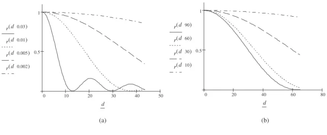
nal,d/λ, varyinga/band fixingξ. The angleξis related to the displacement of the receiver in relation to the line joining the transmit antennas (see Figure 3). Figure 4-b shows the spatial correlation ρr as a function of d/λ,

varyingξand fixinga/b.

It can be seen from Figure 4-a that the spatial corre-lationρris strongly dependent on the ratio between the radius of scatterers,a, and the distance between the base-station and the receiver,b. Poor scattering environments (smalla) and high distancebtend to increase the spatial correlation between the signals transmitted from the two antennas to the receiving antenna. Observing Figure 4-b, we can see that the spatial correlationρris also strongly dependent on the angleξdefined in Figure 3. Receivers located in front of the base-station transmit antennas tend to benefit from lower correlations than receivers located in positions with smallξ. The vertical displacement of the transmitting antennas can solve this problem, since

ξwill remain practically constant and around 90o_{. This}

(7)

0 10 20 30 40 50 0.5

1

r d( 0.03)

r d( 0.01)

r d( 0.005)

r d( 0.002)

d

0 20 40 60 80

0.5 1

r d( 90)

r d( 60)

r d( 30)

r d( 10)

d

(a) (b)

Figure 4. Spatial correlationρras a function ofd/λ. Varyinga/bandξ= 90o(a). Varyingξanda/b= 0.006 (b).

is in a better situation for coverage. This will demand the use of different transmitting powers in each antenna. The effect of different transmitting powers in the overall system performance should be carefully analyzed.

3.1. PERFORMANCE OF THE MI-SBTVD UNDER

IMPULSIVE NOISE

As briefly mentioned in this Section, for testing the MI-SBTVD we identified impulsive noise types repre-senting worst-case receiver susceptibility for both internal and external reception The impulsive noise impairments were generated according to the model depicted in Figure 5 and the parameters given in Table 7, where∆Smin is the minimum space between pulses inµs,∆Smax is the maximum space between pulses inµs andSef f ect is the effective duration inµs. Further details can be found in [6].

Burst duration Pulse duration (250 ns)

Effective burst duration Burst spacing (10 ms)

Figure 5. Impulsive noise model.

The results concerning the MI-SBTVD impulsive noise immunity, presented in Section V, are interpreted according to Figure 6. In this figure there are five regions,

Table 7. Parameters for Impulsive Noise Testing.

Test Pulse / burst ∆Smin* ∆Smax* Sef f ec

A 1 N/A N/A 0.25

B 2 1.5 45 0.5

C 40 0.5 1 10

* Within a burst, the space between pulses are uniformly distributed between the minimum and maximum values specified.

which are described below:

• This asymptotic behavior occurs when the ratio be-tween the signal power and the impulsive noise power (C/I) tends to infinity. It reveals the system performance under AWGN when it reaches the TOV (threshold of visibility).

• When the ratio between the signal power and the AWGN power (C/N) tends to infinity we get the min-imumC/Inecessary for the system to reach the TOV.

• This intermediate region reveals the system perfor-mance under the combined effect of the AWGN and impulsive noise.

• A shift in this curve to the left reveals greater im-pulsive noise immunity, in terms ofC/I. The lower bound on this shift corresponds to the value in dB depicted by the number 5 in the figure.

(8)

Figure 6. Curves for the MI-SBTVD performance evaluation under AWGN and impulsive noise.

4. S

YSTEM

D

ESIGN

The main objective of the system proposed in the pre-vious section is to obtain higher performance when com-pared with the Broadcasting DTV standards available to-day. Besides the performance improvement, the system also needs to guarantee a good trade-off solution between robustness and data rate. This flexibility is important because it allows the TV operators to choose between large coverage with SDTV signal or small coverage with HDTV signal, for example. The next subsections describe each block that composes the system.

4.1. RANDOMIZER

The audio and video information, compressed and multiplexed by the audio and video encoders at the MPEG layer, are represented by a bit stream. The Transport Stream (TS) is defined by the MPEG standard as an alter-native to transmit the encoded information. In this case, the encoded data is organized in packets of 188 bytes, where the data rate is kept constant by adding null-packets [8]. Figure 7 presents the structure of the TS. The most important information in the TS header for the physical layer is the Synchronism Byte that is47H.

The TS may have a long sequence with certain pe-riodicity, depending on the scene that is being encoded. This periodicity results in spectral concentration, which reduces the performance of the system in selective fad-ing channels, and also may cause synchronism problems at the receiver. In order to avoid the problems associated with long cyclic sequences, the encoded data is multiplied by apseudo-noise (PN) sequence generated through the polynomial

g(x) = 1 +X14

+X15

(1)

The initial seed of the generator isA9H, and it must be

re-initialized at the beginning of each new OFDM frame.

4.2. CHANNELCODE

Among the well-know coding channel techniques, a preliminary research suggested the BICM (Bit-Interleaved Coded-Modulation) as a suitable technique for the SBTVD channel models. The BICM gives best performance on fading channels compared to conven-tional coded modulations. However, the same does not happens for the AWGN channel, where coded modula-tions like TCM (Trellis Coded Modulation) gives better results than BICM [9]. BICM was also considered with iterative decoding, or BICM-ID (Bit-Interleaved Coded Modulation with Iterative Decoding), in order to improve the BICM performance on AWGN channels.

In fact, BICM can be interpreted as any coding scheme in which the coded bits are interleaved prior to symbol mapping and modulation. Euclidian distances are not explored as done in conventional coded modulation techniques. The complexity of BICM-ID implementation representes an additional obstacle to the system develop-ment in the project schedule. Then, the design team has decided to search for powerful channel coding schemes that could show good performance for both the AWGN and the fading channels. This decision led the team to the capacity-achieving Turbo [10] and LDPC (Low-Density Parity-Check) [11] codes.

The original Turbo codes [10] correspond to the par-allel concatenation of recursive and systematic convolu-tional codes, with a symbol-by-symbol MAP (maximum a posteriori) iterative decoding algorithm. Nowadays, the term Turbo codes has a more generic meaning. Turbo coding is any channel coding technique that uses: 1) an iterative decoding process and 2) a concatenation of in-terleaved component codes.

Basically, there are two Turbo codes families: the first one is based on a concatenation of convolutional code (CTC, Convolutional Turbo Codes) and the second one is based on a concatenation of block codes (BTC, Block Turbo Codes). Among the BTCs, Single-Parity Check Turbo Product Codes (SPC-TPC) were investigated. The aim of this choice was a reduction in complexity, a fast decoding and, possibly, some performance improvement as compared to high-rate and short convolutional Turbo codes [10].

LDPC codes belong to the class of linear block codes. Their name is due to the parity-check matrix intrinsic characteristic of having a low number of ones, as com-pared to the number of zeros. The main attribute of LDPC codes is that their performance is also near to the capacity of several communication channels. Besides, the LDPC decoding may be implemented with parallel architecture and relatively low complexity algorithms, as compared to most of the Turbo decoding algorithms [12].

(9)

Rate Adaptation or Payload

H

188 bytes

Sync. Byte

Transport error indication

Start indication

Transport priority

Program identification

Scrambling Rate adaptation

control

Continuity counter

4 bytes

Field adaptation control

Figure 7. Data structure of the MPEG Transport Stream.

Turbo Codes assembled with Single-Parity Check Prod-uct Codes and irregular LDPC codes. These comparisons were carried out by means of computer simulations on AWGN and flat Rayleigh fading channels. The results obtained showed that the LDPC codes produce better per-formance compared to Turbo codes when the BER (Bit Error Rate) is above the LDPC error floor. The choice in favor of the LDPC code was made based on the reasons: better performance than the SPC-TPC codes; great design flexibility and not too big decoding complexity. Besides, LDPC codes require almost no royalties to be paid, as compared to Turbo codes.

The LDPC error floor can be reduced by the concate-nation of the LDPC with some other outer coding scheme. The Reed-Solomon (RS) channel coding was the choice, since it is efficient and can be decoded with low complex-ity.

With the code already defined, the next step was the choice of the LDPC length suitable to the SBTVD seg-mentation. The segmentation adopted by the SBTVD OFDM (Orthogonal Frequency-Division Multiplexing) was the same as the one adopted by the ISDB-T system (ARIB STD-B31 V1.5) [5]. This choice was justified by the fact that the project schedule did not allow us to eval-uate the impact of a new segmentation on the system im-plementation and performance. The combination of the ARIB STD-B31 V1.5 segmentation, the OFDM frame structure and the RS (204, 188) was determinant on the possible LDPC lengths. Besides, different LDPC cod-ing rates were considered in order to optimize the perfor-mance with regards to the segmentation and the channel models. The coding rates 1/2, 2/3, 3/4, 5/6 e 7/8 were de-fined. The LDPC lengths and the average error correction capability for a 1/2 coding rate are shown in Table 8.

Initially, the LDPC with code length 39168 was in-vestigated as a possible and efficient solution to eliminate the channel interleaver and, consequently, to simplify the hardware. In fact, computer simulations on the SBTVD channels, including impulsive noise impairments, indeed

Table 8. LDPC lengths and their error correction capability for coding rate R = 1/2

Lenghtn(bits) Average error correctiont(bits)

39168 5162

19584 2520

13056 1645

9792 1211

6528 787

4896 573

2304 241

showed that the channel interleaver was not necessary [12]. However, the external code RS (204, 188) cascaded with then= 39168 LDPC did not reduce the error floor as expected. This was caused because the LDPC residual errors exhibited frequent burst patterns, exceeding the RS error correction capability.

The trade-off solution between the interleaver elimi-nation and the error-floor reduction was the adoption of the classic solution: an interleaver between the RS (204, 188) and the LDPC encoders. However, to avoid a long delay in the decoding process, an LDPC withn= 9792 was chosen. Since the interleaver length depends on the modulation, different lengths were adopted, according to Table 9.

Table 9. Possible interleaver lengths depending on the modulation.

Modulation Interleaver Length

QPSK 4 LDPC words

16-QAM 8 LDPC words 64-QAM 12 LDPC words

(10)

same reasoning can be applied to 16- and 64-QAM mod-ulations.

The number of data bytes necessary to compose a LDPC word depends on the code rate used. Table 10 shows the number of data bits and data bytes necessary to form an LDPC word.

Table 10. Number of data bits or byte to compose a LDPC word depending on the code rate.

Code Rate Number of Bits and Bytes

1/2 4896 bits or 612 bytes 2/3 6528 bits or 816 bytes 3/4 7344 bits or 918 bytes 5/6 8160 bits or 1020 bytes 7/8 8568 bits or 1071 bytes

4.3. TRANSMIT DIVERSITY USING SPACE-TIME

CODING

Television broadcasters are very interested in expand-ing their business model to mobile television, especially for cellular reception. Therefore, the Digital Television system must provide robustness for mobile reception, so the impact of the Doppler spread on the system perfor-mance must be minimized. Receivers with spacial diver-sity [13] could be a solution to this problem. Neverthe-less, for a digital television broadcasting system, to keep costs and complexities only in the transmitter, it is more interesting to provide transmit diversity instead of recep-tion diversity, since only the transmitter may have multi-ple antennas.

In 1998, Alamouti proposed a transmit diversity tech-nique using space-time coding [14]. In this scheme, two transmitting antennas andLreceiver antennas can be used to obtain a diversity gain of order2L. However, the com-munication channel must be characterized by flat, non-selective fading. It is also assumed that the coherence time of the channel is greater than the duration of two consecutive modulation symbols. Moreover, the receiver must perfectly know the channel in order to obtain full diversity gain. However, high transmission rates asso-ciated with the mobility of the receivers result in a fre-quency selective, time-variant fading channel. The condi-tions above are sufficient to guarantee transmit diversity when the Alamouti scheme is associated with the OFDM technique.

4.3.1. OFDM: Digital data broadcasting channels

usually present multiple paths between the transmitting and the receiving antennas [15]. In this scenario, high data rate signals suffer from frequency selective fading.

The basic principle of OFDM transmission technique is to divide the high rate stream intoNlower rate streams.

This procedure may transform the original selective fad-ing channel into several flat fadfad-ing channels. Each lower symbol rate stream is transmitted using a different sub-carrier. In order to maximize the spectral efficiency, the sub-carriers are mutually orthogonal. The orthogonality is achieved when the frequency separation between two adjacent sub-carriers is equal to the symbol rate of each sub-stream.

The OFDM symbol can be generated using the Inverse Fast Fourier Transform (IFFT). The sampled version of the OFDM symbol is given by [16]

sm= N₋1

X

k=0

ckexp

j2πk

N m

(2)

whereck=ik+jqkis the vector of complex data symbols andm= 0,1,2, . . . , N −1is the discrete sample time of the OFDM signal.

Using Eq. (2) it is possible to generate OFDM signals by using computational methods, avoiding the synchro-nism problems with oscillators. Figure 8 shows the block diagram of an OFDM system.

A guard-time interval is used to increase the robust-ness of the system. The MI-SBTVD system employs a cyclic prefix that is formed by part of the the OFDM sym-bol which is copied to its beginning, as can be seen in Figure 9.

t

s

(

t

)

Figure 9. Guard time interval for OFDM symbols.

In the MI-SBTVD system, it is possible to define a cyclic prefix of 1/4, 1/8, 1/16 or 1/32 of the OFDM sym-bol time as a guard-time interval.

4.3.2. Transmit Diversity: Space-Time Block Code

(11)

Bits

Modulador

Digital ck=ik+jqk Serial/Parallel

Converter c₀ i0+jq0 c1

i1+jq1

. . . . . . cN-1

i_N-1+jq_N-1

IFFT

NSamples FFT .._.

c'0

c'1

c'_N-1

N samples Channel 0 . . . i'+jq'0

i'1+jq'1

i'_N-1+jq'_N-1

Detector Bits Parallel/Serial

Converter c'_L

Figure 8. Block diagram of an OFDM system.

STBC uses the transmission matrix given by

Ant1 Ant2

ti ci −c∗i+1

ti+1 ci+1 c∗i

(3)

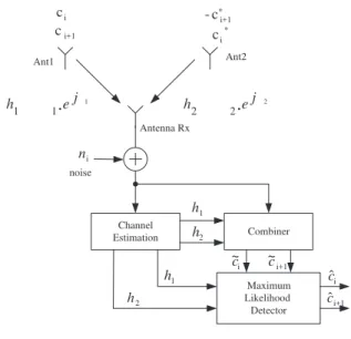
This transmission matrix combines the signals trans-mitted by both antennas, increasing the performance of the system in flat, time-variant channels. Figure 10 shows the block diagram of this system.

Ant1 1

.

1 1 j e

h

.

2

2 2 j e h * i c i n noise Ant2 Antenna Rx Channel Estimation Combiner 1 h 2 h Maximum Likelihood Detector 1 h 2 h i ~

c ~ci+1

i ˆ c i+1 ˆ c i c * i+1 c -i+1 c

Figure 10. Block diagram of the STC system.

Symbols transmitted by Antenna 1 suffer an attenua-tion and phase rotaattenua-tion given by

h1=α1ejθ1 (4)

while symbols transmitted by Antenna 2 suffer an attenu-ation and phase rotattenu-ation given by

h2=α2ejθ2 (5)

whereα1andα2are assumed to be independent random

variables with Rayleigh distribution andθ1andθ2are

as-sumed to be independent random variables with uniform distribution between−πandπ[13]. These random vari-ables are assumed to be constant over two symbol inter-vals.

The signals at the input of the receiver in the time in-stanttiandti+1are respectively given by

ri=h1ci−h2c∗i+1+ni ri+1=h1ci+1+h2c∗i +ni+1

(6)

whereniandni+1are the AWGN noise samples at time

instantstiandti+1, respectively. In order to obtain full

di-versity gain, the detector must have perfect knowledge of the channel parameters. The channel estimation block is responsible for providing these parameters. The combiner uses this information to obtain the diversity provided by the space-time coding, combining the signals as follows:

ˆ

ci=rih∗1+r∗i+1h2

= α2

1+α

2 2

ci+nih∗1+n∗i+1h2 ˆ

ci+1=h∗1ri+1−h2ri∗

= α2

1+α

2 2

ci+1−n∗ih2+ni+1h∗1

(7)

The performance of the Alamouti scheme is equiva-lent to the performance of the Maximum Ratio Combiner (MRC), except for a penalty of 3 dB due to the power division in the two transmitting antennas and the double noise addition.

4.3.3. Space-Time Coding and OFDM: There are

two different ways to associate the Alamouti scheme with the OFDM transmission technique. The first one uses two OFDM symbols to build the space-time transmission matrix, resulting in a space-time block coding OFDM (STBC-OFDM) scheme [20]. Figure 11 shows the block diagram of this system.

The transmission matrix is given by

Ant1 Ant2

kth_{carrier of}_ith_{OFDM symbol} _c

i −c∗i+1

kth_{carrier of}₍_i_{+ 1)}th_{OFDM symbol} _c

(12)

Ant. 1

Ant. 2

h1(f)

h2(f)

IFFT

Receiver t=iT

t=(i+1)T

. . . . . . sub-carrier 1 . . . c1 c3 c5 c7 c9 c11 c13

-c2*

-c4*

-c6*

-c8*

-c10*

-c12*

-c*14

. . . c2 c4 c6 c8 c10 c12 c14 . . .

c1* c3*

c5* c7*

c9* c11*

c13*

. . . sub-carrier 2 sub-carrier 3 sub-carrier 4 sub-carrier 1 sub-carrier 2 sub-carrier 3 sub-carrier 4

Figure 11. Block diagram of the STBC-OFDM system.

channels that have small coherence bandwidth and large coherence time [17].

The receiver must know the channel frequency re-sponse in order to obtain full diversity gain. Pilot sub-carriers are introduced in the OFDM symbol to help es-timation of the channel frequency response. Figure 12 shows pilot sub-carriers in an STBC-OFDM system.

Ant. 1

Ant. 2

h1(f)

h2(f)

IFFT

Receiver t=iT

t=(i+1)T

. . . . . . sub-carrier 1 . . . p1 c1 c3 p3 c5 c7 p5

-p2*

-c2*

-c4*

-p4*

-c6*

-c8*

-p6*

. . . p2 c2 c4 p4 c6 c8 p6 . . .

p1* c1*

c3* p3*

c5* c7*

p5*

. . . sub-carrier 2 sub-carrier 3 sub-carrier 4 sub-carrier 1 sub-carrier 2 sub-carrier 3 sub-carrier 4 Legend ci => Data symbol.

pi=> Pilot symbol

Figure 12. Pilots sub-carriers in an STBC-OFDM system.

The pilot symbols,pi, are known to the receiver. Thus, it is possible to estimate the channel frequency response for the pilot sub-carriers. For high sinal-to-noise ratios, the received signals at theith

pilot sub-carrier frequency,

fi, are given by

rk=pkh1(fi)−p∗k+1h2(fi) rk+1=pk+1h1(fi) +p∗kh2(fi)

(9)

Assuming thatpk =pk+1=pandp∈ ℜ, solving (9) for

h1(fi)andh2(fi)results in

h1(fi) =

rk+1+rk

2p

h2(fi) =

rk+1−rk

2p

(10)

In order to obtain an estimation of the frequency response for all frequencies, it is necessary to interpolate the esti-mation obtained in (10). There are several different inter-polation techniques that can be used to obtain an estima-tion of the channel frequency response at the frequencies of the data sub-carriers [18].

The second alternative to combine space-time cod-ing with the OFDM transmission technique is to use two adjacent sub-carriers to build the space-frequency trans-mission matrix, which results in a space-frequency block coding OFDM (SFBC-OFDM) scheme [21]. Figure 13 presents the block diagram of this system.

Ant. 1

Ant. 2

h1(f )

h2(f ) IFFT IFFT ... ... Receiver c1 c3 c1* c3* sub-carrier 1 sub-carrier 2 sub-carrier 3 sub-carrier 4 sub-carrier 1 sub-carrier 2 sub-carrier 3 sub-carrier 4 c2 -c 2* c4 * -c 4

Figure 13. Block diagram of the SFBC-OFDM system.

The transmission matrix is given by

Ant1 Ant2

ith

carrier ofkth

OFDM symbol ci −c∗i+1 (i+ 1)th

carrier ofkth

OFDM symbol ci+1 c∗i (11) Again, Eq. (7) can be used to obtain the diversity gain from the received signals, whererjis the received signal on thejth _{sub-carrier at the same OFDM symbol. The}

channel frequency response must be the same for two ad-jacent sub-carriers and time-invariant during one OFDM symbol interval.

It is also possible to use pilot carriers and linear in-terpolation to estimate the channel frequency response. Here, two adjacent pilot sub-carriers are used to estimate the channel frequency response that must be the same for both sub-carriers.

The received signals at the frequencies of the pilot sub-carriersfiandfi+1are given by

ri=pih1(fi)−p∗i+1h2(fi) ri+1=pi+1h1(fi+1) +p∗ih2(fi+1)

(13)

whereh1(fi)is equal toh1(fi+1),pi = pi+1 =p ∈ ℜ

and then (10) is used to obtain an estimation of the chan-nel frequency response on the frequencies of the pilot sub-carriers. The estimation of the channel frequency re-sponse at the frequencies of the data sub-carriers can be obtained by using an interpolation algorithm.

Both schemes (STBC-OFDM and SFBC-OFDM) pre-sented here have advantages and disadvantages, which are related to the correlation among these sub-channels. Doppler spread and frequency response of the channel define which scheme should be used. In order to define which scheme is suitable for a DTV Standard, the perfor-mance of both approaches were compared for the chan-nels presented in Table 6.

The mobility of the receiver is simulated by multiply-ing each path of the channel by a random variable with Rayleigh distribution and mean square valueσ2

r = 1. The phase of each path is added to a random variable uni-formly distributed between−πandπ. Two speeds have been considered: 60km/h for channel 13 (216MHz) and 120km/h for channel 69 (806MHz). The mobility of the receiver results in a time-variant channel. The space-time or space-frequency decoders require that the channel must be constant over the duration of a codeword. It means that the channel must be time-invariant for one OFDM sym-bol duration for an SFBC-OFDM. For STBC-OFDM, the channel must be time-invariant during at least two OFDM symbol intervals.

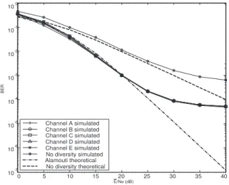
Table 11 presents the system parameters used in the simulations and Figure 14 presents the performance of the STBC-OFDM for a receiver moving at 60 km/h and chan-nel 13, which results in a Doppler spread of 12 Hz. Figure 15 presents the performance of the SFBC-OFDM for the same conditions.

Table 11. System parameters.

Parameters Value

Data Modulation QPSK

Total Number of sub-carriers 2048 Sub-carrier spacing 3.97 kHz

Pilot modulation BPSK

Guard-time interval T/16

Total OFDM symbol duration 267.5µs

Equalization Perfect estimation

Comparing Figures 14 and 15 it is possible to con-clude that the STBC-OFDM scheme is better than the SFBC-OFDM scheme in all channels. The performance of SFBC-OFDM is highly penalized when the coherence bandwidth of the channel is reduced. The reduction of the coherence bandwidth does not severely affect the STBC-OFDM scheme because this scheme does not require the same frequency response for two adjacent sub-carries, as

E/No (dB)

0 5 10 15 20 25 30 35 40

10-7

10-6

10-5

10-4

10-3

10-2

10-1

100

B

E

R

Channel A simulated Channel B simulated Channel C simulated Channel D simulated Channel E simulated No diversity simulated Alamouti theoretical No diversity theoretical

Figure 14. Performance of STBC-OFDM system with Doppler spread of 12Hz.

the SFBC-OFDM does.

Figure 16 presents the performance of the STBC-OFDM for a receiver moving at 120 km/h and channel 69, which results in a Doppler spread of 89 Hz. Figure 17 presents the performance of the SFBC-OFDM for the same conditions.

Comparing Figures 16 and 17 it is possible to con-clude that the SFBC-OFDM is better than SFBC-OFDM when the mobility of the receiver is high. These behav-iors are related to the fact that the frequency selectivity of the channels plays a minor role in the performance of the schemes, while the Doppler spread plays a major role. The fact that SFBC-OFDM requires a lower channel co-herence time than STBC-OFDM results in its better per-formance.

The MI-SBTVD design team has decided to use STBC-OFDM, because the most common scenario for DTV reception is with a small Doppler spread. The simu-lation results presented in this paper show that the perfor-mance of the STBC-OFDM in this case is better than the performance of the SFBC-OFDM for all channel profiles.

4.4. OFDM FRAMESTRUCTURE

The structure of the OFDM frame is based on the ISDB-T standard. There are three available modes: Mode 1, employing a 2048-point FFT, Mode 2 with 4096-point FFT and Mode 3 with 8192-point FFT. The first mode is robust to Doppler spread but it is not suitable for Single Frequency Network (SFN) [19]. Mode 3 is suitable for SFN, but it is not robust to Doppler spread. Mode 2 is an intermediate solution that can be used in low-speed mo-bile reception in an SFN.

(14)

0 5 10 15 20 25 30 35 40

10-7

10-6

10-5

10-4

10-3

10-2

10-1

100

E/No (dB)

B

E

R

Figure 15. Performance of SFBC-OFDM system with Doppler spread of 12Hz.

length. These segments can be freely grouped to transmit up to three different data streams (layers). A segment is composed by data carriers, scattered pilots carriers (SP), transmission and multiplexing configuration and control carriers (TMCC). There are also auxiliary carriers (AC) that can be used as complementary signaling. MI-SBTVD uses these carriers to identify the first OFDM symbol of the Space Time Code. Table 12 shows the composition of a segment based on the FFT length.

Table 12. Number of carriers per segment.

Mode 1 Mode 2 Mode 3 2048 FFT 4096 FFT 8192 FFT

Total 108 216 432

Data 96 192 384

SP 8 18 36

TMCC 1 2 4

AC 2 4 8

The OFDM frame is composed by 204 OFDM sym-bols. This number guarantees an integer number of Reed Solomon codewords, regardless the code rate, guard time interval, modulation order, segment combination or FFT length. The number of LDPC codewords is a multi-ple of 0.5, which means that it may be necessary two OFDM frames to obtain the LDPC synchronism. Table 13 presents the number of codewords per segment, as a function of the modulation order and FFT length.

5. P

ERFORMANCE

A

NALYSIS

In this section we present performance results of the modulation and channel coding schemes developed for

E/No (dB)

0 5 10 15 20 25 30 35 40

10-7

10-6

10-5

10-4

10-3

10-2

10-1

100

B

E

R

Figure 16. Performance of STBC-OFDM system with Doppler spread of 89Hz.

Table 13. Number of codewords per segment.

Mode Modulation LDPC R&S

QPSK 4.5 216

Mode 1 16QAM 9 432

64QAM 13.5 648

QPSK 9 432

Mode 2 16QAM 18 864

64QAM 27 1296

QPSK 18 864

Mode 3 16QAM 36 1728

64QAM 54 2592

the MI-SBTVD system. All the results have been ob-tained by computer simulation, using Matlab Simulink. The results presented here are a subset of the results re-ported to the Brazilian Communications Ministry [22].

As described in Section 3, ITU suggests some typi-cal channel profiles that can be used to test DTV systems with fixed reception (Brazil A, B, C, D and E) and mo-bile reception (Typical Urban GSM). The performance of the system has been tested for all of these channels, for AWGN channel with and without impulsive noise.

The following general specifications have been con-sidered in the simulations:

• Channel Coding: in the final specification of the sys-tem the internal code is a LDPC with block length equal to 9 kbits. In our preliminary tests, we have used LDPC with block length equal to 9 kbits or 39 kbits. The results reported here, when not specified, correspond to LDPC block length equal to 39 kbits.

(15)

E/No (dB)

0 5 10 15 20 25 30 35 40

10-7

10-6

10-5

10-4

10-3

10-2

10-1

100

B

E

R

Figure 17. Performance of SFBC-OFDM system with Doppler spread of 89Hz.

• Guard Time: the guard time was fixed at 1/16 of the OFDM symbol period in all the simulations.

• Channel Estimation and Synchronization: perfect channel knowledge and synchronism are assumed. This choice has been made in order to evaluate the system potential, without regarding to the limitations of one receiver implementation or another.

• Simulation Stopping Criterion: Simulations with a fixed receiver were stopped after the transmission of 39168000 bits (or 1000 LDPC blocks) or after the occurrence of 40000 bit-errors after the RS decoder, whatever comes first. On mobile reception condi-tions, 3000 LDPC blocks were used for Doppler de-viation equal to 119 Hz and 5000 LDPC blocks were used for Doppler deviation equal to 12 Hz.

• C/Nthres: The carrier-to-noise ratioC/Nthreshold is defined as the minimum ratio at which no errors are observed at the output of the RS decoder dur-ing the simulation period described above (on the graphs, the threshold can be identified by the ver-tical descent of the bit-error rate). As the simulation process forC/N greater than the threshold is a very long task, with prohibitive simulation time, we have investigated the bit error rate in this condition only in the scenario using 64-QAM modulation, LDPC code with rate equal to 3/4 and for the AWGN chan-nel. In this case, we can not find any bit error after 120 millions of transmitted bits, guaranteeing a bit error rate lower than or equal to2.9×10−8

, with a 95% confidence interval.

5.1. PERFORMANCE ONAWGN CHANNEL

In order to evaluate the performance on AWGN chan-nel, QPSK and 16-QAM modulation schemes were used with LDPC code rates 1/2 and 7/8, and 16-QAM and 64-QAM were used with LDPC code rates of 1/2 and 3/4. Figure 18 shows the results obtained. It can be seen that theC/N threshold is 15.4 dB when a 64-QAM modula-tion is used with a LDPC code with rate 3/4. This con-figuration results in a 19.33 Mbps throughput. If a very robust configuration is needed, a QPSK modulation with a LDPC code with rate 1/2 can be used. In this case, the

C/Nthreshold is equal to 1.3 dB.

0 2 4 6 8 10 12 14 16

10-6

10-5

10-4

10-3

10-2

10-1 100

C/N (dB)

BER

QPSK - R:1/2 QPSK - R:7/8 16-QAM - R:1/2 16-QAM - R:3/4 64-QAM - R:1/2 64-QAM - R:3/4

Figure 18. Performance on AWGN channel.

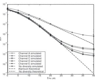
Table 14 summarizes the throughput and C/N thresh-old obtained for each simulated scenario in AWGN chan-nels. It can be seen that the scenario with 16-QAM mod-ulation and LDPC code rate 3/4 has the same throughput of the scenario with 64-QAM and code rate 1/2, but it has lowerC/Nthreshold and, thus, better performance.

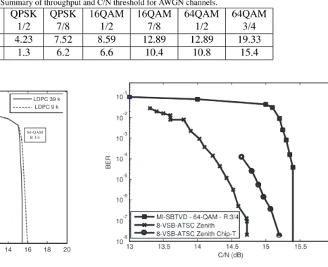
In order to investigate the influence of the LDPC block length codes, Figure 19 compares the performance of the system considering 64-QAM, 16-QAM and QPSK mod-ulations and LDPC with lengths equal to 9k and 39k with rates equal to12and

3

4. It can be seen that the performance

is only 0.2 dB better if a 39k LDPC code is used, instead of the 9k LDPC code specified for the MI-SBTVD sys-tem.

Figure 20 compares the performance of the proposed system with the results presented in [23] for the ATSC standard. It can be observed that both systems have sim-ilar performances. However, it is important to notice that our results have been obtained by simulation and that the results presented in [23] have been obtained from mea-surements. Thus, we can expect that the performance of the ATSC would be better than the performance of our system in AWGN channel. Actually, the ATSC has the best performance in this kind of channel.

(16)

Table 14. Summary of throughput and C/N threshold for AWGN channels.

QPSK QPSK 16QAM 16QAM 64QAM 64QAM

1/2 7/8 1/2 7/8 1/2 3/4

Throughput [Mbps] 4.23 7.52 8.59 12.89 12.89 19.33

C/NNthreshold[dB] 1.3 6.2 6.6 10.4 10.8 15.4

LDPC 39 k

QPSK R 1/2

16-QAM R 1/2

64-QAM

R 1/2 _64-QAM

R 3/4 LDPC 9 k

0 16 20

BER

2 4 14 18

C/N 100

10-1

10-2

10-3

10-4

10-5

10-6

12 10 8 6

Figure 19. Comparing the influence of the LDPC block lengths.

BRAZIL-ECHANNELS

Since the proposed system uses two transmitting an-tennas by default, it was necessary to choose a phase de-lay profile for the two channels of the Alamouti scheme. The phase delays used to generate the performance curves presented in this section were chosen at random, with no loss of generality, because, in all cases studied, a differ-ence of only about 0.6 dB was observed between the best and the worst performances.

Figure 21 shows the performance of the system for ex-ternal line-of-sight reception, corresponding to Brazil-A channel. TheC/N threshold observed ranges from 15.75 dB, for 64-QAM modulation with code rate 3/4, down to 6.9 dB, with QAM with code rate 1/2. We note that 16-QAM with code rate 7/8 has worse performance, in terms ofC/Nthreshold for the same throughput, than 64-QAM with code rate 1/2, indicating that it is not very useful as a transmission mode. The performance of the transmission system was also studied for channels B through E using the configurations above. Figure 22 shows the results for 64-QAM modulation with code rate 3/4. It can be seen that the system can work with throughput greater than 19 Mbps andC/Nlower than or equal to 18 dB in all chan-nels.

Figures 23, 24, 25 and 26 compare the performance between MI-SBTVD, ISDB-T and DVB-T standards for channels Brazil-A, Brazil-B, Brazil-C and Brazil-E. All

13 13.5 14 14.5 15 15.5 16

10-8 10-7 10-6 10-5 10-4 10-3 10-2 10-1

C/N (dB)

BER

MI-SBTVD - 64-QAM - R:3/4 8-VSB-ATSC Zenith 8-VSB-ATSC Zenith Chip-T

Figure 20. Comparing the performance between MI-SBTVD and ATSC in AWGN channel.

comparisons consider 64-QAM modulation and LDPC code rate 3/4 for the MI-SBTVD system. One can see that the proposed system performs better than ISDB-T and DVB-T standards. The difference in the performances varies from 6 dB to 19 dB. Again, it is important to notice that the performance of the proposed system has been ob-tained by simulation and the results presented in [23] for ISDB-T and DVB-T have been obtained from measure-ments.

5.3. PERFORMANCE ON CHANNELS WITH IMPUL

-SIVENOISE

The basic test procedure for channels with impulsive noise was to find, for each value of carrier-to-interference ratio (C/I), the minimumC/Nratio that results in a BER of at most 3 ×10−6

(17)

4 6 8 10 12 14 16 10-6

10-5 10-4 10-3 10-2 10-1 100

C/N (dB)

BER

16QAM - R:1/2 16QAM - R:7/8 64-QAM - R:1/2 64-QAM - R:3/4

Figure 21. System Performance for Brazil-A Channel.

greater than or equal to 26.5 dB, approximately.

Figure 28 shows the performance of MI-SBTVD un-der the presence of impulsive noise consiun-dering the chan-nel IMPUL-O, for 64-QAM modulation and LDPC code with rate 3/4, which presents throughput greater than 19 Mbps. It can be seen that the proposed system is able to operate with BER smaller than TOV for C/I ratios greater than or equal to 33.5 dB, approximately.

5.4. INFLUENCE OF THE ALAMOUTI’SSCHEME IN

THESYSTEMPERFORMANCE

To evaluate the efficiency of the Alamouti space-time coding scheme, the 2x1 mode was compared to the 1x1 mode using 64-QAM with rate 3/4 for Brazil-A through Brazil-E channels. An example of the obtained results is presented in Figure 29 for the Brazil-A channel. The performance improvement obtained with the use of two antennas was substantial, with gains ranging from 1.9 dB, for Brazil-C channel, up to 4 dB for Brazil-B channel.

5.5. MOBILERECEPTIONPERFORMANCE

The channel model that represents mobile reception is typical urban GSM. Two mobility scenarios have been considered: one with low speed (around 25 kilometers per hour for the UHF channel 14) and another one with high speed (around 130 kilometers per hour for the UHF chan-nel 14). In all figures presented in this sub-section,the value of theC/N threshold is the last point on the curve. The vertical line down from that point indicates that it was

12 13 14 15 16 17 18 19

10-7 10-6 10-5 10-4 10-3 10-2 10-1 100

C/N (dB)

BER

Canal A Canal B Canal C Canal D Canal E

Figure 22. System Performance for Brazil-A through Brazil-E channels using 64-QAM and LDPC code rate 3/4.

13 14 15 16 17 18 19 20 21 22

10-8 10-7 10-6 10-5 10-4 10-3 10-2 10-1 100

C/N(dB)

BER

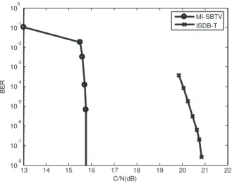
MI-SBTV ISDB-T

Figure 23. Comparing the performance between MI-SBTVD and ISDB-T for Brazil-A Channel.

(18)

14 16 18 20 22 24 26 10-7

10-6 10-5 10-4 10-3 10-2 10-1 100

C/N(dB)

BER

MI-SBTV ISDB-T

Figure 24. Comparing the performance between MI-SBTVD and ISDB-T for Brazil-B Channel.

14 16 18 20 22 24 26

10-8 10-7 10-6 10-5 10-4 10-3 10-2 10-1 100

C/N(dB)

BER

MI-SBTV ISDB-T

Figure 25. Comparing the performance between MI-SBTVD and ISDB-T for Brazil-C Channel.

presented here, it can be concluded that the system is able to operate with high efficiency for mobile reception using more robust modulation schemes, such as QPSK and 16-QAM. Figure 34 compares the performance of the system with two transmitting antennas when one of the antennas is turned off (without any change at the receiver). The configuration with QPSK modulation, code rate 1/2 and Doppler deviation of 60 Hz was used. Similar results to the ones shown in Figure 34 were obtained for 16-QAM modulation, code rate equal to 1/2, and Doppler deviation 12 Hz. From these results, it is possible to observe a drop of 5-9 dB on the system performance when one of the transmitting antennas is turned off.

15 20 25 30 35

10-8 10-7 10-6 10-5 10-4 10-3 10-2 10-1 100

C/N(dB)

BER

MI-SBTV DVB-T

Figure 26. Comparing the performance between MI-SBTVD and DVB-T for Brazil-E Channel.

26 28 30 32 34 36 38

10 11 12 13 14 15 16

C/I (dB)

C/N (dB)

Figure 27. Performance with impulsive noise and internal reception.

6. I

MPLEMENTATION

A

SPECTS

This section introduces some implementation tech-niques which were chosen to exemplify what kind of algo-rithms engineers have to deal with when designing a phys-ical layer system for ASIC or FPGA, particularly when the target application is digital television. Although the algorithms are presented here using a systemic approach, they can also encompass behavioral abstractions, includ-ing loop controls and processes. The behavioral approach is typically used for synchronous operations such as fil-tering or any other digital signal processing algorithm.

(19)

ca-32 34 36 38 40 42 44 15

16 17 18 19 20 21 22

C/I [dB]

C/N [dB]

Figure 28. Performance with impulsive noise and external reception.

13 14 15 16 17 18 19 20

10-6 10-5 10-4 10-3 10-2 10-1

C/N (dB)

BER

Alamouti 1x1 Alamouti 2x1

Figure 29. Comparing the performance between Alamouti 1 x 1 and 2 x 1 over Brazil-A channel.

pacity. Perhaps the greatest challenge in the design of new algorithms for an FPGA is the trade-off between high speed processing and silicon area occupation.

For example, when a Cordic division algorithm, which is very expensive in logical resources (silicon area), needs to performN divisions in a given time slot, it may not have enough hardware resources to implement all theN

operations in parallel. In this case, some operations have to be serialized, increasing the clock, to implement the di-vision algorithm in a semi-sequential or totally sequential mode.

Another example is the implementation of an LDPC decoder using an eIRA code for rate 3/4 and codeword

0 5 10 15 20 25

10-6 10-5 10-4 10-3 10-2 10-1 100

C/N [dB]

BER

Correlation = 0 Correlation = 0.2 Correlation = 0.6

Figure 30. Mobile reception with 16QAM, R = 1/2 and Doppler deviation equal to 12 Hz.

2 4 6 8 10 12 14

10-7 10-6 10-5 10-4 10-3 10-2 10-1

C/N (dB)

BER

correlation = 0 correlation = 0.2 correlation = 0.6

Figure 31. Mobile reception with 16QAM, R = 1/2 and Doppler deviation equal to 60 Hz.

length of 9792 bits [26]. The implementation of such a decoding algorithm in an FPGA Xilinx Virtex 4 SX35 is not feasible with a full parallel architecture. For this rea-son, a semi-sequential approach, in the form of a trellis structure, had to be used with a parallelization degree of 51, a number just sufficient to fit the algorithm in the de-vice.

(20)

2 4 6 8 10 12 14 16 10-6

10-5 10-4 10-3 10-2 10-1

C/N (dB)

BER

correlation = 0 correlation = 0.2 correlation = 0.6

Figure 32. Mobile reception with QPSK, R = 1/2 and Doppler deviation equal to 12 Hz.

2 4 6 8 10 12 14

10-7 10-6 10-5 10-4 10-3 10-2 10-1

C/N (dB)

BER

correlação = 0 correlação = 0.2 correlação = 0.6

Figure 33. Mobile reception with QPSK, R = 1/2 and Doppler deviation equal to 60 Hz.

is responsible for integrating the video generation, the channel encoding and the modulation sub-systems in the transmitter prototype.

6.1. DIGITALDOWN-CONVERTER

The receiver design was based on a software defined radio (SDR) architecture and consists basically of a super-heterodyne receiver, with the IF stage implemented dig-itally in software, as shown in Figure 35. In a super-heterodyne scheme, the receiver front-end is typically split into an RF and an IF stage, as shown in Figure 36.The RF stage is sensitive to a wide frequency range, in

2 4 6 8 10 12 14 16 18 20

10-7 10-6 10-5 10-4 10-3 10-2 10-1

C/N (dB)

BER

Alamouti 2x1 - correlation = 0 Alamouti 2x1 - correlation = 0.6 Alamouti 1x1

Figure 34. Mobile reception with QPSK, R = 1/2 , Doppler deviation equal to 60 Hz and Alamouti 1x1 and 2x1.

our case 30 MHz, and may have one or two tuned stages which are necessary to allow television viewers to select the desired channel. After a channel is selected by ad-justing the local oscillator frequency, the incoming signal is multiplied by the oscillator signal in a mixer, which results in down-converting this incoming signal to an in-termediate frequency (IF). In the IF stage, the signal is filtered to extract the desired channel, allowing the rest of the circuitry to be sensitive to a shorter frequency range, in our case 6 MHz. Finally, the resulting signal is down-converted to baseband and can be demodulated by soft-ware.

There are many advantages in the use of a SDR re-ceiver compared to a traditional super-heterodyne archi-tecture, such as:

• The digital down-converter eliminates the draw-backs of phase and gain mismatch associated with its analog version. The local oscillator, used in the ana-log down-conversion, is replaced by a simple look-up table containing samples of a sinusoidal wave, as shown in Figure 37. All operations are digitally im-plemented, which avoid unbalancing the in-phase (I) and quadrature-phase (Q) baseband signals.

• Channelization can be implemented in software by digital low-pass filtering. The analog version of this process demands for analog filters with very strin-gent requirements, which are much more difficult to implement compared to their digital versions.

(21)

LNA Filter

LO

AGC + amplifier Filter

ADC

Digital Baseband Processing Digital

Down-Converter

RF IF BB

Figure 35. Software-defined radio architecture.

LNA Filter

LO

AGC + amplifier Filter

90º Filter

Filter VCO

ADC

ADC DAC

Digital Baseband Processing

RF IF BB

in-phase signal

quadrature signal

Figure 36. Traditional super-heterodyne receiver.

prototype of the MI-SBTVD system was chosen to oper-ate with an IF of 8.1270 MHz, which corresponds exactly to the same sample frequencyfsused for I and Q base-band signals. The reason for that choice is that, when the analog signal is sampled with 4fs, the digital mixing has a very simple structure, as shown in Figure 38, which re-places the look-up tables and the two multiplications by a simple switch and a “negate" operation (times -1). If the intermediate frequency isfs, then it is necessary to mix the sampled IF signal with two quadrature sinusoidal waves of frequencyfs, in order to recover the baseband signals. These sinusoidal waves need to be sampled at the same rate 4fs as the input signal, which results in two periodic sequences: 1, 0, -1, 0 for the cosine wave and 0, 1, 0, -1 for the sine wave. The mixing operation is performed by multiplying the IF signal with these two periodic sequences, 1, 0, -1, 0 and 0, 1, 0, -1, in the I and Q branches, respectively. To save computational ef-fort, a switch is used in each branch, splitting the samples multiplied by 1 and -1 and the samples multiplied by 0. Subsequently, a low pass filter with a polyphase structure is used to decimate the mixed signal, resulting in the I and Q signals at baseband sampling ratefs. The advantage of

using polyphase decimators is that the filtering operation is performed on the lower baseband frequencyfs, which also saves computational effort [24] [25].

Counter 0,1,.., N-1

Input

N-samples Look-up table

(cos)

N-samples Look-up table

(sin)

LPF

I

Q addr

addr

cos(2 n/N)

sin(2 pin/N) pi

Figure 37. A digital down-converter implementation using look-up tables.

(22)

Counter 0,1, 2, 3

Input

LPF I

Q sel

LPF sel

cos(2 n/4) = [1 0 -1 0]

sin(2 n/4) = [0 1 0 -1]

-1

0

0 switch

switch pi

pi

Figure 38. A low-complexity implementation of a digital down-converter scheme.

SYSTEM

The main idea for rate control is to transmit null data packets, that is, packets which do not have useful infor-mation, always when new data is required by advanced stages and that required data is still not available to be processed. This occurs, for example, when the video data rate to be transmitted is below the system throughput, which forces the system to fulfill the difference with some dummy information, in this case the null packets, which can be identified and later removed at the receiver. We, therefore, have two types of packets which can be trans-mitted. Besides, once the transmission of one packet type has started, it is necessary to complete that transmission before switching to another packet type. Although this rule might sound obvious, it is very important not to mix the two packet types together, otherwise the null ones will not be recognized by the receiver and consequently they cannot be removed. Obviously, this will corrupt the video data, since the receiver will not be able to restore the orig-inal video stream.

In this way, two states can be defined for the rate con-trol algorithm: “read data packet" and “read null packet". These states are imbedded in the register “Reading State", which stays in the same state at least during 204 valid con-secutive bytes, which is the packet size for both packet types. The purpose of this register is to inform if there is an entire data packet available for reading, and its content is always updated whenever the last byte of one packet is read by the system. Therefore, whenever a new packet is about to be read, that is, when the “frame index" reaches the value 203, the control signal “Data Packet Available" is inspected and saved in the register “Reading State".

With these concepts in mind, it is easier to understand the control signals of the algorithm, as shown in Figure 39. The “Reading State" controls the selectors “Data

Selector" and “Valid Selector", which drive the outputs “Byte Output" and “Valid Output", respectively. When the state is “0", that is, when there is no data available for reading, then a null packet is read through a ROM memory. The reading address is provided by the counter “frame index" and the signal “Valid" is a delayed version for the reading request coming from the LDPC encoder.

On the other hand, when the “Reading State" is “1", it means that there is at least one data packet available for reading, and then the signal “Reading Request", coming from the LDPC encoder, is passed as a read enable control to the input FIFO (First In First Out) which records the data packets. This FIFO is not shown in Figure 39, but in Figure 40. As a result, the bytes read from this FIFO are made available on the input ports “Input Byte" and “Input Valid". The latter signal “Input Valid" is redundant here because it is always “1" when the “Reading Request" is “1", and “0" otherwise.

3 Request data to input FIFO

2 Valid Output

1 Byte Output

sel

d0

d1

Valid Selector d

en q

z-1

Reading State

addr z-1

Null Packet ROM

and

z-0

en out

Frame Index : count from 0 to 203 bytes

sel

d0

d1

Data Selector 203

a

b

a=b

z-0

Compare

dz-1q

Alignment2

d z-1 q

Alignment 4

Reading request from LDPC

encoder 3 Data packet

is available

2 Valid from

FIFO 1 Data from

FIFO

Figure 39. Block diagram showing the implementation of the rate control system. This block diagram is implemented using Xilinx

System Generator for Matlab/Simulink.

Now, we present how the rate control is used to pro-vide a continuous data flow at the output of the trans-mission system. The transtrans-mission system, as shown in Figure 40, is a particular implementation of the proposed MI-SBTVD system, and has been successfully tested in an FPGA Xilinx Virtex 4 SX35. The simplification has been made in order to present an instructive approach without loss of generality. Besides, this version also does not include RS coding and interleaver and operates under only one transmission mode (64 QAM, guard interval of 1/16, LDPC 3/4, 2048 carriers), providing a throughput of 19.33 Mbps.