J. Braz. Soc. Mech. Sci. & Eng. vol.27 número4

(1)

R. G. R. Camacho

and J. R. Barbosa

Instituto Tecnológico de Aeronáutica 12228-900 São José dos Campos, SP. Brazil ramirez@ita.br rgramirez65@hotmail.com barbosa@ita.br

The Boundary Element Method

Applied to Incompressible Viscous

Fluid Flow

An Integral equation formulation for steady flow of a viscous fluid is presented based on the boundary element method. The continuity, Navier-Stokes and energy equations are used for calculation of the flow field. The governing differential equations, in terms of primitive variables, are derived using velocity-pressure-temperature. The calculation of fundamental solutions and solutions tensor is showed. Applications to simple flow cases, such as the driven cavity, step, deep cavity and channel of multiple obstacles are presented. Convergence difficulties are indicated, which have limited the applications to flows of low Reynolds numbers.

Keywords: Boundary elements, fundamental solution, integral equations

Introduction

The need of solution of the system of partial differential equations which model the flow of a fluid in channels such as pipes, blade passages, nozzles and others appeared the very first day the fluid flow was modeled. The difficulties involved in obtaining closed solutions, even for very simple flows, required the development of clever techniques, but only with the application of numerical solutions to that system of equations, some flows of practical interest were calculated.

Several computational techniques have been used: finite difference, finite element, finite volume and boundary element to name the most known. As new algorithms were discovered and faster computers were produced, each of those methods evolved in all areas in the past years. Finite difference methods have been, implemented to solve flow problems. Finite elements gained attention in the past decades; in the seventies it was still crawling. Both are bases for commercial codes for the solution of flows of almost every kind. Computer effort has been limiting the application of the numerical methods in the sense that every new discovered method of solution claims reduction in CPU time and storage requirements. 1

The boundary element method, nevertheless, has progressed differently depending on the areas where it has been applied. It has been developed fastest in areas related to solid mechanics and acoustics problems, (Brebbia and Walker 1980; Brebbia, Telles and Wrobel 1984; Banerjee and Butterfield 1981) and slowest in the fluid mechanics.

A didactical approach is used in this work. The method of the boundary elements is applied to fluid problems, aiming also at introducing the methodology to new users. The computational implementation is based on the Kakuda and Tosaka (1988) reports. There, the boundary element method uses a reformulation of the unsteady Navier Stokes equations in terms of velocity components only, by making use of the penalty function method, an approach successfully applied to flow analysis with finite element. The effectiveness of this method was illustrated by several numerical examples. Tosaka and Onishi (1985, 1986) proposed new integral representations for the Navier Stokes equations for both steady and unsteady flow problems. The workability and validity of the methodology developed therein were shown with several numerical results for steady problems (Tosaka, Kakuda and Onishi (1985); Tosaka and Kakuda (1986); Tosaka (1986)).

Paper accepted July, 2005. Technical Editor: Aristeu da Silveira Neto.

Although integral methods were available many decades ago for the application to flow problems of practical interest, a comprehensive study of the formulation and application to flow problems are still being considered more recently, as they are expected to alleviate sensibly the storage and hopefully CPU time, Despite this apparent advantage, requiring less computational effort when volume integrals are transformed into surface integrals, some disadvantages arise, such as higher mathematical complexity in order to get an usable computational formulation; the need for the calculation of singular integrals; dense matrices whose inversion is more time consuming when comparable with the banded matrices in the finite difference and finite element schemes.

In the section Application below the application of the boundary element method to the following fluid problems are shown: a) stepped channel, b) box with moving lid, c) channel flow with multiple obstacles, d) deep cavity flow e) channel flow with heat transfer.

Nomenclature

ρ = density

µ = dynamic viscosity P = pressure

T = temperature ν= absolute viscosity

k= thermal conductivity

v

c = specific heat at constant volume

p

c = specific heat at constant pressure

Statement of the Problem

Let Ω be a domain in 2

R and Γ its closed boundary; ni be the

outer normal vector to the boundary; the fluid be a perfect gas,

incompressible and viscous; (x,y) be a point of Ω in R . The steady 2 state conservation equations in cartesian co-ordinates can be written as:

Conservation of Mass:

0

= ∂ ∂ + ∂ ∂

y v

x u

(2)

Copyright  2005 by ABCM Conservation of Momentum:

x - direction

      ∂ ∂ + ∂ ∂ ρ = ∂ ∂ −               ∂ ∂ + ∂ ∂ ∂ ∂ + ∇ µ y u v x u u x P y v x u x u 2 (2a) y-direction       ∂ ∂ + ∂ ∂ ρ = ∂ ∂ −               ∂ ∂ + ∂ ∂ ∂ ∂ + ∇ µ y v v x v u y P y v x u y v 2 (2b)

Conservation of Energy:

      ∂ ∂ ∂ ∂ ρ ∇ y T v + x T u v c = T 2 k (3)

Let the following change of variables take effect in the conservation equations:

L tV t*= ∞

2 * ∞ ∞ ρ − = V P P P ∞ ρ ρ = ρ* L y y*=

∞ = V u u* ∞ = V v

v* V_∞ = u_∞2 +v_∞2

∞ µ µ = µ* ∞ ν ν = ν*

where ∞ refers to the far stream condition; and Re and Pr are the Reynolds and Prandtl numbers, respectively.

Then, the conservation equations become:

Conservation of Mass

0 * * = ∂ ∂ + ∂ ∂ y v x u (4)

Conservation of Momentum

x-direction         ∂ ∂ + ∂ ∂ = ∂ ∂ −         ∂ ∂ + ∂ ∂ ∂ ∂ + ∇ * _** * * * * * * * * * * * 2 Re Re y u v x u u x P y v x u x

u (5a)

y-direction         ∂ ∂ + ∂ ∂ = ∂ ∂ −         ∂ ∂ + ∂ ∂ ∂ ∂ + ∇ * _** * * * * * * * * * * * 2 Re Re y v v x v u y P y v x u y

v (5b)

Conservation of Energy

        ∂ ∂ + ∂ ∂ = ∇ − * _* * * * * 2 Pr Re 1 y T v x T u T (6)

For the sake of simplicity, the asterisk will be dropped in what follows.

The independent variables of the problem are u, v, T and P. It is possible to rewrite the conservation equations in matrix form as

[L] {U} ={B} (7)

where [L] is a linear partial differential operator, {U}=

{

}

T

P T v

u is the vector of the unknowns and {B} the vector of nonlinear convected terms. Depending on the assumptions made, [L] and {B} can take different forms. For instance, vector {B} can be linearised and the linear terms included in [L].

Let, for the moment, all non-linear terms are included into {B}. Then                   ∇ − + ∇ − + ∇ = 0 0 0 Re 1 0 0 Re 0 Re 0 2 1 2 2 2 2 2 1 2 1 2 1 1 1 2 IJ D D D D D D D D D D D D L ;               = P T v u

U_J ;

                              ∂ ∂ + ∂ ∂       ∂ ∂ + ∂ ∂       ∂ ∂ + ∂ ∂ 0 Pr Re Re = I y T v x T u y v v x v u y u v x u u

B . (8)

(I, J=1, 2, 3, 4)

Where: x D ∂ ∂ = 1 ; y D ∂ ∂ =

2 ; 2 2 2 2 2 y x ∂ ∂ + ∂ ∂ = ∇ (9) The Method

Equation (7) has no known solution. Let U~_J be an approximate

solution in the sense ofLIJU~J −BI =R≅0, that is, UJ ~

differs

from U_J very little but it is not equal to U_J.

In order to derive the integral equation for steady-state problem, the method of weighted residual is applied. The weighted residual statement for Eq. (7) can be expressed as

(

)

∫

Ω

= Ω

−B W d 0

U

LIJ J I IK (10)

A possible solution can be obtained provided theW_IKas an appropriate weight function. It will be shown later that W_IKis

chosen as the fundamental solution tensor for the adjoint ofLIJ. Hörmander´s (1965) (Banerjee, 1994) method is used for the calculation of the weight functionW_IKtensor and fundamental

solution. Although it does not provide WIK directly, it allows, as a first step, the combination of several partial differential operators

IJ

L into a single differential operator, from which the tensor W_IK

is calculated. The weight tensor W_IKor the fundamental solution may be determined as a solution of steady Stokes problem with heat transfer: 0 ) ( − = δ δ

+ x y

W

(3)

whereδ(x−y) is the Dirac delta function and L_IJ is the adjoint operator of L_IJ.

Hörmander’s method is simultaneously applied to the continuity, Navier Stokes and energy equations for steady, incompressible flow: ) ( ] [ ] ][

[L W =− I δx−y (12)

Multiplication of equation (12), to the left, by [L]−1 results: ) ( ] [ ) ( ] [ ]

[W =− L −1δx−y =− I δ x−y (13)

where, [L]−1=Adj[L]/Det[L] and Adj[L]=CofT

[ ]

L

                  ∇ ∇ ∇ ∇ ∇ ∇ ∇ ∇ ∇ ∇ ∇ − ∇ ∇ − ∇ ∇ − ∇ − ∇ = 2 2 2 2 2 2 2 2 1 2 2 2 2 2 2 2 1 2 2 1 2 2 1 2 1 2 2 2 2 T Re 2 0 Re 1 Re 1 0 Re 0 0 0 0 ] [ Cof D D D D D D D D D D

L (14)

whose terms are xij=(−1)(i+j)mij;mijare the minors of [L], and

[ ]

2

(

2

( )

2

)

detL =∇ ∇ ∇ (15)

Thus,

[ ]

(det ) [ ] ( ) Cof ) ( ] [ ]

[W = L −1δx−y = T L L −1 I δx−y (16)

Let ) ( ]) [ det ( 1 * y x

L δ −

=

φ − (17)

then

) ( ] [

det L φ*=δx−y (18)

whose solution φ* is:

r r y x ln 128 1 ) , ( 4 * π = φ (19)

where r= x−y denotes the distance between x and y (Tosaka,

1989).

Therefore, the fundamental solution tensor W_JKcan be determined explicitly from equations (16) and (18) in conjunction with (19) as follows:

        ₋ + + π

= ₂ 2

11 ) ( 1 ) ln( 4 1 r y y r

W i 

     − π − = ₂ 42 ) ( 2 1 r y y W i       − − π − = 2 21 ) ( ) ( 4 1 r y y x x

W i i W13=W23=W43

0 31=

W (3 2ln )

4 Re 33 r W + π =       − π = ₂ 41 ) ( 2 1 r x x

W i 

     − π = ₂ 14 ) ( Re 2 1 r x x W i 21 12 W

W = _

     − π = ₂ 24 ) ( Re 2 1 r y y W i         ₋ + + π

= ₂ 2

22 ) ( 1 ) ln( 4 1 r x x r

W i W₃₄ =W₄₄

0

32=

W (20)

Important to notice that, the tensor WJKcalculation is only determined analytically, this way, it is important to be careful in the obtaining of these equations.

Discretization

Let the Green-Gauss theorem be applied to equation (10) so that the domain integral is transformed into an integral over the contourΓ, divided into ne boundary elements. Then,

(

)

∫

Ω

= Ω

−B W d 0

U

L_IJ _J _I _IK (I, J, K=1, 2, 3, 4) (21)

which tells that the system of differential equations has been transformed into a system of algebraic equations (21) that involves the values of the variables at each boundary element. If one finds the values of the variables at the elements in the boundary, the solution in the boundary is then obtained.

After the application of the Green-Gauss theorem and integrating by parts over Ω, one arrives at the following equation that holds for every boundary element as well:

{

}

∫

Ω Γ Γ Ω + Γ       − ∂ ∂ + + Γ τ − Σ = ) ( ) , ( ) ( ) ( ) , ( ) ( ) , ( ) ( ) ( Re 1 ) ( ) , ( ) , ( ) ( ) ( ) ( 3 3 x d y x W x B x d y x W x q y x x n W x T x d W y x y x x u y U y C IK I K K IK i IK i I KI (22)

where summation is implied by repeating indices.

It is work mentioning that right hand side of equation (22) comprises integrals over the boundary and over the domain, these due to the non-linear convective terms,BI.

In equation (22),C_IKis the tensor coefficient dependent on the geometry of the boundary. Its value is ½, 1 or 0, provided the point

y lies over a locally regular boundary, within the domain or outside the boundary, respectively. If y lies at a corner of Γits value is

π

α 2 , where α is the angle formed by the left and right tangents to Γ. Also,

n x T x q ∂ ∂ = ( ) ) ( (23) j i jK j iK ij K

iK(x,y)=(−W4 δ +W , +W ,)n

Σ (24) j i j j i ij

i(x)=(−Repδ +u, +u , )n

(4)

Copyright  2005 by ABCM where coma (,) stands for derivative with respect to the following

index and summation is implied by repeating indices. From equation (24) the values of ∑_IK are calculated:

(

14 2( )( )

Re 1 n r y y x x n r y y r x

x _i _i _i _i

(26)

For constant boundary element, one has

( )

       = Γ = Γ τ = Γ τ = Γ e e e e i e i i e i q q T T u u e e (27)

Substituting the indicated expressions into equation (22):

( ) ( )

{

( )

}

( )

_{( )}

( ) ( ) ( )

∫

∑ ∫

Ω = Γ = Γ Ω + + Γ       − ∂ ∂ + + Γ τ − Σ = x d y x W x B d q y x W T n y x W x d x y x W x u y x y U y C Ik I n e e e K e K n e e i iK i iK I KI e , , , Re 1 ) ( ) ( , ) ( , 2 2 1 3 3 1 (28)

Equation (28) can be rewritten after substitution for the constant terms listed in equation (27), from what results a system of algebraic equations.

Numeric Implementation

Boundary: Let Γ be the boundary, divided into m constant elements, with the collocation points (nodes) located at mid position of each element. Application of equation (28) to m nodes gives a set of 4m equations with 4m unknowns. For the solution of this system of equations two auxiliary matrices are assembled, for each element:

( )

x y

n W y x Y X

G iK K ,

Re 1 , ) ( 3 ∂ ∂ − Σ = − βα (29)

(

X Y

)

W

( )

x y W

( )

xy

H iK K ,

Re 1 , − 3 = − βα (30) from which

(

)

∫

Γ βα Γ − = αβ e e e _Y _G _X _Y _d

g ( ) (31)

(

)

∫

Γ βα Γ − = αβ e e e _Y _H _X _Y _d

h ( ) (32)

Integrals (31) and (32) are carried out numerically, using one-dimensional Gaussian quadrature, if X≠Y. When X=Y, the integrands of (31) and (32) become singular, requiring the calculation in the sense of Cauchy principal value. Among several techniques available to perform these calculations, in this work the method of Telles (1987) was chosen.

Domain: To calculate the integrals over Ω, the domain is subdivided into M elements by an appropriate net. Triangular cells will be used in this work. Let ωj be the Gauss weight function at

point j, SΩe the area of element e, and J the number of Gauss integration points. Then

( ) ( ) ( )

xW x yd x

(

BW

( )

x y

)

S _e B M e J j j IK I j Ik I Ω = = Ω

∑ ∑

∫

_       ω = Ω 1 1 , , (33)

Gauss quadrature with seven integration points in each triangular cell of the sub domain, and the Hammer technique, as described by Partridge et al (1992), are used to determine the domain integral.

In equation (28) the values ui and T are known;

τ

i and qi are unknown gradients of velocity and temperature.

Defining

[

]

T

1 1

1v T um vmTm u

=

δ (34)

τ=

[

τ₁₁τ₂₁q₁ τ₁_mτ₂_mq_m

]

T (35)

equation (29) can be rewritten as

} { } { ] [ } { ] [ } { ]

[C δ + H δ = G τ + D (36)

Defining ] [ ] [ ]

[H = C − H

one arrives at

} { } { ] [ } { ]

[H δ = G τ + D (37)

Boundary conditions: For the application of the boundary conditions to equation (37), it is worth noting that elements of δ and of τ have some prescribed values. It is therefore convenient to rearrange δ and τ in such a way that the unknowns come first and then the prescribed values, that is,

[

]

T

p u δ δ = δ

τ=

[

τ_u τ_p

]

T (38)

Rearrangement of matrices[H], [G] and {D} accordingly, results in

(5)

Rearrangement of equation (39) such that only the unknowns are in the left hand side of the equation, gives

} { } { ] [ } ]{

[A X = B P + D (40)

Matrix [A] is dense so that inversion is time consuming. The inversion is carried out using the Gauss elimination algorithm. Solution of equation (40) gives the values of the unknowns at the boundary.

Computer Program: A modular computer program has been developed that is able to handle geometries composed of rectangles, written in FORTRAN and run in a 2.0 GHz personal computer.

The computer program implementation was carried out with the following steps:

- Definition of the geometry by a combination of rectangles. - Boundary discretization using elements of same size. - Domain grid generation using triangular elements. - Numbering elements counterclockwise.

- Imposition of the boundary conditions and initialization of domain variables (velocity, temperature and pressure) using reasonable guesses according to the problem being solved. - Assembly of matrices ge_αβ and he_αβ for each element e. - Assembly of matrices [G] and [H] for all elements on the

boundary.

- Numeric evaluation of domain integrals (equation (33)). - Solution of equation (40) for the determination of the

variables at the boundary.

- Solution of equation (22) at internal nodes, with CKI=1. More details about computational implementation can be found in the Santos (1998) and Ramirez et al (2004)

Application

For the demonstration of applicability of the method, five problems were chosen:

a) the recirculating flow in a square cavity driven by a lid sliding at uniform velocity;

b) the flow facing a forward step; c) the flow over a deep cavity and

d) the flow over a deep cavity with the upper surface at a higher temperature;

e) the flow in a channel with multiple obstacles.

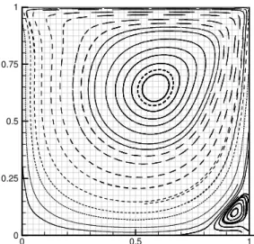
Driven cavity flow: The flow in the box is depicted using streamlines, as shown in Fig. 1. The boundary conditions are the no-slip in the box boundaries, that is, zero at the non moving surfaces and the velocity of the moving slid at the upper surface. Constant temperature was set on the boundary. Grid for Fig. 1a is 40x40 and for Fig. 1b is 30x30. Criteria of convergence were based on the difference ε of the previous and the actual calculated values for velocities, pressure and temperature. Convergence was achieved up to Reynolds number of 400. Recirculation is detected at the bottom-right of the cavity.

Flow in a stepped channel: Streamlines of the flow in a forward facing step is shown in Fig. 2a. Boundary conditions are: parabolic distribution of velocities at inlet, no-slip condition on the walls and constant wall temperature. The results shown are for a grid of 26×30. The predicted reattachment point is in agreement with other predicted numeric methods such as the finite volume methods (Fig 2.b), (Rocamora F, 2002)

0 0.5 1

0 0.25 0.5 0.75 1

Figure 1a. Streamlines in the driven cavity flow Re = 300, grid 40××××40,

εεεε=0.0001.

0 0.5 1

0 0.25 0.5 0.75 1

Figure 1b. Streamlines in the driven cavity flow Re = 400, grid 30××××30,

εεεε=0.001.

. 00 1 2 3 4 5 6

0.5 1 1.5 2

Figure 2a. BEM. Streamlines in the channel flow Re = 30, grid 26××××30,

∈ ∈ ∈ ∈=0.0001.

0 1 2 3 4 5 6

0 0.5 1 1.5 2

(6)

Deep cavity flow: The streamlines for Re=10, grid 40×40 and

ε=0.0001, are shown in Fig. 3a, which is a good result. In Fig. 3b one can also see satisfactory results with a moderately refined mesh with a grid of 20×20 and ε=0.00001, so that it is possible to obtain good results in shorter processing time. For methodology validation, the finite volume method was used 40×40 elements with refined grid in the corner regions (Figure 3c). The CPU time for the method of boundary elements is smaller for the boundary element method. In Fig. 4 are shown the velocities at the middle of the cavity, obtained from BEM and FVM. It is important to notice that the Boundary Element Method with a grid of 20×20 gives good result when compared to the Method of Finite Volumes. Since convergence is achieved only for low Reynolds number, this formulation is not appropriate for the study of flow in turbomachines, one of our goals. Therefore, research is being carried out order to linearize {B} (Eq.10) and to incorporate those non-linear terms to the linear operator [L]. This method may become very attractive since it is expected to sensible reduce computational cost.

0 1 2 3 4

0 0.5 1 1.5 2 2.5 3 3.5 4

Figure 3a. Streamlines in the deep cavity flow Re = 10, grid 40x40,

εεεε=0.0001.

. 0.0 1.0 2.0 3.0 4.0

0.0 0.5 1.0 1.5 2.0 2.5 3.0 3.5 4.0

Figure 3b. Streamlines in the deep cavity flow Re = 10, grid 20x20,

εεεε=0.00001.

Figure 3c. MFV Streamline in deep cavity flow.

u

y

-0.2 0.0 0.2 0.4 0.6 0.8 1.0 0.0

1.0 2.0 3.0 4.0

FV 40 X 40, F. Rocamola (2002) BEM, 40 X 40, eps=0.0001 BEM, 20 X 20, eps=0.00001

Figure 4. Velocities distribution u in medium section of deep cavity flow. Re=10, grid 20××××20, εεεε= 0.0001.

0 1 2 3 4

1.1 1.3 1.4 1.5 1.6 1.8 1.9 2.0 2.1 2.3 2.4 2.5 2.6 2.8 2.9

T=3.0

T=1.0

T=1.0 T=1.0

T=1.0

(7)

0.0 2.0 4.0 6.0 8.0 10.0 12.0 0.0

0.5 1.0 1.5 2.0

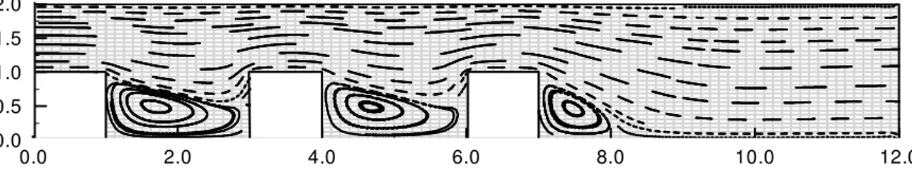
Figure 6. Streamlines in the channel flow with multiple obstacles Re = 20 - grid 26x96, εεεε=0.0001.

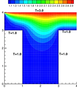
Deep cavity flow (heated upper surface): Although the energy equation had been used in the four previous applications, they were constant temperature applications. In this example, it is shown the variation of fluid temperature in Fig. 5, that shows the temperature contours when the top surface temperature is higher than the temperature of the other surfaces. Again, good results were obtained and no additional CPU time, compared to the previous application, was required.

Channel flow with multiple obstacles: Figures 6 show the streamlines of the flow in a channel with multiple obstacles, for Reynolds numbers 20.

Conclusion

The boundary element method can be applied to the calculation of incompressible viscous flows as demonstrated above. Although coarse grids were used, the results are quite satisfactory, capturing regions of reverse flows. Comparison of CPU times for the BEM and for FVM indicates that the BEM calculations are much faster. It is therefore important to investigate other applications, such as the flow in blade passages, which is the ultimate goal for the research under way. Flow in blade passages require a method that converges for much higher Reynolds number. Such a method is being developed, using linearization of the convective terms to allow the convective information to be incorporated into the fundamental solution and therefore achieve convergence for higher Reynolds numbers.

Acknowledgements

The authors gratefully acknowledge the financial support from FAPESP (Fundação de Amparo à Pesquisa do Estado de São Paulo), El Paso Reference Center for Gas Turbines and ANEEL (Brazilian federal law 9991/2000).

References

Banerjee, P.K., 1994, “The Boundary Element Methods in Engineering”, McGraw-Hill book Company Europe.

Banerjee, P.K., Butterfield, R. 1981 “Boundary Element Methods in Engineering Science”, McGraw-Hill; New York.

Brebbia C. A., Telles T. C. F., Wrobel, L.C., 1984, “Boundary Element Techniques. Berlin. Heidelberg, New York: Springer.

Brebbia, C. A., Walker. S., 1980, Boundary Element Techniques in Engineering. Newnes-Butterworths.

Hörmander, L., 1965, “Linear Partial Differential Operators”, Springer-Verlag, Berlin.

Kakuda, K., Tosaka, N., 1988, “The Generalized Boundary Element Approach For Viscous Fluid Flow Problems”, Boundary Element Methods in Applied Mechanics, Editors: M. Tanaka & T. A. Cruse, Pergamon Press, pp 305-314.

Partridge P.W, Brebbia, C.A., Wrobell L. C., 1992, “The Dual Reciprocity Boundary Element Method”, Computational Mechanics Publications, Southampton.

Ramirez R.G. C., Barbosa J. R., 2004, “The Boundary Elements Method Applied to Incompressible Viscous Fluid Flow Problems”, Anais em CD, III Congresso Nacional de Engenharia Mecânica, Belem – Para.

Rocamora, Jr F. D, De Lemos M J S,. “HeatTransfer Characteristic of Laminar and Turbulent Flows Past a Back Step in a Channel with a Porous Insert”, 9 th Brazilian Congress of Thermal Engineering and Sciences, Caxambu-Minas Gerais, Brasil, 2002.

Santos, Maria de Fatima de Castro Lacaz.,1998, “O Método de Elementos de Contorno Aplicado a Problemas de Escoamento de Fluidos”. Tese Doutorado (Engenharia Aeronáutica e Mecânica) – Instituto Tecnológico da Aeronáutica, (Orientador) J. R. Barbosa.

Telles, J.C.F.A., 1987, “A Self-Adaptive Co-Ordinate Trans-formation for Efficient Numerical Evaluation of General Boundary Element Integrals, Int. J. Numeric Methods in Engineering, 24:pp 956-973.

Tosaka, N. Kakuda, K. & Onishi, K., 1985, “Boundary Element Analysis of Steady Viscous Flows Based On P-V-U Formulation”, Proc. 7nth Conference of BEM in Engineering, Lake Como, 71-80(9), Italy.

Tosaka, N., 1986, “Numerical Methods for Viscous Flow Problems Using an Integral Equation . In: Wang, S.Y., Shen, H.W., Ding, L. Z. (eds): River sedimentation, pp. 1514-1525: The University of Mississippi.

Tosaka, N., Kakuda, K. 1986, “Numerical Solution of Steady incompressible Viscous Flow Problems by the Integral Equation Method”. In: Shaw. R. P., Periaux, J., Chaudouet, A., Wu, J., Marino, C., Brebbia, C.A. (eds): Innovative Numerical Method in Engineering, pp. 211-222. Berlin, Heidelberg, New York: Springer.

Tosaka, N., Onishi, K., 1985, “Boundary Integral Equation Formulation for Steady Navier Stokes Equations using the Stokes fundamental Solutions”. Eng. Analysis 2, 128-132.