TRENDS IN INDICES FOR EXTREMES IN DAILY AIR TEMPERATURE OVER UTAH, USA
CARLOS ANTONIO COSTA DOS SANTOS
Universidade Federal de Campina Grande, Unidade Acadêmica de Ciências Atmosféricas (UFCG/UACA),
Campina Grande, PB, Brasil,
[email protected], [email protected]
Received November 2008 – Accepted June 2010
ABSTRACT
The main objective of this study was to obtain analysis of the trends in eleven annual extreme indices of temperature for Utah, United State of America (USA). The analyses have been obtained for 28 meteorological stations, in general, for the period of 1930 to 2006, characterizing a long-term period and with high quality data. The software used to process the data was the RClimdex 1.0. The analysis has identiied that the temperature increased in Utah during the last century, evidencing the importance of the ongoing research on climate change in many parts of the world.
Keywords: Climate change, RClimdex, climatology, IPCC
RESUMO: TENDÊNCIAS DE INDICES DE EXTREMOS PARA TEMPERATURA DO AR DIÁRIA SOBRE UTAH, EUA.
O principal objetivo desse estudo foi analisar as tendências de onze indices de extremos climáticos baseados em dados diários de temperatura do ar, obtidos a partir de 28 estações meteorológicas localizadas em Utah, Estados Unidos da America (EUA). Em geral, os dados foram coletados entre 1930 e 2006, apresentando coerente resolução temporal e espacial. O software utilizado no processamento dos dados foi o RClimdex 1.0. As análises dos índices extremos mostraram que a temperatura aumentou em Utah durante o último século, evidenciando a importância das pesquisas sobre mudanças climáticas em diferentes partes do mundo.
Palavras-chave: Mudanças climáticas, RClimdex, climatologia, IPCC
1. INTRODUCTION
There is growing evidence that the global changes in extremes of the climatic variables that have been observed in recent decades can only be accounted for if anthropogenic, as well as natural, factors are considered, and under enhanced greenhouse gas forcing the frequency of some of these extreme events is likely to change (IPCC, 2007; Alexander et al., 2007). Folland et al. (2001) showed that in some regions both temperature and precipitation extremes have already shown ampliied responses to changes in mean values. Extreme climatic events, such as heat waves, loods and droughts, can have strong impact on society and ecosystems and are thus important to study (Moberg and Jones, 2005).
Climate change is characterized by variations of climatic variables both in mean and extremes values, as well as in the shape of their statistical distribution (Toreti and Desiato, 2008) and knowledge of climate extremes is important for everyday life and plays a critical role in the development and in the management of emergency situations. The study of climate change using climate extremes is rather complex, and can be tackled using a set of suitable indices describing the extremes of the climatic variables.
of the World Climate Research Programme, has developed a set of indices (Peterson et al., 2001) that represents a common guideline for regional analysis of climate.
It is widely conceived that with the increase of temperature, the water cycling process will be accelerated, which will possibly result in the increase of precipitation amount and intensity. Wang et al. (2008), show that many outputs from Global Climate Models (GCMs) indicate the possibility of substantial increases in the frequency and magnitude of extreme daily precipitation. These increases are also seen in observed data. Karl and Knight (1998) found that the 8% increase in precipitation across the contiguous United States since 1910 is relected primarily in heavy and extreme daily precipitation events. These results were conirmed in Kunkel et al. (1999) that found national trend in short duration (1-7 days) extreme precipitation events for the United States upward at a rate of 3% decade-1 for the period between 1931 and 1996.
Many studies investigated climate change and extremes on a very large scale (Easterling et al., 2000; Vincent et al., 2005; Haylock et al., 2006) or at national levels (Brunetti et al., 2006) but few of them made this on a local scale, using a great number of weather stations (Brunetti et al., 2004; Santos and Brito, 2007). The Intergovernmental Panel on Climate Change (IPCC) in its reports (2001 and 2007) evidenced the need for more detailed information about regional patterns of climate change. Dufek and Ambrizzi (2008) afirm that the factors identiied through the analysis of recent climate variability can also be important in understanding future changes.
The climate features of Utah State in the United States is determined by its distance from the equator; its elevation above sea level; the location of the State with respect to the average storm paths over the Intermountain Region; and its distance from the principal moisture sources of the area, namely, the
Paciic Ocean and the Gulf of Mexico. Also, the mountain ranges over the western United States, particularly the Sierra Nevada and Cascade Ranges and the Rocky Mountains, have a marked inluence on the climate of the State. The prevailing westerly air currents reaching the Utah State are comparatively dry, resulting in light precipitation over most of the State. There are deinite variations in temperature with altitude and with latitude (Moller and Gillies, 2008). Consequently, in case of a local variability in climate change, it is important to know which areas of this region could be more affected by these changes and thus, more at risk directly for human health, and indirectly for human activities.
This study attempts to provide new information on trends, in regional scale, using long-term records of daily air temperature over Utah State, USA, through the analysis of different indices based on observational data from several stations in the region. This analysis is important for Utah State since any change in climate can have large impacts on the daily life of the population and environment.
2. MATERIAL AND METHODS
2.1 Data and quality control
Daily maximum and minimum surface air temperature data were taken from 28 meteorological stations across the Utah State, USA, between 37 - 41º N latitude and 109 - 114º W longitude and, in general, for the period between 1930 – 2006. The station locations are shown in Figure 1; the numbers indicating the stations and their names and locations are shown in Table 1. The Utah Climate Center of Utah State University provided the data.
In this study an exhaustive data quality control was applied, because indices of extremes are sensitive to changes in station, exposure, equipment, and observer practice (Haylock
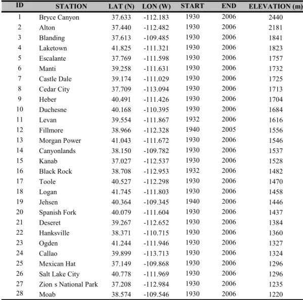
Table 1 - Meteorological stations used for the analysis of maximum and minimum daily temperature in Utah State, USA
ID STATION LAT (N) LON (W) START END ELEVATION (m)
1 Bryce Canyon 37.633 -112.183 1930 2006 2440
2 Alton 37.440 -112.482 1930 2006 2181
3 Blanding 37.613 -109.485 1930 2006 1841
4 Laketown 41.825 -111.321 1930 2006 1823
5 Escalante 37.769 -111.598 1930 2006 1757
6 Manti 39.258 -111.631 1930 2006 1732
7 Castle Dale 39.174 -111.029 1930 2006 1725
8 Cedar City 37.709 -113.094 1930 2006 1713
9 Heber 40.491 -111.426 1930 2006 1704
10 Duchesne 40.168 -110.395 1930 2006 1684
11 Levan 39.554 -111.867 1932 2006 1616
12 Fillmore 38.966 -112.328 1940 2005 1556
13 Morgan Power 41.043 -111.672 1930 2006 1546
14 Canyonlands 38.150 -109.782 1930 2006 1537
15 Kanab 37.027 -112.537 1930 2006 1528
16 Black Rock 38.708 -112.953 1932 2006 1482
17 Toole 40.527 -112.298 1930 2006 1470
18 Logan 41.745 -111.803 1930 2006 1458
19 Jehsen 40.364 -109.345 1940 2006 1446
20 Spanish Fork 40.079 -111.604 1930 2006 1437
21 Deseret 39.267 -112.652 1930 2006 1384
22 Hanksville 38.371 -110.715 1930 2006 1360
23 Ogden 41.244 -111.946 1930 2006 1327
24 Callao 39.899 -113.713 1930 2006 1324
25 Mexican Hat 37.149 -109.868 1930 2006 1296
26 Salt Lake City 40.778 -111.969 1930 2006 1296 27 Zion’s National Park 37.208 -112.984 1930 2006 1235
28 Moab 38.574 -109.546 1930 2006 1220
et al., 2006). Data Quality Control (QC) is a prerequisite for determining climatic indices. The quality control of RClimdex software performs the following procedure: 1) Replaces all missing values (currently coded as -99.9) into an internal format that the software recognizes (i.e. NA, not available), and 2) Replaces all unreasonable values into NA. Those values include daily maximum temperature less than daily minimum temperature. In addition, QC also identiies outliers in daily maximum and minimum temperature. The outliers are daily values outside a region deined by the user. Currently, this region is deined as n times standard deviation (sdt) of the value for the day, that is, (mean – n x std, mean + n x std), where std for the day and n is an input from the user (Zhang and Yang, 2004; Vincent et al., 2005). Initially, data from 50 meteorological stations were available, and after the QC, only stations with less than 10% of missing data for a period of at least 50 years were considered resulting in 28 locations (Table 1).
2.2 Methodology
Indices Name Definition Units
SU Summer Days Annual count when TX(daily maximum)>25ºC Days
ID Iced Days Annual count when TX(daily maximum)<0ºC Days TR Tropical Nights Annual count when TN(daily minimum)>20ºC Days
FD Frost days Annual count when TN(daily minimum)<0ºC Days TXx Max Tmax Monthly maximum value of daily maximum temp ºC TNx Max Tmin Monthly maximum value of daily minimum temp ºC TXn Min Tmax Monthly minimum value of daily maximum temp ºC TNn Min Tmin Monthly minimum value of daily minimum temp ºC WSDI Warm spell
duration indicator
Annual count of days with at least 6 consecutive days when TX>90th percentile
Days
CSDI Cold spell duration indicator
Annual count of days with at least 6 consecutive days when TN<10th percentile
Days
DTR Diurnal temperature range
Monthly mean difference between TX and TN ºC Table 2 - Deinition of extreme air temperature indices used in this study
Dufek and Ambrizzi, 2008). The products of the test are the statistics S and Z. A positive value of S indicates upward trend and a negative value a downward trend while Z determines the signiicance or the acceptance or rejection of the null hypothesis, H0, which states that the dataset is formed by n independent and
identically distributed random variables. When H0 is rejected at a given signiicance level, α, one can say that the dataset has a signiicant trend (Satyamurty et al, 2008). Further details can be obtained in Partal and Kahya (2006).
To run the RClimdex 1.0 software the input data ile has several requirements: 1) ASCII text ile; 2) Columns sequence: Year, Month, Day, Precipitation (PRCP), Maximum air temperature (TMAX), and Minimum air temperature (TMIN). (NOTE: PRCP units = millimeters and TMAX and TMIN units = degrees Celsius); 3) the format as described above was space delimited (e.g. each element was separated by one or more spaces); 4) for data records, missing data were coded as -99.9 (in this study the precipitation values were replaced by -99.9) and data records were in calendar date order (Zhang and Yang, 2004).
The spatial distribution of the indices trends obtained using Mann-Kendall test was represented using the symbols (Ì) for positive trends, and (●) for negative trends, statistically signiicant at 95% level, i.e. p<0.05. The representation of the trends which are statistically non-signiicant used the symbols (Æ) for positive trends, and (O) for negative trends.
3. RESULTS
Table 3 shows the decadal trends of the extreme indices of air temperature in Utah State for 28 locations. The bold and
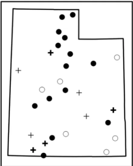
highlighted values represent signiicant level of 5% (p<0.05), and values only highlighted represent signiicant level of 10% (0.05<p<0.1). The analyses presented in this study are only those trends that showed signiicance at 5% level. The index Summer Days (SU) showed 10 stations with positive trend and 3 stations with negative trend, evidencing an increase in the annual number of days when the maximum air temperature was higher than 25ºC. The spatial distribution of the trends of this index is shown in Figure 2. The index Iced Days (ID) showed 7 stations with negative trends, 1 station with positive trend and one station (Laketown) that did not present any trend (trend = 0), showing that the annual number of days when the maximum air temperature was less than 0ºC is decreasing. These results are in agreement with the results shown by SU index. Figure 3 shows the spatial distribution trends of ID index; in general, the signiicant values are in the southern portion of the studied area. It is possible to identify the heterogeneous behavior of the indexes presenting positive and negative trends, indicating a possible inluence of local factors. These results are in agreement with those of Karl and Knight (1998).
Table 3 - Deinition of extreme air temperature indices used in this study
STATION SU ID TR FD TXx TXn TNx TNn WSDI CSDI DTR
Bryce Canyon -1.88 2.53 0 -3.33 0.14 0.39 0.20 1.21 -0.16 -0.63 -0.49 Alton 5.45 -1.25 -0.01 0.09 0.41 0.32 -0.18 0.26 1.90 -0.17 0.28 Blanding 2.84 -1.07 0.02 -2.75 0.34 0.31 0.07 0.53 2.41 -0.67 -0.03 Laketown -1.31 0.00 0 -1.94 -0.15 -0.07 0.04 0.30 -0.61 -0.30 -0.20 Escalante 4.07 -1.80 0.05 -4.41 0.52 1.03 0.31 1.04 3.75 -0.55 -0.05 Manti 0.03 0.44 0.03 -0.93 0.10 -0.13 0.24 0.47 0.54 -0.12 -0.13 Castle Dale 1.15 -3.56 0 0.22 0.27 0.87 0.10 0.84 1.99 0.02 0.21 Cedar City 0.26 -0.28 0.05 -0.51 0.19 0.37 0.11 0.65 1.20 -0.29 0 Heber 0.72 -0.19 0 -2.58 0.03 0.13 0.07 0.38 0.96 -0.33 -0.15 Duchesne 0.75 -1.22 -0.01 -3.29 0.10 0.03 0.18 0.67 0 -1.62 -0.25 Levan 0.39 0.05 0.02 0 0.28 0.08 0.01 0.41 0.21 -0.18 -0.02 Fillmore -1.74 1.46 -0.03 -2.24 -0.31 -0.28 0.01 0.32 -0.76 -0.10 -0.27 Morgan Power -0.06 -0.35 0.03 -7.32 0.26 0.38 0.47 1.13 0.75 -1.41 -0.45 Canyonlands -0.28 -1.11 3.79 -2.71 0.34 0.48 0.45 0.99 -0.13 -0.20 -0.34 Kanab 0.03 -0.14 -0.11 -2.07 -0.06 0.15 0.02 0.74 -0.51 -0.52 -0.15 Black Rock 0.20 0.36 0.04 -3.33 0.04 0.32 0.07 0.54 -0.81 -0.38 -0.23 Toole 1.68 -0.45 0.68 -0.57 0.14 0.19 0.04 0.17 1.08 0.01 0.07 Logan 0.42 -0.02 0.01 -1.04 0 0.05 -0.02 0.31 0.51 -0.60 -0.06 Jehsen 0.93 -2.35 -0.01 -1.99 0.11 0.71 0.07 0.73 0.89 -0.45 -0.13 Spanish Fork -1.34 0.77 0.08 -2.06 -0.18 0.02 0.08 0.33 -0.75 -0.66 -0.21 Deseret 0.79 0.03 0.05 -0.51 0.21 -0.06 -0.01 0.19 0 -0.62 -0.04 Hanksville 2.50 -0.67 0.31 -0.60 0.55 0.25 0.29 0.29 0.71 -0.72 0 Ogden 1.10 -0.12 0.82 -2.24 0.12 0.03 0.17 0.48 -0.03 -0.35 -0.17 Callao 5.29 -2.98 0.68 -3.40 0.73 1.08 0.64 0.54 0.51 -1.31 0.19 Mexican Hat 4.68 -2.17 4.50 -3.88 0.14 2.01 0.72 1.02 1.53 -2.51 -0.06 Salt Lake City 0.18 -0.81 1.96 -3.77 0.06 0.29 0.30 0.63 0.07 -0.87 -0.24 Zion’s N. Park 1.02 -0.06 -0.43 -1.20 0.12 0.30 -0.02 0.11 1.15 0.03 0.12 Moab 3.75 -1.95 0.88 0.08 0.57 1.01 0.13 0.96 2.96 -0.16 0.40
Figure 2 - Spatial distribution of trends of SU index to Utah State. The symbols (+), for positive trends, and (•) for negative trends, statistically
signiicant at 95% level (p<0.05), and (+) for positive trends, and (O), for negative trends (non-signiicant at 95% level).
Figure 3 - Spatial distribution of trends of ID index to Utah State. The symbols (+), for positive trends, and (•) for negative trends, statistically
positive trends and 1 station with negative trend (Figure 8). The Min Tmin (TNn) index presented a similar behavior with only positive trends (15 stations), evidencing that the minimum temperature is increasing in this region (Figure 9). The increase of the air temperature in the study area was also identiied by Karl and Knight (1998) and Alexander et al. (2007).
The Warm Spell Duration Indicator (WSDI) index, that represents the annual count of days with at least 6 consecutive days on which TX is more than the 90th percentile, showed 9 stations with positive trends and 2 stations with negative trends
Figure 5 - Spatial distribution of trends of FD index to Utah State. The symbols (+), for positive trends, and (•) for negative trends, statistically
signiicant at 95% level (p<0.05), and (+) for positive trends, and (O), for negative trends (non-signiicant at 95% level).
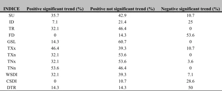
Table 4 - The percentage of stations showing signiicant and not signiicant trends at the 5% level for the temperature indices for Utah State, USA
SU 35.7 42.9 10.7
ID 7.1 21.4 25
TR 32.1 46.4 0
FD 0 14.3 53.6
GSL 14.3 60.7 0
TXx 46.4 39.3 10.7
TXn 32.1 53.6 0
TNx 32.1 53.6 3.6
TNn 53.6 46.4 0
WSDI 32.1 39.3 7.1
CSDI 0 10.7 28.6
DTR 14.3 14.3 50
INDICE Positive significant trend (%) Positive not significant trend (%) Negative significant trend (%)
stations with positive trends and 3 stations with negative trends, showing a predominant increase in the monthly maximum value of daily maximum temperature in this area (Figure 6). It is possible to observe in Min Tmax (TXn) index a similar behavior, with only positive trends (9 stations), evidencing that the monthly minimum value of daily maximum temperature is increasing as well. The spatial distribution is shown in Figure 7 and these results show an increase in the temperature in the studied area. The Max Tmin (TNx) index, i.e. monthly maximum value of daily minimum air temperature, shows 9 stations with
Figure 4 - Spatial distribution of trends of TR index to Utah State. The symbols (+), for positive trends, and (•) for negative trends, statistically
Figure 6- Spatial distribution of trends of TXx index to Utah State. The symbols (+), for positive trends, and (•) for negative trends, statistically
signiicant at 95% level (p<0.05), and (+) for positive trends, and (O), for negative trends (non-signiicant at 95% level).
Figure 7 - Spatial distribution of trends of TXn index to Utah State. The symbols (+), for positive trends, and (•) for negative trends, statistically
signiicant at 95% level (p<0.05), and (+) for positive trends, and (O), for negative trends (non-signiicant at 95% level).
Figure 8- Spatial distribution of trends of TNx index to Utah State. The symbols (+), for positive trends, and (•) for negative trends, statistically
signiicant at 95% level (p<0.05), and (+) for positive trends, and (O), for negative trends (non-signiicant at 95% level).
Figure 9 - Spatial distribution of trends of TNn index to Utah State. The symbols (+), for positive trends, and (•) for negative trends, statistically
signiicant at 95% level (p<0.05), and (+) for positive trends, and (O), for negative trends (non-signiicant at 95% level).
(Figure 10), evidencing the increase of warm spell duration. Figure 11 shows the spatial distribution of Cold Spell Duration Indicator (CSDI) index that represents the annual count of days with at least 6 consecutive days where TN is less than the 10th percentile. Table 3 shows that the CSDI index presented only negative trends (8 stations) evidencing that cold spell durations are decreasing; this result is in agreement with the result presented by the WSDI. In addition, Diurnal Temperature Range (DTR)
index shows negative trends to 14 stations and positive trends to 4 stations (Figure 12), evidencing that the monthly mean difference between maximum and minimum temperature is decreasing in the studied area. These results are in agreement with the results obtained for TXx, TXn, TNx and TNn indices. There is a similar pattern in the results obtained by Alexander et al. (2007).
stations with statistically signiicant and non-signiicant trends at the 5% level were calculated and are shown in Table 4. It is possible to see that 35.7% of the stations show a signiicant increase in SU, as well as 32.1% in TR, 46.4% in TXx, 32.1% in TXn, TNx and WSDI, and 53.6% in TNn, evidencing the increase of temperature. While there is a signiicant decrease of 25% in ID, 53.6% in FD, 28.6% in CSDI and 50% in DTR, evidencing a decrease in these indices and agreeing with the results shown previously.
The indices results, except TR, FD, TXn, TNn and CSDI, present heterogeneous behavior, i.e. positive and negative
Figure 10 - Spatial distribution of trends of WSDI index to Utah State. The symbols (+), for positive trends, and (•) for negative trends,
statistically signiicant at 95% level (p<0.05), and (+) for positive trends, and (O), for negative trends (non-signiicant at 95% level).
Figure 11 - Spatial distribution of trends of CSDI index to Utah State. The symbols (+), for positive trends, and (•) for negative trends,
statistically signiicant at 95% level (p<0.05), and (+) for positive trends, and (O), for negative trends (non-signiicant at 95% level).
Figure 12 - Spatial distribution of trends of DTR index to Utah State. The symbols (+), for positive trends, and (•) for negative trends,
statistically signiicant at 95% level (p<0.05), and (+) for positive trends, and (O), for negative trends (non-signiicant at 95% level).
signiicant trends (p<0.05), and evidencing the inluence of local factors such as urbanization and topography. For example, Laketown station has an elevation of 1.823m above sea level (only Bryce Canyon, Alton and Blanding locations have higher elevation), and presented different signal of the trends for SU, ID, TXx and WSDI indices, indicating its topography inluence.
4. CONCLUSIONS
temperatures has also decreased. These analyses identiied the temperature increase in Utah State during the last century.
5. REFERENCES
ALEXANDER, L. V., HOPE, P., COLLINS, D., TREWIN, B., LYNCH, A., NICHOLLS, N. Trends in Australia’s climate means and extremes: a global context. Australian Meteorological Magazine, v. 56, p. 1-18, 2007.
BRUNETTI, M., BUFFONI, L., MANGIANTI, F., MAUGERI, M., NANNI, T. Temperature, precipitation and extreme events during the last century in Italy. Global and Planetary Change, v. 40, p. 141–149, 2004.
BRUNETTI, M., MAUGERI, M., MONTI, F., NANNI, T. Temperature and precipitation variability in Italy in the last two centuries from homogenized instrumental time series. International Journal of Climatology, v. 26, p. 345-381, 2006.
DUFEK, A. S., AMBRIZZI, T. Precipitation variability in São Paulo State, Brazil. Theoretical and Applied Climatology, v. 93, p. 167-178, 2008.
EASTERLING, D. R., EVANS, J. L., GROISMAN, P. Y., KARL, T. R., KUNKEL, K. E. AMBENJE, P. Observed variability and trends in extreme climate events. Bulletin of American Meteorological Society, v. 81, p. 417-425, 2000. FOLLAND, C.K., KARL, T.R., CHRISTY, J.R., CLARKE,
R.A., GRUZA, G.V., JOUZEL, J., MANN, M.E., OERLEMANS, J., SALINGER, M.J. AND WANG, S.W. Observed climate variability and change. In: Climate Change 2001: The Scientiic Basis. Contribution of Working Group I to the Third Assessment Report of the Intergovernmental Panel on Climate Change. Cambridge University Press, Cambridge, UK, and New York, USA, 2001, 881 p. HAYLOCK, M. R., PETERSON, T. C., ALVES, L. M.,
AMBRIZZI, T., ANUNCIAÇÃO, Y. M. T., BAEZ, J., BARROS, V. R., BERLATO, M. A., BIDEGAIN, M., CORONEL, G., GARCIA, V. J., GRIMM, A. M., KAROLY, D., MARENGO, J. A., MARINO, M. B., MONCUNILL, D. F., NECHET, D., QUINTANA, J., REBELLO, E., RUSTICUCCI, M., SANTOS, J. L., TREBEJO, I., VINCENT, L. A. Trends in total and extreme South American rainfall 1960-2000 and links with sea surface temperature. Journal of Climate, v. 19, p. 1490-1512, 2006. INTERGOVERNMENTAL PANEL ON CLIMATE CHANGE, IPCC. Climate Change 2001 – The Scientific Basis. Contribution of Working Group I to the Third Assessment Report of the IPCC. Cambridge Univ. Press, Cambridge, 2001.
INTERGOVERNMENTAL PANEL ON CLIMATE CHANGE, IPCC. Climate Change 2007 – The Physical Science
Basis. Contribution of Working Group I to the Fourth Assessment Report of the IPCC. Cambridge Univ. Press, Cambridge, 2007.
KARL, T. R., KNIGHT, R. W. Secular trends of precipitation amount, frequency, and intensity in the USA. Bulletin of American Meteorological Society, v. 79, p. 231-241, 1998. KUNKEL, E. E., ANDSAGER, K., EASTERLING, D. R.
Long-term trends in extreme precipitation events over the Conterminous United States and Canada. Journal of Climate, v. 12, p. 2515-2527, 1999.
MOBERG, A., JONES, P. D. Trends in indices for extremes in daily temperature and precipitation in Central and Western Europe, 1901–99. International Journal of Climatology, v. 25, p. 1149-1171, 2005.
MOLLER, A. L., GILLIES, R. R. Utah Climate. Publication Design and Production: Utah State University, Logan-UT/ USA, second Edition, 2008, 115 p.
PARTAL, T., KAHYA, E. Trend analysis in Turkish precipitation data. Hydrological Processes, v. 20, p. 2011-2026, 2006. PETERSON TC, FOLLAND C, GRUZA G, HOGG W,
MOKSSIT A, PLUMMER N. Report on the activities of the working group on climate change detection and related rapporteurs 1998–2001. In World Meteorological Organization, Rep. WCDMP-47, WMO-TD 1071, Geneva, IL, 2001, 143 p.
SANTOS, C. A. C., BRITO, J. I. B. Análise dos índices de extremos para o semi-árido do Brasil e suas relações com TSM e IVDN. Revista Brasileira de Meteorologia, v. 22, p. 303-312, 2007.
SATYAMURTY, P., CASTRO, A. A., TOTA, J., GULARTE, L. E. S., MANZI, A. O. Rainfall trends in the Brazilian Amazon Basin in the past eight decades. Theoretical and Applied Climatology, 2008, DOI10.1007/s00704-009-0133-x. TORETI, A., DESIATO, F. Changes in temperature extremes
over Italy in the last 44 years. International Journal of Climatology, v. 28, p. 733-745, 2008.
VINCENT, L. A., PETERSON, T. C., BARROS, V. R., MARINO, M. B., RUSTICUCCI, M., CARRASCO, G., RAMIREZ, E., ALVES, L. M., AMBRIZZI, T., BERLATO, M. A., GRIMM, A. M., MARENGO, J. A., MOLION, L., MONCUNILL, D. F., REBELLO, E., ANUNCIAÇÃO, Y. M. T., QUINTANA, J., SANTOS, J. L., BAEZ, J., CORONEL, G., GARCIA, J., TREBEJO, I., BIDEGAIN, M., HAYLOCK, M. R., KAROLY, D. Observed trends in indices of daily temperature extremes in South America 1960–2000. Journal of Climate, v. 18, p. 5011–5023, 2005. WANG, W., CHEN, X., SHI, P., VAN GELDER, P. H. A. J. M.
ZHANG, X., HEGERL, G., ZWIERS, F. W., KENYON, J. Avoiding inhomogeneity in percentile-based indices of temperature extremes. Journal of Climate, v. 18, p. 1641–1651, 2005.