www.biogeosciences.net/10/8363/2013/ doi:10.5194/bg-10-8363-2013
© Author(s) 2013. CC Attribution 3.0 License.
Biogeosciences
Technical Note: The effect of vertical turbulent mixing on gross O
2
production assessments by the triple isotopic composition of
dissolved O
2
E. Wurgaft, O. Shamir, and A. Angert
The Freddy and Nadine Herrmann Institute of Earth Sciences, The Hebrew University of Jerusalem, Jerusalem, Israel
Correspondence to:E. Wurgaft ([email protected])
Received: 19 August 2013 – Published in Biogeosciences Discuss.: 27 August 2013
Revised: 15 November 2013 – Accepted: 20 November 2013 – Published: 20 December 2013
Abstract.The 17O excess (171)of dissolved O2 has been used, for over a decade, to estimate gross O2 production (G17OP) rates in the mixed layer (ML) in many regions of the ocean. This estimate relies on a steady-state balance of O2fluxes, which include air–sea gas exchange, photosynthe-sis and respiration but notably, not turbulent mixing with O2 from the thermocline. In light of recent publications, which showed that neglecting the turbulent flux of O2 from the thermocline may lead to inaccurate G17OP estimations, we present a simple correction for the effect of this flux on ML G17OP. The correction is based on a turbulent-flux term tween the thermocline and the ML, and use the difference be-tween the ML171and that of a single data-point below the ML base. Using a numerical model and measured data we compared turbulence-corrected G17OP rates to those calcu-lated without it, and tested the sensitivity of the GOP correc-tion for turbulent flux of O2from the thermocline to several parameters. The main source of uncertainty on the correction is the eddy-diffusivity coefficient, which induces an uncer-tainty of∼50 %. The corrected G17OP rates were 10–90 % lower than the previously published uncorrected rates, which implies that a large fraction of the photosynthetic O2in the ML is actually produced in the thermocline.
1 Introduction
Gross O2 production (GOP) in the ocean is a fundamental process in the global cycling of O2. As such, accurate es-timates of GOP rates are essential in order to understand and model the global cycles of oxygen and carbon. During
the past decade, the application of the triple isotope compo-sition (16O,17O, and 18O) of dissolved O2 as a tracer for GOP (G17OP), which was first presented by Luz and Barkan (2000), has become widespread and has been used to esti-mate GOP rates in many regions of the ocean (Juranek and Quay, 2013, and refs. within).
1.1 GOP from171
Estimating GOP rates from the isotopic composition of dis-solved O2 is based on the17O-excess (171)that photosyn-thetically produced O2has in comparison to atmospheric O2 (Luz et al., 1999). The171has been defined in several ways (Kaiser, 2011). A common definition (Miller, 2002; Luz and Barkan, 2005), which we use here is
171=
ln(δ17O+1)−λln(δ18O+1), (1) whereδ*O =(∗R
sample/∗Rref – 1); ∗Rsample and ∗Rref are the *O/16O in the sample and the reference, respectively.
λ is the slope of a reference line on a ln(δ17O+1) versus ln(δ18O+1) plot, which represents the expected slope of the relevant processes. Following Luz and Barkan (2005), most studies useλ=0.518 for the calculation of 171and atmo-spheric O2as a standard for the isotopic measurements. To derive a steady-state expression for GOP in the mixed layer (ML), Luz and Barkan (2000) used an O2 and 1711-box model. Their derivation yielded the following equation: G17OP=K (O2)eq
171
dis−171eq 171
p−171dis
, (2)
the 171value of dissolved O2,171eq the equilibrium171 with respect to atmospheric O2, and 171p 171 at steady state between photosynthesis and respiration. Recently, Luz and Barkan (2000) method for ML GOP estimation (here-after G17OPLB)was revised by Prokopenko et al. (2011) and Kaiser (2011), who derived equations for G17OP that use measured δ17O andδ18O, the isotopic composition of dis-solved O2in air–seawater equilibrium (δ17Oeqandδ18Oeq), and the isotopic composition of photosynthetic O2 (δ17Op andδ18Op). Unlike Eq. (2), their equations avoided a num-ber of numerical approximations. They did, however, rely onδ17Opandδ17Oeqwhich are still subject to disagreement among researchers in the field (e.g. Kaiser and Abe, 2012). However, Luz and Barkan (2011a, b) and Nicholson (2011) showed that if properδ17Opandδ18Opare assigned, the dif-ferences between G17OPLBand the G17OP estimated by the revised versions are small.
1.2 The effect of turbulent mixing on G17OP estimation
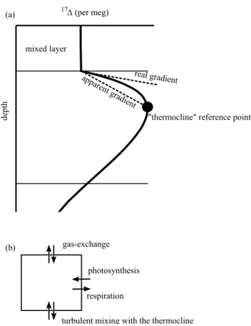
As in Luz and Barkan (2000), the ML G17OP equa-tions that were presented by Prokopenko et al. (2011) and Kaiser (2011) were derived with a 1-box representation of the ML in which a steady-state balance exists between the O2fluxes of GOP, respiration and air–sea gas exchange, but without accounting for the flux of turbulent mixing with O2 from the thermocline. This was, in spite of the fact that ver-tical171profiles often show a pronounced increase below the ML base (Fig. 1; Luz and Barkan, 2000; Juranek and Quay, 2005; Quay et al., 2010). Juranek and Quay (2005) estimated that vertical turbulence had a negligible affect over G17OP. However, Nicholson et al. (2012) showed that mix-ing of ML O2with high171O2 from the thermocline into the ML (by either entrainment due to ML deepening, or by turbulent flux) may result in an overestimation of up to 80 % in ML G17OP. Nicholson et al. (2012) further suggested that this overestimation was the likely explanation for the higher ratio of G17OP to14C-based net primary productivity (G17OP : NPP(14C); Marra, 2002; Juranek and Quay, 2005; Quay et al., 2010), compared to the ratio of GOP estimated from18O incubations to the same net productivity estimate (G18OP : NPP(14C)). In addition, Jonsson et al. (2013) found that the turbulent mixing had a considerable effect on estima-tion of net O2production, using O2: Ar measurements.
As noted above, high171O2 from the thermocline can mix into the ML either by entrainment of water from the thermocline into the ML, which takes place as the ML base deepens, or by vertical turbulence of O2 from the thermo-cline. The latter process dominates when the ML depth is constant (Fig. 1). Nicholson et al. (2012) did not consider these two process separately; however, their findings showed that G17OP overestimated GOP even when the ML depth was relatively constant, which indicates that vertical turbulence also affects G17OP.
real gradient appa
rent gr adient
de
pt
h
mixed layer
"thermocline" reference point
gas-exchange
photosynthesis
respiration
turbulent mixing with the thermocline (a)
(b)
17Δ (per meg)
Fig. 1. (a)A schematic illustration of a typical mid-ocean171 ver-tical profile. The dashed lines, which extend below the mixed-layer base define the171gradient, which in turn, is correlated with the 171“flux” into the mixed layer. Depending on the profile shape, the choice of a “thermocline“ reference point at some depth below the mixed-layer depth, results in a171gradient which is different than the real171gradient.(b)A conceptual model of the O2 iso-topologues fluxes in and out of the ML.
While Sarma et al. (2006) and Quay et al. (2010) discussed the effect of entrainment on G17OP and suggested non-steady-state corrections, and Castro-Morales et al. (2012) suggested a correction for the vertical flux of O2into the ML, the effect of turbulence on the triple isotopic composition and the resulting effect on ML G17OP estimations has not been explicitly examined. In light of Nicholson et al. (2012) and Jonsson et al. (2013) results, it is clear that to accurately esti-mate G17OP rates, the magnitude of the turbulent mixing ef-fect should be evaluated, and if large, corrected for. The aims of this work were to evaluate the magnitude of the effect of turbulent mixing on ML G17OP estimation, and to derive an analytical correction for this effect.
2 Derivation of a GOP equation with a turbulent mixing term
derivation of time variations of O2isotopologues. We added a turbulent-flux term to Eq. (4) and Eq. (5) in Prokopenko et al. (2011). The turbulent flux was calculated between the base of the ML and a single point along the171 gradient below the ML, which was assigned as “thermocline” (Fig. 1). Consequently, the171gradient below the ML was assumed to be linear with depth (we will revisit this assumption in sensitivity tests section). The resulting equation for the rate of change in171in the ML was (full derivation of the equa-tion can be found in Appendix A):
h (O2)∂
171
∂t =G17OPC
X17 p−X17
X17
−λ
X18 p−X18
X18
−K (O2)eq
X17−X17 eq
X17
−λ
X18−X18 eq
X18
− κ
Z(O2)thr
X17−X17 thr
X17
−λ
X18−X18 thr
X18
(3)
wherehis the ML depth, (O2) is the dissolved O2 concen-tration in the ML,κ is the eddy-diffusivity coefficient, and
Z is the vertical distance between the base of the ML and the depth assigned as “thermocline”. For convenience, we useD=κ/Zhereafter. X∗represents the ratio∗O/16O. The subscripts “p” and “eq” denote “photosynthetic” and “equi-librium”, respectively. Note that as was shown by Luz and Barkan (2009) and Prokopenko et al. (2011), the rate of change of171is independent of respiration. When steady-state conditions in the ML are assumed, the resulting term for turbulent-flux corrected G17OP is
G17OPC=K (O2)eq
X17−X17eq X17
−λ
X18−X18eq
X18
X17p −X17
X17
−λ
X18p −X18 X18
+D (O2)thr
X17−X17 thr X17
−λ
X18−X18
thr X18
X17p−X17
X17
−λ
X18p −X18 X18
,
(4)
where G17OPCis the G17OP corrected for turbulent flux of O2from the thermocline. For convenience we will abbreviate the GOP correction for turbulent flux of O2from the thermo-cline (the second term on the right-hand side in Eq. 4) to “TFC” hereafter. The numerator of the TFC represents the contribution of the turbulent flux to the GOP estimated from 171in the ML.
3 Simulations by a 1-D numerical model
We used a simple 1-D model, which simulated the ef-fects of GOP, respiration, gas exchange and turbulence on each O2isotopologue, to compare the G17OP rates obtained by Eq. (4) with those obtained without applying the TFC. Briefly, the model simulated the water column up to a depth of 300 m, which was divided into 30 layers of 10 m each, and calculated the fluxes of each O2 isotopologue in each layer produced by photosynthesis, respiration, and turbulent
60
70
80
90
100
110
0
10
20
30
40
50
60
y= 0.9x-52
R
2=0.9998
GO
P ove
r e
st
im
at
ion (
%
)
17
Δ below the mixed layer (per meg)
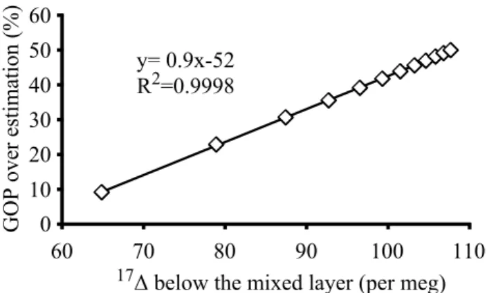
Fig. 2. Linear regression analysis of model simulation re-sults, showing the increase in mixed-layer GOP overestimation ((G17OPPRO/GOPM−1)·100) versus171below the mixed layer.
mixing (model equations, parameters and MATLAB files are given in the Supplement). An additional layer at the top of the water column represented the ocean surface. In this layer, (O2) and its isotopic composition were kept in air– sea equilibrium. The eddy-diffusivity coefficient in the ML (2.5×10⁻³m2s−1)was assigned so as to let (O2) in the ML be fully mixed. The concentration of each isotopologue in the ML was affected by turbulent mixing with the upper-most layer, photosynthesis, respiration and turbulent mixing with the seasonal thermocline residing below. For the sea-sonal thermocline, we usedκ=10−4m2s−1(see sensitivity tests section).
We ran two simulations to examine the effect of turbulent mixing on ML G17OP. In the “fixed mixing depth” simula-tion (Table 1) we ran the model with a constant ML depth of 40 m. The layer directly below the ML base, at 50 m, was assigned as the “thermocline” data point for TFC calcula-tion. MLδ17O,δ18O and171values were calculated every 30 model time steps (model month). In the first model month of the simulation, G17OPLBand G17OPPROslightly overes-timated (by 7 %) the GOP assigned in the model (GOPM). In the following model months, the overestimation of both G17OPLB and G17OPPRO increased, reaching ∼40 % after 5 model months. As shown in Fig. 2, the increase in GOP overestimation was closely related to the increase in 171
in the seasonal thermocline. However, G17OPC, which cor-rects for the turbulent mixing flux of O2 from the thermo-cline, remained constant with a slight underestimation of ∼7 % throughout the entire simulation period. When we ef-fectively shut down turbulent mixing in the model by re-ducingκ within the thermocline to 10−6m2s−1, G17OP
LB and G17OPPRO were in good agreement with GOPM. This indicates that turbulent flux was indeed the cause of the overestimation.
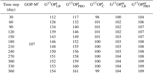
Table 1. Results of model simulation with a constant mixed-layer depth of 40 m GOP-M – input GOP rate, G17OPLB – Luz and Barkan (2000), G17OPPRO– Prokopenko et al. (2011), G17OPC– this work includes a correction for turbulent flux of O2from the thermo-cline. All GOP rates are in mmol m−2day−1. In the columns marked with t,κ=10−4m2s−1, whereas in the columns marked with nt,κ= 10−6m2s−1, which effectively shuts down the turbulent flux of O
2between the thermocline and the mixed layer. Time step GOP-Mt G17OPtLB G17OPtPRO G17OPtC G17OPntLB G17OPntPRO
(day)
30
107
112 117 98 100 104
60 126 132 101 102 106
90 134 140 101 102 107
120 139 146 101 102 107
150 143 149 101 103 107
180 146 152 100 103 108
210 148 155 100 103 108
240 150 156 100 103 108
270 151 158 100 104 108
300 152 159 100 104 109
330 153 160 100 104 109
360 154 161 99 104 109
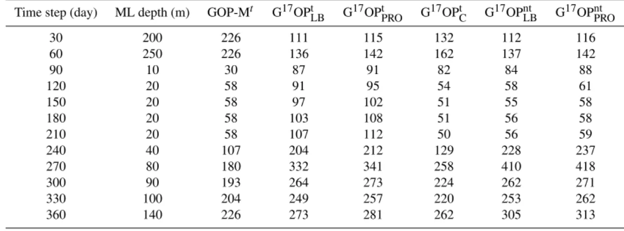
ML depth underwent rapid changes (in the model months corresponding to January–March and August–December in BATS), the steady-state assumption was not valid, and nei-ther G17OPLB and G17OPPRO, nor G17OPC yielded GOP rates comparable to GOPM. On the other hand, when the ML depth experienced small variations (in the months when ML depth corresponded to April–August in BATS), G17OPC rates were close to GOPM, while G17OPLBand G17OPPRO were about 60–90 % greater than GOPM.
4 Sensitivity tests
In addition to simulating the effect of turbulent mixing on GOP estimations, we used the 1-D model to test the sensi-tivity of the TFC to the depth of the “thermocline” reference point, to the analytical error associated with171 measure-ments, and to the ML depth.
The choice of the depth which represents the “thermo-cline” point can affect the resulting GOP (Fig. 1). While the TFC assumes a linear171gradient between the ML and the “thermocline”, the actual171gradient is not necessarily so. Therefore, the closer the “thermocline” point to the ML base, the better it represents the actual fluxes of O2isotopolouges between the ML and the thermocline (Fig. 1). On the other hand, the difference in the isotopic composition between the ML and the “thermocline” has to be considerably larger than the analytical error associated with171measurements (∼7 per meg; e.g. Reuer et al., 2007). In order to assess the sensi-tivity of the TFC to the depth of the “thermocline” reference point and to the analytical error on171, we calculated the magnitude of the turbulence correction with different “ther-mocline” reference points. As illustrated in Fig. 3a, the mag-nitude of the TFC decreased as the distance between the ML
base and the “thermocline” reference point increased. As-suming that the TFC calculated using the “thermocline” im-mediately (10 m) below the ML is the most accurate, we con-sider the difference between this value and the TFC calcu-lated for other “thermocline” depths as the error induced on the TFC by the selection of the “thermocline” depth. Using the same 1-D model simulations, we calculated the effect of the analytical error associated with171measurements on the magnitude of the TFC. For this end, we calculated the TFC three times per each “thermocline” depth. The first TFC was calculated without error on171values, whereas for the other two, a 7 per meg error was either added or subtracted from the171values of the ML and the “thermocline”. The com-binations which yielded the maximal deviations from the no-error TFC are illustrated by the vertical no-error bars in Fig. 3a. The magnitude of this error decreased with increasing depth of the “thermocline”. Finally, we estimated the combined ef-fect of the choice of the “thermocline” depth and the ana-lytical error on the TFC, by propagating these two errors. The resulting error is illustrated in Fig. 3a. For the scenario used in our tests, the minimal error (∼20 %) was observed at 20 m below the ML base. We note that this error is likely to be an overestimation of the actual error which results from these two factors, since we used the maximal analytical er-ror on both ML171and171thrvalues simultaneously, and in reverse directions, which yielded the maximal effect on the resulting171gradient. Moreover, as the ML171value is usually an average of several measurements, it is likely to be subject to a much smaller error than 7 per meg.
Table 2.Results of model simulation of GOP with varying mixed-layer depth ML – mixed layer, GOP-M – input GOP rate, G17OPLB– Luz and Barkan (2000), G17OPPRO– Prokopenko et al. (2011), G17OPC– this work includes a correction for turbulent flux of O2from the thermocline. All GOP rates are in mmol m−2day−1. In the columns marked with t,κ=10−4m2s−1, whereas in the columns marked with nt,κ=10−6m2s−1, which effectively shuts down the turbulent flux of O
2between the thermocline and the mixed layer. Time step (day) ML depth (m) GOP-Mt G17OPtLB G17OPtPRO G17OPtC G17OPntLB G17OPntPRO
30 200 226 111 115 132 112 116
60 250 226 136 142 162 137 142
90 10 30 87 91 82 84 88
120 20 58 91 95 54 58 61
150 20 58 97 102 51 55 58
180 20 58 103 108 51 56 58
210 20 58 107 112 50 56 59
240 40 107 204 212 129 228 237
270 80 180 332 341 258 410 418
300 90 193 264 273 224 262 271
330 100 204 249 257 220 253 262
360 140 226 273 281 262 305 313
Depth of the “Thermocline” ref. point below ML base (m)
ML depth (m)
(m
m
ol
O2
m
-2da
y
-1)
(m
m
ol
O2
m
-2da
y
-1)
(%)
0 10 20 30 40 50 60 70
-70 -60 -50 -40 -30 -20 -10 0
0 20 40 60 80 120 140
0 10 20 30 40 50 60 70 80
TFC Error on TFC
100
0 20 40 60 80 100 120 140
TFC
Er
ror
on T
FC
Tur
bul
ent
fl
ux c
ont
ribut
ion t
o GO
P
Fig. 3.Sensitivity of the turbulent-flux correction.(a)The sensitiv-ity of the GOP correction for turbulent flux of O2from the thermo-cline (TFC) to the depth of the “thermothermo-cline” reference point below the mixed layer (ML). The error bars represent the maximal error on the TFC, induced by the analytical error associated with171 mea-surements (7 per meg). The error resulting from the combination of these two factors (circles) on the TFC shows a minimum at 20 m below ML.(b)The relative contribution of turbulent mixing flux to estimated G17OP as a function of the ML depth. Model conditions for each sensitivity test are described in Sect. 4 in the text.
values in the thermocline approached maximal values (∼250 per meg), whereas observed summer values in the thermo-cline do not exceed 160 per meg (Juranek and Quay, 2005, Quay et al., 2010) in the Hawaii Ocean time-series (HOT) station and similar values in Bermuda Atlantic time-series
(BATS) station (Nicholoson et al., 2011). Moreover, Nichol-son et al. (2012) used similar values (8–9×10⁻⁵m2s−1) to reproduce the physical conditions (ML depth, heat con-tent and sea surface temperature) in the upper 1000 m in the BATS and in HOT. Therefore, we estimate that our choice of
κ was rather accurate for the processes of turbulent mixing between the ML and the seasonal thermocline. Apparently, in spite of the fact that 1×10⁻⁴m2s−1is almost an order of magnitude higher than the value estimated from SF6release experiments in the permanent thermocline (∼300 m, Led-well et al., 1993),κvalues near the interface between the ML and the thermocline are higher than those which characterize the thermocline at greater depths where SF6release experi-ments were conducted. Given the highly unrealistic profiles we obtained for lower values and the agreement between our model and the model used by Nicholson et al. (2012), we assume an uncertainty of∼50 % on this value, and conse-quently, a 50 % uncertainty on the TFC term.
Finally, we tested the sensitivity of the TFC to the ML depth. The results (Fig. 3b) show that as the ML depth in-creases, the contribution of turbulence to the uncorrected GOP decreases. This implies that correcting G17OP rates for turbulent fluxes of O2isotopologues from the thermocline is especially important in ocean areas in which the summer ML is relatively shallow, such as in BATS.
5 The effect of turbulent mixing on measured GOP rates
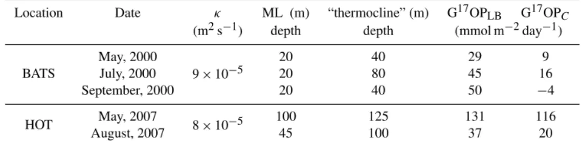
and G17OPCin Hawaii Ocean time series (HOT). To use the TFC, we chose months in which vertical profiles of171and O2were measured and published (Nicholson et al., 2012). Following our conclusions from the 1-D model simulations, we compared months in which there were no major changes in ML depth. Theκ values for BATS and HOT were both taken from Nicholson et al. (2012).
ML depth was determined as the depth in which a differ-ence of 0.5 % in O2concentration relative to the sea surface was observed (Castro-Morales and Kaiser, 2012). The “ther-mocline” reference point was assigned as the depth nearest to the ML base in which171was at least 14 per meg larger than 171in the ML. In BATS,Kvalues were obtained from Luz and Barkan (2009). In HOT, wind speed data from∼10 days before the cruise were obtained from QuickScat database, andKwas estimated according to Sweeney et al. (2007). The results (Table 3) showed that G17OPCrates were 65–100 % lower than G17OPLBin BATS, and 10–40 % lower in HOT. These results are in agreement with Nicholson et al. (2012), who estimated the effect of mixing as 60–90 % of G17OP. We note that Luz and Barkan (2009) used Wanninkhof (1992) parameterization forKin BATS. Applying more recent pa-rameterization (Ho et al., 2006; Sweeny et al., 2007), which gives lower estimates of gas-exchange rates, would result in an even greater contribution of the O2turbulent flux from the thermocline.
6 Discussion
Our results showed that vertical turbulence of O2 from the thermocline, affects ML G17OP estimations, such that cor-rected G17OP rates are considerably lower than the uncor-rected rates. This indicates that a large fraction of the ML photosynthetic O2is not produced in the ML itself, but rather in the thermocline below it. However, our results also show that the turbulent contribution to the ML 171 can be cor-rected in a rather simple manner. While the correction it-self was derived using several approximations, such as con-stant ML depth, and concon-stant 171 gradient between the thermocline and the ML, most of the resulting uncertain-ties also exist in the uncorrected equations for G17OP (Luz and Barkan 2000, Prokopenko et al., 2010). These uncer-tainties are intrinsic to any extrapolation in time and space of GOP rates estimations from a “snap-shot” profile. More-over, our sensitivity tests showed that the uncertainty on the TFC is smaller than 50 %, and therefore, we concluded that in spite of the approximations and uncertainties involved, using the TFC will improve the accuracy of G17OP esti-mations. Below, we discuss the technical aspects and the implications of these findings.
6.1 Applying GOP correction for turbulent
flux of O2from the thermocline in oceanographic measurements
Our results showed that when the ML depth does not change considerably, the effect of turbulent flux on ML GOP esti-mation can be corrected. However, to apply the correction, at least one point of data, which includes [O2] and its iso-topic composition below the ML is necessary. Such data points are easy to obtain in time-series study sites, such as BATS and HOT, but can complicate basin-wide G17OP esti-mations, which usually rely on underway seawater systems installed on ships of opportunity for sampling (Juranek and Quay, 2010; Juranek et al., 2012). In the future, such studies would need to either collect several representative “thermo-cline” samples from the thermocline along the cruise route, or use existing data if available to apply the TFC. Such cor-rections could also be applied to existing data.
The TFC is sensitive to the exact depth of the “thermo-cline” data point (Fig. 3a), and to the analytical error on171
measurements. Technical improvements which would reduce the error on171measurements would also increase the ac-curacy of G17OP estimations in general, and the accuracy of the TFC in particular. As shown in Fig. 3a, the error induced on the TFC by the analytical error, decreases with the depth selected for the “thermocline”, while the error induced by deviation of the171profile from a linear one increases with depth. In the depth range immediately below the ML base, these effects cancel each other to some extent, and an opti-mal depth can be estimated. This depth is dependent on the vertical distribution of171in each study-site, and on the an-alytical error associated with the171measurement process applied. In practical terms, we suggest using the minimum depth in which the171value is significantly (within the an-alytical uncertainty) different than the ML value.
Previous knowledge of 171 dynamics for the study site would help with choosing the optimal depth to col-lect the “thermocline” sample. For example, Juranek and Quay (2005) and Quay et al. (2010) have shown that dur-ing summer months in HOT, differences greater than 60 per meg (an order of magnitude higher than the analytical error) between the ML and thermocline171could be found within 20–40 m below the ML base. In BATS,171gradients tend to be smaller, and a difference of 60 per meg can usually be found 40–60 m below the ML depth (Nicholson et al., 2012). Therefore, the “thermocline” optimal depth is likely to be shallower in HOT than in BATS, and consequently, associ-ated with a smaller error.
6.2 Parameterization of gas exchange and eddy diffusivity
Table 3.Comparison of G17OP rates from BATS and HOT ML – mixed layer, G17OPLB– Luz and Barkan (2000), “thermocline” – depth of the data point representing the thermocline. G17OPC– G17OP corrected for turbulent flux of O2from the thermocline. All the parameters used for the calculations made in BATS were taken from Luz and Barkan (2009).κ values and the raw data used for the calculation of G17OPLBand G17OPC, and the parameters used for the calculations in HOT were taken from Nicholson et al. (2012). ML depth was determined as the depth in which a difference of 0.5 % in O2concentration relative to the sea surface was observed. Gas-exchange rates in HOT were calculated according to Sweeney et al. (2007) from wind speed data obtained from QuickSCAT.
Location Date κ ML (m) “thermocline” (m) G17OPLB G17OPC
(m2s−1) depth depth (mmol m−2day−1)
BATS
May, 2000
9×10⁻⁵
20 40 29 9
July, 2000 20 80 45 16
September, 2000 20 40 50 −4
HOT May, 2007 8×10⁻⁵ 100 125 131 116
August, 2007 45 100 37 20
κ may yield inaccurate G17OPC rates. We assume that the negative G17OPCrate that we obtained in BATS in Septem-ber 2000 (Table 3) was the result of inaccurate choice ofK
and κ. We also acknowledge the fact that the uncertainty onκ is the largest source of error on the magnitude of the TFC. Since the main aims of this work were to show the im-portance of turbulence effects and to suggest a correction, rather than to perform accurate GOP estimations, we used crude estimations ofKandκ. However, the fact that171in the ML depends upon GOP, gas-exchange and turbulent flux from the thermocline, means that in future studies any one of these three parameters could be estimated by performing simultaneous measurements of the other two parameters. For example, if GOP is estimated by18O incubations and gas exchange is estimated from wind speed measurements,171
profiles could be used to estimateκ in the seasonal thermo-cline. Moreover, since 18O incubations are not affected by turbulence, it is likely that provided that K and κ are ac-curately parameterized, G17OPC: N14CP would agree with G18OP : N14CP (Marra, 2002).
7 Conclusions
1. Turbulent fluxes of O2isotopologues from the thermo-cline have a pronounced effect over171values in the ML, and consequently, over the accuracy of G17OP es-timations.
2. An accurate G17OP estimate can be obtained by us-ing a simple correction for the effect of the turbulent fluxes.
3. The main source of uncertainty on the GOP correc-tion for turbulent flux of O2from the thermocline is the eddy-diffusivity coefficient, which causes∼50 % uncertainty.
4. The GOP correction for turbulent flux of O2from the thermocline is applicable when the mixed-layer depth
does not change sharply, and requires measurements of O2and its isotopic composition in a single point below the mixed layer, in addition to the standard measure-ments of these values in the mixed layer.
Appendix A
Derivation of the term for correcting mixed-layer gross O2production to turbulent flux of O2from the
thermocline
Like Prokopenko et al. (2011), we consider a surface mixed-layer subject to respiration, photosynthesis and gas exchange with the atmosphere, but which also exchanges water with the underlying “thermocline” layer via turbulent diffusion. In the current box model framework, we parameterize the turbulent O2flux with the “thermocline“ layer as
−κ
Z((O2)−(O2)thr) , (A1)
where (O2) and (O2)thrare the dissolved O2concentrations in the mixed layer and in the thermocline, respectively.κ is the eddy diffusion coefficient andZ is the vertical distance between the base of the ML and the depth assigned as “ther-mocline”. For convenience, we useD=κ/Zhereafter. Like-wise, turbulent fluxes of O2isotopes are parameterized as
−D (O2)X∗−(O2)thrX∗thr
, (A2)
where X∗
represents the ratio∗
O/16O. The mass balances for O2and its isotopes are given by
h∂((O2))
∂t =GOP−R−K (O2)−(O2)eq
−D ((O2)−(O2)thr, )
(A3)
h∂((O2)X∗)
∂t =GOPX
∗
p−Rα∗X∗−K
(O2)X∗−(O2)eqX∗eq
wherehis the mixed-layer depth,tis time, GOP is the gross O2production,Ris the respiration rate andKis the piston velocity.α∗
is the fractionation factor associated with res-piration for each isotopologue. The subscripts “p” and “eq” denote “photosynthetic” and “equilibrium”, respectively.
The remainder of the derivation is carried out by straight-forward applications of the steps outlined in Prokopenko et al. (2011), and repeated here for the sake of completion. The left-hand side of Eq. (A4) can be written explicitly as
h∂((O2)X∗) ∂t =hX
∗∂((O2))
∂t +h (O2) ∂(X∗)
∂t . (A5)
Upon substituting the left-hand side, and the first term on the right-hand side of Eq. (A3) with Eq. (A4) and Eq. (A3), respectively, rearranging and dividing by X∗
one gets
h (O2)X1∗ ∂(X∗)
∂t =GOP X∗
p−X ∗
X∗
+R (1−α∗)
+K (O2)eq X∗
eq−X∗ X∗
+ +D (O2)thr X∗
thr−X ∗
X∗
. (A6)
Note that the left-hand side of Eq. (A6) is equal to
h (O2)∂(ln X
∗)
∂t . On the other hand,
17O excess is defined as
171
=ln(δ17O+1)−λln(δ18O+1). (A7) Taking the derivative of Eq. (A7) with respect to time and multiplying byh (O2)yields
h (O2)
∂ 171
∂t =h (O2)
∂ ln X17
∂t −λ
∂ ln X18
∂t
!
. (A8)
Substituting Eq. (A6) into Eq. (A8) yields
h (O2)∂
171
∂t =G17OPC
X17p−X17
X17
−λ
X18p−X18
X18
−K (O2)eq
X17−X17eq
X17
−λ
X18−X18eq
X18
−D (O2)thr
X17−X17thr X17
−λ
X18−X18thr X18
,
(A9)
where G17OPC is the turbulence-corrected G17OP. Note, the respiration term is not affected by the addition of the turbulent-flux term and is cancelled out in the expression for the changes in17O excess, as expected.
Finally, for a mixed layer in steady state, we obtain the fol-lowing expression for GOP corrected for turbulent diffusion:
G17OPC= K (O2)eq
X17−X17eq X17
−λ
X18−X18eq
X18
X17p −X17
X17
−λ
X18p−X18 X18
+D (O2)thr
X17−X17 thr X17
−λ
X18−X18
thr X18
X17p−X17
X17
−λ
X18p −X18 X18
.
(A10)
Supplementary material related to this article is available online at http://www.biogeosciences.net/10/ 8363/2013/bg-10-8363-2013-supplement.zip.
Acknowledgements. We acknowledge B. Luz and N. Paldor for their useful advice and support. B. Lazar, H. Gildor and J. Erez also provided many helpful ideas. A. Gross kindly read and commented on the manuscript. The manuscript benefited from the constructive remarks of two anonymous reviewers. We are thankful for that. This research was supported by the Levi Eshkol Fellowship from the Israeli Ministry of Science and Technology, by the Harry and Sylvia Hoffman Leadership and Responsibility Fellowship and by GIF grant 1139/2011.
Edited by: K. Suzuki
References
Castro-Morales, K., Cassar, N., Shoosmith, D. R., and Kaiser, J.: Biological production in the Bellingshausen Sea from oxygen-to-argon ratios and oxygen triple isotopes, Biogeosciences, 10, 2273–2291, doi:10.5194/bg-10-2273-2013, 2012a.
Castro-Morales, K. and Kaiser, J.: Using dissolved oxygen concen-trations to determine mixed layer depths in the Bellingshausen Sea, Ocean Sci., 8, 1–10, doi:10.5194/os-8-1-2012, 2012b. Ho, D. T., Law, C. S., Smith, M. J., Schlosser, P., Harvey,
M., and Hill, P.: Measurements of air-sea gas exchange at high wind speeds in the Southern Ocean: Implications for global parameterizations, Geophys. Res. Lett., 33, L16611, doi:10.1029/2006GL026817, 2006.
Jonsson, B. F., Doney, S. C., Dunne, J., and Bender, M.: Eval-uation of Southern Ocean O2/Ar based NCP estimates in a model framework, J. Geophys. Res.-Biogeo., 118, 385–399, doi:10.1002/jgrg.20032, 2013.
Juranek, L. W. and Quay, P. D.: In vitro and in situ gross primary and net community production in the North Pacific Subtropical Gyre using labeled and natural abundance iso-topes of dissolved O2, Global Biogeochem. Cy., 19, Gb3009, doi:10.1029/2004gb002384, 2005.
Juranek, L. W. and Quay, P. D.: Basin-wide photosynthetic production rates in the subtropical and tropical Pacific
Ocean determined from dissolved oxygen isotope
ra-tio measurements, Global Biogeochem. Cy., 24, Gb2006, doi:10.1029/2009gb003492, 2010.
Juranek, L. W., Quay, P. D., Feely, R. A., Lockwood, D., Karl, D. M., and Church, M. J.: Biological production in the NE Pa-cific and its influence on air-sea CO2flux: Evidence from dis-solved oxygen isotopes and O2/Ar, J. Geophys. Res.-Oceans, 117, C05022, doi:10.1029/2011jc007450, 2012.
Juranek, L. W. and Quay, P. D.: Using triple isotopes of dissolved oxygen to evaluate global marine productivity, Ann. Rev. Mar. Sci., 5, 503–524, doi:10.1146/annurev-marine-121211-172430, 2013.
Kaiser, J. and Abe, O.: Reply to Nicholson’s comment on “Consis-tent calculation of aquatic gross production from oxygen triple isotope measurements” by Kaiser (2011), Biogeosciences, 9, 2921–2933, doi:10.5194/bg-9-2921-2012, 2012.
Ledwell, J. R., Watson, A. J., and Law, C. S.: Evidence for slow mixing across the pycnocline from an open-ocean tracer-release, Nature, 364, 701–703, doi:10.1038/364701a0, 1993.
Luz, B., Barkan, E., Bender, M. L., Thiemens, M. H., and Boer-ing, K. A.: Triple-isotope composition of atmospheric oxygen as a tracer of biosphere productivity, Nature, 400, 547–550, doi:10.1038/22987, 1999.
Luz, B. and Barkan, E.: Assessment of oceanic productivity with the triple-isotope composition of dissolved oxygen, Science, 288, 2028–2031, doi:10.1126/science.288.5473.2028, 2000. Luz, B. and Barkan, E.: The isotopic ratios 17O/16O and
18O/16O in molecular oxygen and their significance in bio-geochemistry, Geochim. Cosmochim. Ac., 69, 1099–1110, doi:10.1016/j.gca.2004.09.001, 2005.
Luz, B. and Barkan, E.: Net and gross oxygen production from O2/Ar,17O/16O and18O/16O ratios, Aqut. Microb. Ecology, 56, 133–145, doi:10.3354/ame01296, 2009.
Luz, B. and Barkan, E.: Oxygen isotope fractionation in the ocean surface and17O/16O of atmospheric O2, Global Biogeochem. Cy., 25, Gb4006, doi:10.1029/2011gb004178, 2011a.
Luz, B. and Barkan, E.: Proper estimation of marine gross O2 pro-duction with17O/16O and18O/16O ratios of dissolved O2, Geo-phys. Res. Lett., 38, L19606, doi:10.1029/2011gl049138, 2011b. Marra, J.: Approaches to the measurement of plankton production, in: Phytoplankton productivity: carbon assimilation in marine and freshwater ecosystems, edited by: Williams, P. J., Thomas, D. N., and Reynolds, R. C., Blackwell Science, Malden, MA, 78–108, 2002.
Miller, M. F.: Isotopic fractionation and the quantification of17O anomalies in the oxygen three-isotope system: an appraisal and geochemical significance, Geochim. Cosmochim. Ac., 66, 1881– 1889, doi:10.1016/s0016-7037(02)00832-3, 2002.
Nicholson, D. P.: Comment on: “Technical note: Consistent calcula-tion of aquatic gross produccalcula-tion from oxygen triple isotope mea-surements” by Kaiser (2011), Biogeosciences, 8, 2993–2997, doi:10.5194/bg-8-2993-2011, 2011.
Nicholson, D. P., Stanley, R. H. R., Barkan, E., Karl, D. M., Luz, B., Quay, P. D., and Doney, S. C.: Evaluating triple oxygen isotope estimates of gross primary production at the Hawaii Ocean Time-series and Bermuda Atlantic Time-Time-series Study sites, J. Geophys. Res-Oceans, 117, C05012, doi:10.1029/2010jc006856, 2012. Prokopenko, M. G., Pauluis, O. M., Granger, J., and Yeung, L. Y.:
Exact evaluation of gross photosynthetic production from the oxygen triple-isotope composition of O2: Implications for the net-to-gross primary production ratios, Geophys. Res. Lett., 38, L14603, doi:10.1029/2011gl047652, 2011.
Quay, P. D., Peacock, C., Bjoerkman, K., and Karl, D. M.: Measuring primary production rates in the ocean: Enig-matic results between incubation and non-incubation methods at Station ALOHA, Global Biogeochem. Cy., 24, Gb3014, doi:10.1029/2009gb003665, 2010.
Reuer, M. K., Barnett, B. A., Bender, M. L., Falkowski, P. G., and Hendricks, M. B.: New estimates of Southern Ocean bio-logical production rates from O2/Ar ratios and the triple iso-tope composition of O2, Deep-Sea Res. Pt.I, 54, 951–974, doi:10.1016/j.dsr.2007.02.007, 2007.
Sarma, V. V. S. S., Abe, O., Hinuma, A., and Saino, T.: Short-term variation of triple oxygen isotopes and gross oxygen production in the Sagami Bay, central Japan, Limnol. Oceanogr., 51, 1432– 1442, doi:10.4319/lo.2006.51.3.1432, 2006.
Sweeney, C., Gloor, E., Jacobson, A. R., Key, R. M., McKin-ley, G., Sarmiento, J. L., and Wanninkhof, R.: Constrain-ing global air-sea gas exchange for CO2 with recent bomb 14C measurements, Global Biogeochem. Cy., 21, GB2015, doi:10.1029/2006GB002784/abstract, 2007.