J. Aerosp. Technol. Manag. vol.9 número3

(1)

J. Aerosp. Technol. Manag., São José dos Campos, Vol.9, No_{3, pp.346-356, Jul.-Sep., 2017}

ABSTRACT: Industry and universities around the world invest time and money to develop digital computer programs to predict gas turbine performance. This study aims to demonstrate a brand new digital model developed with the ability to simulate gas turbine real time high idelity performance. The model herein described run faster than 30ms per point, which is compatible with a high-deinition video refresh rate: 30 frames per second. This user-friendly model, built in Visual Basic in modular structure, can be easily conigured to simulate almost all the existing gas turbine architectures (single, 2 or 3 shaft engines mixed or unmixed lows). In addition, its real time capability enables simulations with the pilot in the loop at earlier design phases when their feedback may lead to design changes for improvements or corrections. In this paper, besides the model description, it is presented the model run time capability as well as a comparison of the simulated performance with a commercial gas turbine tool for single, 2 and 3 shaft engine architecture.

KEYWORDS: Propulsion, Gas turbines, Aircraft engines, Performance, Computer simulation.

Real-Time Gas Turbine Model for

Performance Simulations

Henrique Gazzetta Junior

1

_,

_{Cleverson Bringhenti}

2

_{, João Roberto Barbosa}

2

_{, Jesuíno Takachi Tomita}

2

INTRODUCTION

SAE AIR4548 deines a real-time digital engine model as a mathematical performance computer model whose outputs are generated at a rate compatible with the response of the physical system that it represents and with the time requirements of the simulation loop where it is inserted. he early developed models were relatively simple using analog devices and they were irstly used in hardware and sotware development for aircrat and engine control systems. As the model complexity increased to meet more demanding requirements, analog models became too costly and diicult to use. he early mathematical models, developed to make simulations less expensive, were simply a digital implementation of the analog models and, as digital computers capabilities increased and costs reduced, the engine digital models became very popular. As listed in Bringhenti (1999), some eforts in engine analog, digital or mixed simulation development can be acknowledged through the years notably by Mckinney (1967), Koenig and Fishback (1972), Fishback and Koenig (1972), Szuk (1974), Palmer and Yang (1974), Macmillan (1974), Sellers (1975), Wittenberg (1976), Flack (1990), Stamatis et al. (1990), Ismail and Bhinder (1991), Korakianitis and Wilson (1994), Baig and Saravanamuttoo (1997), Bringhenti (1999), Grönstedt (2000), Saravanamuttoo et al. (2001), Walsh and Fletcher (2004) and ASME 95-GT-147.

Nowadays, it is wide spread in the aeronautic industry the usage of simulation models for engine or aircrat development and its systems. Most of those models can run steady state simulations only and represents speciic engine architecture; others are capable of simulating also the transient states with variable geometry and are lexible to represent almost all types doi: 10.5028/jatm.v9i3.693

1.Empresa Brasileira de Aeronáutica – São José dos Campos/SP – Brazil. 2.Departamento de Ciência e Tecnologia Aeroespacial – Instituto Tecnológico de Aeronáutica – Divisão de Engenharia Aeronáutica e Mecânica – São José dos Campos/SP – Brazil.

Author for correspondence: Henrique Gazzetta Junior | Avenida Cassiano Ricardo, 1.411 – Apto. 84B | CEP: 12.240-540 – São José dos Campos/SP – Brazil | Email: henrique.gazzetta@gmail.com

(2)

347 Real-Time Gas Turbine Model for Performance Simulations

of gas turbines as per Bringhenti (1999, 2003), Grönstedt (2000), and Silva (2011). However, due to the number of iterations and map data readings required in the gas turbine engine simulation process, a long time is required to output the simulation results, what is not compatible with a real-time application.

he real-time engine simulation tool can enhance the simulation activities at early phases of a product design, identifying potential improvements or issues at early phases of an aircrat design when there is room for changes or even step back at virtually no cost.

In addition, a digital real-time engine model could be used for development and testing of control systems, light simulators, and engine integration with airframe in several aspects.

METHODOLOGY

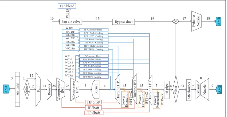
A brand new engine model was generated to provide high idelity and real-time gas turbine performance simulation. he model is representative of a three shat engine, which is the most complex engine architecture. Other existing jet engines architectures (single and 2 shat engines, mixed and unmixed lows) can be simulated by activating or deactivating components or entire shats, by deining pressure ratios and eiciencies equal to 1. Additionally, several bleed conigurations were modeled in order to give the user the ability to conigure the bleed port extraction position, the amount

of bleed extraction and the destination of the air being bled from the compressors: outboard bleed (for engine operability, aircrat air conditioning, pressurization, and anti-ice) as well as turbine cooling. In the case of the air being bled for turbine cooling purposes the user can select where exactly the cooling low will be inserted in the cycle: stators or rotors of the turbine stages. At last, the model can deal with power extraction from all the shats for aircrat systems. he schematics in Fig. 1 shows the engine model architecture with the airlow paths, power extractions, and power links (components mechanically linked through the shat) following the proposed nomenclature from SAE AS755. his diagram represents the most complex engine architure to be simulated.he model was built based on blocks with will calculate each engine module separately. he blocks developed for this model are:

• AMB (Standard Atmosphere): this block reads the Altitude, Flight velocity or Mach Number, Ambient temperature or deviation from standard day and air humidity and calculates the engine air inlet properties based on the U.S. Standard Atmosphere 1976, Antoine (1888), and Gordon (1982).

• Air Inlet: this block reads the ambient properties calculated by the Standard Atmosphere block, the input pressure recovery factor and calculates the air intake performance based on the MIL-E-5007D.

• Splitter: the mass low splitter block is used in several diferent places in the model, such as bypass and bleed

Figure 1. Three shaft direct drive engine model diagram.

AMB

A

ir I

n

let

Fan air valve

C

om

pr

es

sor

C

om

pr

es

sor

IPC HPC AMB

AMB

IP Shaft LP Shaft HP Shaft

HP Customer bleed

Fan bleed

P

o

w

er

E

xt

rac

tio

n

A

ft

erb

ur

n

er

E

xha

us

t

N

o

zzle

Je

t pip

e

T

urb

in

e HPT

T

urb

in

e IPT

T

urb

in

e LPT

B

ur

n

er

IP Customer bleed

B

o

os

ter 3 4 5

0 1

2

13

25 43 45

15 16

9 6 61 7

28 W B28

HPTP

w

rX

WB15

M

ix

er

Sp

li

ter

Fa

n

12

23

18

P

o

w

er

E

xt

rac

tio

n

IPTP

w

rX

LPTP

w

rX

Bypass duct 17

8

E

xha

us

t

N

o

zzle

WB3

HPT NGV Cooling HPT Blade Cooling IPT NGV Cooling IPT Blade Cooling LPT NGV Cooling LPT Blade Cooling HPT NGV Cooling HPT Blade Cooling IPT NGV Cooling IPT Blade Cooling LPT NGV Cooling LPT Blade Cooling

WC 28F WC 28E WC 28D WC 28C WC 28B WC 28A

WC3F WC3 E WC3 D WC3 C WC3A WC3 B

P

o

w

er

E

xt

rac

tio

(3)

348 Gazzetta Junior H, Bringhenti C, Barbosa JR, Tomita JT

extractions, and its basic function is to split the inlet low in two outlet lows with the same gas properties. • Compressor: this block reads the compressor characteristics,

such as pressure ratio and isentropic eiciency and calculates the gas outlet properties based on the inlet properties and gas compression as described in Saravanamuttoo et al. (2001). • Burner (Combustion Chamber): this block reads the

fuel characteristics, such as lower fuel heating value and hydrogen/carbon ratio, and combustion chamber characteristics, such as pressure ratio and exit temperature or fuel low and calculates the combustion gases properties based on inlet air properties as per Gordon(1982). • Turbine: the turbine block calculates the gas expansion based

on the turbine isentropic eiciency and inlet properties as described in Saravanamuttoo et al. (2001).

• Duct losses (Bypass duct and jet pipe): this block calculates the pressure loss through a duct given the pressure recovery factor.

• Mixer: this block calculates the resulting gas properties based on the 2 inlet gas lows. he calculation is based on the chemical composition, pressure, and temperature of each gas low.

• Exhaust Nozzle: this block calculates the exhaust gas properties and velocity, based on the nozzle inlet gas properties and nozzle coefficients and geometry (convergent or convergent-divergent), as well as gross thrust. Figure 2 shows the model simulation main process diagram. he lowchart represents all the engine blocks, libraries, input data and iterations necessary to simulate the engine performance. he main steps necessary to perform the simulation are:

• Design Point input read. his block reads all input data necessary to characterize the engine modules and calculate each block at design point.

• Calculate each engine module at component level in the sequence of the gas low in order to reach the Design Point performance at engine level.

• Read the components maps for of-design performance simulations.

• Scale the components maps based on each module performance previously calculated at Design Point.

• Output the simulation results and the components scaled maps for of-design simulation.

• Ater inishing the Design Point calculation read the of design inputs, such as operating condition and power setting.

• Set the iterative process starting point. In this model the starting point can be the set equal to the last successfully converged point or a pre-deined starting point calculated based on the light condition and power setting.

• Calculate the engine components performance and overall performance.

• Check if all the energy balances, mass low balance and power settings are respected. If so output the calculated engine performance else a new iteration shall be performed with the new operation condition calculated by Broyden or Newton-Raphson method for non-linear system of equation solving.

MODEL DESCRIPTION

he mathematical model described herein are simpliied for the sake of the reader clarity. More details can be obtained in the open literature as Mckinney (1967), Koenig and Fishback (1972), Fishback and Koenig (1972), Szuk (1974), Palmer and Yang (1974), Macmillan (1974), Sellers (1975), Wittenberg (1976), Flack (1990), Stamatis et al.(1990), Ismail and Bhinder (1991), Korakianitis and Wilson (1994), Baig and

Design point (DP)

DP input card

DP simulation

Off design point (ODP)

ODP input read

ODP simulation

Simulation converged First guess for iterative process

Components map reading

Components map scaling

Output of simulation results and scaled maps

Output of simulation results

Calculate new inputs using linear systems solvers

Yes

No

(4)

349

Real-Time Gas Turbine Model for Performance Simulations

Saravanamuttoo (1997), Bringhenti (1999), Saravanamuttoo

et al. (2001), Walsh and Fletcher (2004).

STANDARD ATMOSPHERE

h e Standard Atmosphere dei nition implemented in the model described in this paper is based on the U.S. Standard Atmosphere 1976. It splits the atmosphere in 5 dif erent levels up to 85 km grouping in the same level altitudes with similar characteristics of temperature and pressure variation as the altitude increases.

A summary of the atmosphere properties calculation for each atmosphere layer and the parameters to be used in static temperature and pressure calculation are described in Table 1.

where: g

’

₀ = 9.80665 m/s2_{is the geopotential gravity;}

M₀ = 28.96443 kg/mol is the air molecular weight; and

R* = 8,314.62 J/mol∙K is the universal gas constant.

HUMIDITY

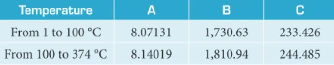
At all altitudes it is possible to set the humidity contained in the air. For this calculation the Antoine equation (Antoine 1888) determines the saturation vapor pressure for a given temperature for pure components. h e Antoine equation and constants for water are:

where: P_SATis the saturation pressure in mmHg; T_water is the water static temperature in °C; A, B, and C are constants that are specii c for each substance. h e constants for water are shown in Table 2.

Index (b) Layer Geopotential altitude Hb (km) Thermal gradient Lb (K/km) Reference temperature Tb (K) Reference pressure Pb (Pa)

0 Troposphere 0 –6.5 288.15 101,325.0000

1 Tropopause 11 0.0 216.65 22,631.9500

2

Stratosphere 20 +1.0 216.65 5,475.0960

3 32 +2.8 228.65 868.0107

4 Stratopause 47 0.0 270.65 110.9002

5

Mesosphere 51 –2.8 270.65 66.9383

6 71 –2.0 214.65 3.9563

Table 1. Standard atmosphere properties calculation summary table (U.S. Standard Atmosphere 1976).

Temperature A B C

From 1 to 100 °C 8.07131 1,730.63 233.426

From 100 to 374 °C 8.14019 1,810.94 244.485

Table 2. Constants for water saturation vapor pressure in Antoine equation.

INTAKE

h e engine air inlet simulation was implemented following the MIL-E-5007D, which describes the pressure recovery factors for subsonic, supersonic, and hypersonic l ows. Once the engine air inlet does no thermodynamic work and the l ow is considered adiabatic, the stagnation temperature through the duct remains constant. Air mass l ow and chemical composition also remain the same. h e stagnation pressure downstream the air inlet is calculated as follows:

Subsonic l ight (Mach < 1)

Supersonic l ight (1 ≤ Mach < 5)

(1) (3) (4) (5) (6) (2)



b



b

b L ALT H

T

T   





                                          



  



  



















                            







  





                   

 R Lb

M g b b b b b H ALT L T T P P * 0 ' 0                      



  



  



















                            







  





                                      b b T R H ALT M g b e P P * 0 ' 0     



  



  



















                            







  





                                      wa ter T C B A SAT P   10  



  



  



















                            







  





                                         IN OUT T

T RAMREC P

P  



  



  



















                            







  





                                          



1.35



) 1 ( 75 . 0

1  

 

RAMREC P MN

P IN OUT T T



















                            







  





                                          



  



             935 800 4 MN P RAMREC P IN OUT T T                             

Hypersonic l ight (Mach ≥ 5)

(5)

where Pt_IN is the inlet stagnation pressure in Pa; Pt_OUT is the outlet stagnation pressure in Pa; MN is the Mach Number;

RAMREC the engine air inlet pressure recovery (Pt_OUT/Pt_IN).

COMPRESSOR

he axial low compressor was implemented following the classic formulation described by Saravanamuttoo et al. (2001), Walsh and Fletcher (2004), and Kurzke (2007). The main equations in the compressor model are described as:

And the following equation is proposed for ER>1 considering the air limiting the combustion:

where: Y is the fuel hydrogen-carbon ratio; β is the water-air mass low ratio; α is (4+Y)/(4·ER).

The unburnt air is mixed to the combustion gases and the chemical composition of the gas leaving the burner is recalculated. Burner exit temperature can be either inputted or calculated based on the fuel low. In both cases, the following equation is used to calculate the temperature from fuel low or fuel low from temperature:







  





                                          



  



             IN OUT Pt Pt CPR                            







  





                                          



  



                                     1 1 1 1  

_c OUT_IN

IN OUT Pt Pt Tt Tt  







  





                                          



  



                                        IN OUT

Comp h h

w  

(8)

(9)

(13)

(14) (10)

he increase in the stagnation temperature due to work added to the airlow is calculated by:

and the thermodynamic speciic work is calculated by:

where: CPR is the compressor pressure ratio; Tt_IN is the inlet stagnation temperature in K; Tt_OUT is the outlet stagnation temperature in K; γ is the speciic heat ratio (Cp/Cv, being Cp and Cv the speciic heat at constant pressure and volume respectively); η_c is the compressor isentropic eiciency; w_Comp is the compressor speciic work in W/kg; h_IN is the inlet stagnation speciic enthalpy in J/kg; h_OUT is the outlet stagnation speciic enthalpy in J/kg.

COMBUSTION CHAMBER

he combustion chamber model calculates the amount of burnt fuel considering the amount of air and the equivalence ratio. Equivalence ratio is the ratio between the actual fuel air ratio and stoichiometric fuel air ratio, so equivalence ratio equal to 1 means stoichiometric burn, while lower and higher values mean lean and rich burns respectively. he chemical composition of the burnt gases is determined by the following equation, for equivalence ratio (ER) ≤ 1, as proposed by Gordon (1982):

(12)

(11)

where WF is the fuel low in kg/s; LFHV is the lower fuel heating value in J/kg; ṁ_IN is the mass low at burner inlet in kg/s; ṁ_OUT is the mass low at burnet outlet in kg/s; η_cc is the Ccombustion eiciency.

TURBINE

Turbine performance prediction is calculated as follows:

where η_t is the turbine isentropic eiciency.

he expansion through the turbine generates the necessary power to drive the compressor mechanically linked to the turbine by a shat. he turbine power can be calculated as follows:

(15)

where: ṁ is the gas mass low at turbine inlet in kg/s.

PROPELLING NOZZLE

In this model, 2 diferent nozzle geometries were implemented: convergent and convergent-divergent (con-di). For the con-di nozzle, 7 different flow configurations were implemented, as described by Devenport (2001) and Shapiro (1953). he









Y

Ar N O CH_Y           _ _             _ _                       ₂ 3.727587 ₂ 0.0447068 0.













                                          _                                        

 .00152



 



                                 



h



  

 

   

    

 

 

    

 x  

 

 

    

 x  



θ  π



θ 









          _ _             _ _                      













Ar N O CH_Y                                             _                                          ₂ 3.727587 ₂ 0.0447068 0



 



                                 



h 



  

 

   

     f x

 

 

    

  

 

 

    

  



θ  π



θ 









          _ _             _ _                      













O H Y Y CO Y CO Ar N O CHY                                             _                                          . 3 4 0015228 . 0 4 1 1 0015228 . 0 0447068 . 0 727587 . 3 2 2 2 2 2



 

h



                                 







  

 

   

    

 

 

    

  

 

 

    

  



θ  π



θ 









          _ _             _ _                      













                                          _                                         



 



                                 







 

 

   

    

 

 

    

  

 

 

    

  



θ  π



θ 









          _ _             _ _                      













N O                                             _                                          727587 . 3 ₂ 2 (



 



                                 







  

 

   

    

 

 

    

  

 

 

    

  



θ  π



θ 









          _ _             _ _                      













O Ar

Y Y

Y    

                                      _                                          0447068 . 0 4 2 4 1 1 1 4 2



 



                                 







  

 

   

    

 

 

    

  x

 

 

    

  x



θ  π



θ 









          _ _             _ _                      













O H CO Ar                                             _                                        

 0.0015228 2 2



 



                                 







  

 

   

    

 

 

    

  

 

 

    

  



θ  π



θ 









          _ _             _ _                      













                                          _                                         



 



cc IN IN OUT

OUT h m h

m LFHV WF                                  







  

 

   

    

 

 

    

  

 

 

    

  



θ  π



θ 









          _ _             _ _                      













                                          _                                         



 



                               1 1 1    IN OUT t IN OUT Pt Pt Tt Tt







  

 

   

    

 

 

    

  

 

 

    

  



θ  π



θ 









          _ _             _ _                      













                                          _                                         



 



                                 



hout hin



m

W  

 

   

    

 

 

    

  

 

 

    

  



θ  π



θ 









O H CO Ar           _ _             _ _                     

 0.0015228 2 2













                                          _                                         



 



                                 







  

 

   

    

 

 

    

  

 

 

    

  



θ  π



θ 









Y O H Y CO Ar N O CH_Y           _ _             _ _                       3 2 0015228 . 0 1 00 . 0 0447068 . 0 727587 . 3 2 2 2 2













                                          _                                          0015228



 



                                 



h



  

 

   

     x

 

 

    

  

 

 

    

  



θ  π



θ 









          _ _             _ _                       1













O                                             _                                         



 



                                 







  

 

   

    

 

 

    

  

 

 

    

  



θ  π



θ 









O N

CO Ar           _ _             _ _                       727587 . 3 0015228 . 0 2 2 2













O                                             _                                         



 



                                 







  

 

   

    

 

 

    

  

 

 

    

  



θ  π



θ 









Ar O

Y _ _ _ _

      _ _             _ _                       0447068 . 0 4 1 2 2













Ar                                             _                                          68



m

 



                                 





m 

 

 

   

     f

 

x

    

  

 

x

    

  

(6)

pressure distribution in the nozzle for each coniguration is shown in Fig. 3.

balance, and fuel low/Max cycle temperature constraint; variables: engine mass low, fan pressure ratio, IP compressor pressure ratio, HP compressor pressure ratio, HP turbine pressure ratio, IP turbine pressure ratio, LP turbine pressure ratio and fuel low).

he Broyden’s Method (Broyden 1965) was selected from trade study that was conducted to define which system of equations solver would give the shortest clock time to ind the solution.

he Broyden’s method is a generalization of the secant method to nonlinear systems. he secant method replaces the Newton’s method derivative by a inite diference:

GAS PROPERTIES

A good gas properties model is key for any thermodynamic cycle analysis. In order to keep the lexibility and accuracy of the engine performance simulations the gas properties model was developed with reined and detailed data from the Reference Fluid hermodynamic and Transport Properties (REFPROP; Lemmon et al. 2013). All the main gases present in the air and combustion gases composition (N₂, O₂, CO₂, Ar and H₂O) were modeled separately. he gas property is so calculated depending on its chemical composition and the partial contributions of each speciic gas enthalpy and molar mass. Enthalpy was modeled considering the efects of diferent temperatures and pressures.

OFF-DESIGN

The 3 major contributors who enabled the model to converge in few iterations and, therefore, short clock time were the powerful nonlinear system of equation solver, the maps interpolation method and the deinition of the starting point of the iterative process.

NON-LINEAR SYSTEM OF EQUATION SOLVER

For the 3 shat engine architectures the nonlinear system of equation is composed by 8 equations and 8 variables — equations: LP (low pressure) shat work balance, LP shat mass low balance, IP (intermediate pressure) shat work balance, IP shat mass low balance, HP (high pressure) shat work balance, HP shat mass low balance, engine core mass low Figure 3. Pressure distribution through the nozzle (Devenport 2001). (a) Not choked at throat; (b) Just choked at throat; (c) Shock in nozzle; (d) Shock at exit; (e) Overexpanded; (f) Design condition; (g) Underexpanded.

Throat Exit

Distance down the nozzle P / P_IN

1

0

(a) (b) (c) (d) (e) (f) (g)

(16)

(17)

(18)

where f is the function whose zeros are being searched; x is the free variable; k is the iteration number.

Broyden’s gave a system of equation generalization:

where J_F is the Jacobian calculated for the system of equations; F is a matrix with the solution of each equation calculated for x_k.

hus it is not necessary to calculate the Jacobian and all its derivatives of the Newton’s method in every iteration, therefore this method is time saving at a cost of slightly lower convergence rate.

MAPS INTERPOLATION METHOD

he developed computer program make use of maps for compressors and turbines for off-design calculation. The implemented method to find the operating condition and interpolate within the map values is based on linear interpolation. However, in order to improve the interpolation time, the search for the nearest points for interpolation was enhanced. Usually the map would be read from the irst line to the last looking for an interval that comprises the search point. It works ine if the interpolation point is close to the table head, usually close to the design point. However, the farthest the point is from the table head more data is necessary to be read and checked, which make the interpolation slow. In order to improve the searching for the nearest points it was implemented a procedure based on Point in Polygon (PIP) concept. he procedure consists in









  

    

  _ _ 

   

    

  _ _ 

  



   

 



 

 

 

 













   

  

  

    

  

      

   

    

 

   

  _

        

  

    

  

   

   

 















 





   

  

 

  

 

  

 

         

  









  

 

   

1 1

'

 

  

k k

k k k

x x

x f x f x f

 

 

    

  

 

 

    

  



θ  π



θ 









  

    

  _ _ 

   

    

  _ _ 

  



   

 



 

 

 

 













   

  

  

    

  

      

   

    

 

   

  _

        

  

    

  

   

   

 















 





   

  

 

  

 

  

 

         

  









  

 

   

 

  

 

1

    

1

'x_k x_kx_k_ f x_k f x_k_ f

 

 

    

  



θ  π



θ 









  

    

  _ _ 

   

    

  _ _ 

  



   

 



 

 

 

 













   

  

  

    

  

      

   

    



 _

  

  _

        

  

    

  

   

   

 















 





   

  

 

  

 

  

 

         

  









  

 

   

 

  

 

 

    

  

 

k k k1

    

 k  k1

F x x x f x f x

J



θ  π

(7)

divide the map in four quadrants and check if the interpolation point is within one of the quadrants. h e check is done by checking the sum of the angles between the interpolation point and the quadrant vertices. If the sum is 2π it means that it is in the quadrant and if it is 0, it is not. Once the quadrant that contains the interpolation point is found the same procedure is repeated reducing the quadrant size until the quadrant is formed only by the 4 nearest points, when it is ready for the interpolation. h e closest three points dei nes a plane that comprises the interpolation point and therefore the interpolation within the plane can be calculated. h e plane interpolation was implemented in order to avoid bilinear interpolation issues where the mass l ow is constant and the interpolation in mass l ow axis would lead to a division by 0.

Figure 4 shows a compressor map, as an example, and it is possible to observe how the map is divided into 4 quadrants successively until the quadrant is formed only by the 4 nearest points to the operating condition. Figure 5 shows how the angles between the operating point and the quadrant vertices shall be considered for PIP evaluation, whose possible values are described in Eqs. 19 and 20.

ITERATION STARTING POINT

Another extremely powerful feature of the model which improves both convergence success rate and time until the solution is the selection of the starting point close to the i nal solution. Obviously, the i nal solution is not known until the simulation is completed, but an approximation of the i nal solution can be estimated based on some engine parameters. In the model developed for this paper the engine parameters to start the iteration are set based on the l ight condition and the a power setting parameter. h e design point parameters are corrected to the of -design l ight condition and then corrected to the input power setting. h e power setting parameter dei nes the engine power such as fuel l ow, burner exit temperature and shaft speed. All of them can be set as input to the model.

MODEL VERIFICATION

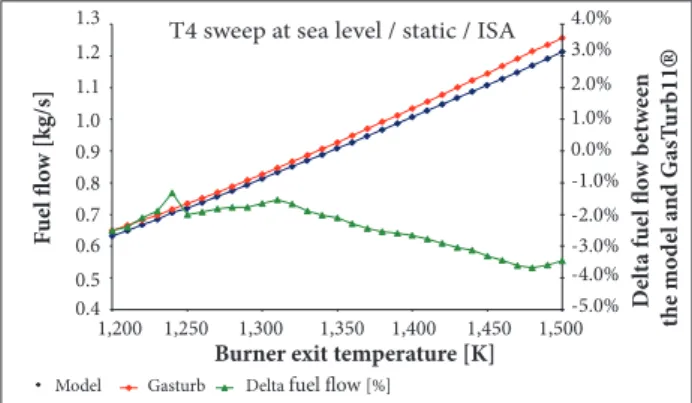
h e developed model was compared in terms of thrust and fuel l ow calculation with an existing commercial gas turbine performance model. h e model for reference was GasTurb11® (Kurzke 2007) which is very known, reliable and l exible to receive the same kind of inputs necessary to set the model developed for this paper. h e simulations, for all the 3 architectures, were based on a burner exit temperature sweep at ISA Sea Level Static condition and compared using the same compressors and turbine maps. Figures 6 to 11 show the comparison between the GasTurb11® and the developed model. h e divergences found in thrust and fuel l ow are due to dif erences in the combustion gas model. h e gas model in GasTurb11® does not consider pressure in the enthalpy calculation while the developed model does. Also, the combustion gases composition calculation may lead to dif erences in the cycle calculation mainly downstream to the burner. h e model could not be compared in terms of run time because no models were found in the literature with the ability to run in real time.

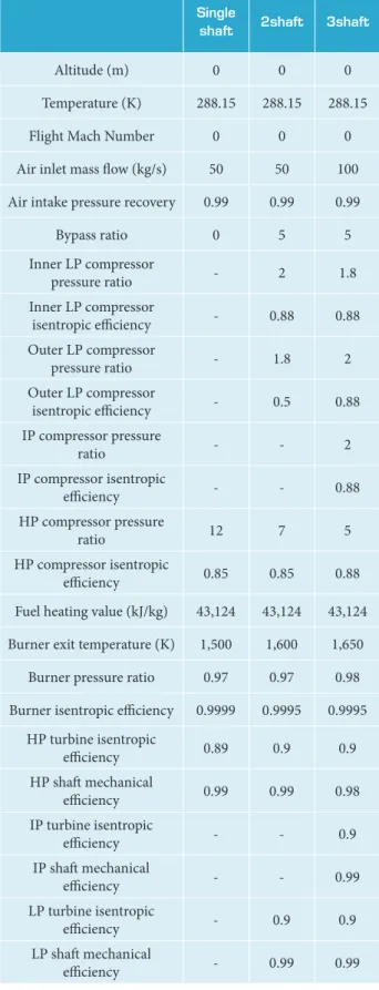
h ree dif erent engine architectures were simulated and compared in terms of thrust and fuel l ow with the engines modeled in GasTurb11® with same configuration. The architectures are the most utilized in the aeronautic industry: single, 2 and 3 shat s direct drive engines with unmixed l ows and convergent nozzles. h e Design Point of the models is shown in Table 3.

Figures 6 and 7 show the thrust and fuel l ow comparison with GasTurb11® for the turbojet architecture (one shat direct

P

r

ess

u

r

e r

a

ti

o

Co_rrected mass flow

Figure 4. Quadrant division example in a compressor map.

Figure 5. PIP graphic representation.

θ

If

Σ

θ_i= 2π then the point is within the polygon (19)

(8)

drive engine). Figures 8 and 9 show the same comparison for the 2 shat direct drive turbofan. Finally, Figs. 10 and 11 are the comparison between the models for 3 shaft direct drive turbofan engine.

In Figs. 6 and 7 the blue and red curves refer to the calculated parameters, thrust or fuel low, by this paper’s model and GasTurb11®, respectively, and the values are in the let vertical axis. he diference between the values calculated by the model described in this paper and Gasturb11® are shown by the green curve whose values are in the right

T4 sweep at sea level / static / ISA

10,000 15,000 20,000 25,000 30,000 35,000 40,000 45,000 50,000

1,200 1,250 1,300 1,350 1,400 1,450 1,500

Burner exit temperature [K]

Thr

us

t [N]

-2.0% -1.5% -1.0% -0.5% 0.0% 0.5% 1.0% 1.5% 2.0%

D

el

ta thr

us

t b

et

w

ee

n

the mo

d

el a

nd G

asT

urb11

®

Model Gasturb Delta thrust [%]

Thr

us

t [N]

D

el

ta thr

us

t b

et

w

ee

n

the mo

d

el a

nd G

asT

urb11

®

Burner exit temperature [K] Model Gasturb Delta thrust [%]

15,000 20,000 25,000 30,000 35,000 40,000 45,000

1,250 1,300 1,350 1,400 1,450 1,500 1,550 1,600 1,650-3.0% -2.0% -1.0% 0.0% 1.0% 2.0% 3.0%

B_{urner exit temperature [K]}

Thr

us

t [N]

D

el

ta thr

us

t b

et

w

e

en

the mo

d

el a

nd G

asT

urb11

®

Model Gasturb Delta thrust [%]

0 2,000 4,000 6,000 8,000 10,000 12,000 14,000 16,000 18,000 20,000

1,200 1,250 1,300 1,350 1,400 1,450 1,500 1,550 1,600 -2.5% -2.0% -1.5% -1.0% -0.5% 0.0% 0.5% 1.0% 1.5% 2.0% 2.5%

Model Gasturb Delta fuel flow [%]

0.4 0.5 0.6 0.7 0.8 0.9 1.0 1.1 1.2 1.3

1,200 1,250 1,300 1,350 1,400 1,450 1,500

F

u

e

l fl

o

w [kg/s]

-5.0% -4.0% -3.0% -2.0% -1.0% 0.0% 1.0% 2.0% 3.0% 4.0%

D

el

ta

f

u

el

fl

ow

b

etwe

en

the mo

d

el a

nd G

asT

urb11

®

D

el

ta

f

u

el

fl

ow

b

etwe

en

the mo

d

el a

nd G

asT

urb11

®

Model Gasturb Delta fuel flow [%]

0.0 0.1 0.2 0.3 0.4 0.5 0.6

1,250 1,300 1,350 1,400 1,450 1,500 1,550 1,600 1,650

F

u

el fl

o

w [kg/s]

-3.0% -2.0% -1.0% 0.0% 1.0% 2.0% 3.0%

D

el

ta

f

u

el

fl

ow

b

etwe

en

the mo

d

el a

nd G

asT

urb11

®

Model Gasturb Delta fuel flow[%]

0.05 0.07 0.09 0.11 0.13 0.15 0.17 0.19 0.21 0.23 0.25

1,200 1,250 1,300 1,350 1,400 1,450 1,500 1,550 1,600

F

u

el fl

o

w [kg/s]

-5.0% -4.0% -3.0% -2.0% -1.0% 0.0% 1.0% 2.0% 3.0% 4.0% 5.0%

Figure 6. Single shaft engine thrust comparison.

Figure 10. Three shaft simulated engine thrust comparison.

Figure 8. Two shaft simulated engine thrust comparison.

Figure 7. Single shaft simulated engine fuel low comparison.

Figure 11. Three shaft simulated engine fuel low comparison.

Figure 9. Two shaft simulated engine fuel low comparison.

vertical axis. Diferences are expected due to the gas properties model diferences and premises in the 2 diferent simulation tools.

(9)

Single

shaft 2shaft 3shaft

Altitude (m) 0 0 0

Temperature (K) 288.15 288.15 288.15

Flight Mach Number 0 0 0

Air inlet mass low (kg/s) 50 50 100

Air intake pressure recovery 0.99 0.99 0.99

Bypass ratio 0 5 5

Inner LP compressor

pressure ratio - 2 1.8

Inner LP compressor

isentropic eiciency - 0.88 0.88

Outer LP compressor

pressure ratio - 1.8 2

Outer LP compressor

isentropic eiciency - 0.5 0.88

IP compressor pressure

ratio - - 2

IP compressor isentropic

eiciency - - 0.88

HP compressor pressure

ratio 12 7 5

HP compressor isentropic

eiciency 0.85 0.85 0.88

Fuel heating value (kJ/kg) 43,124 43,124 43,124

Burner exit temperature (K) 1,500 1,600 1,650

Burner pressure ratio 0.97 0.97 0.98

Burner isentropic eiciency 0.9999 0.9995 0.9995

HP turbine isentropic

eiciency 0.89 0.9 0.9

HP shat mechanical

eiciency 0.99 0.99 0.98

IP turbine isentropic

eiciency - - 0.9

IP shat mechanical

eiciency - - 0.99

LP turbine isentropic

eiciency - 0.9 0.9

LP shat mechanical

eiciency - 0.99 0.99 Table 3. Simulated engines design point for output comparison with GasTurb11®.

assessment. Table 4 summarizes the chosen values used to simulate different engine operational conditions.

RESULTS

he run time distribution and the number of iterations until the convergence are shown in Figs. 12 and 13, respectively. he run times were achieved in a personal computer with Intel Core i7 920 at 2.67GHz and the solver convergence criteria was set to square root of the machine precision which was in the computer where the points were run, 10−8_{. he results are}

disposed in a histogram chart where it is shown the distribution of the number of converged points, in the ordinates, by the elapsed time until convergence (Fig. 12) or number or iterations until the convergence (Fig. 13), in abscissas. he points and the operating conditions evaluated are described in Table 4.

An additional run time reducing opportunity was assessed in order to improve the model run time: iteration stopping criteria relaxing. In order to provide accuracy in the calculations the stopping criteria was chosen to be the square root of the machine precision. Figure 14 shows that the model converges very quickly to the solution and spends a lot of iterations reining

Number of_iterations

N

um

b

er o

f p

o

in

ts

1 8 , 0 0 0 1 6 , 0 0 0 1 2 , 0 0 0 1 0 , 0 0 0 8 , 0 0 0 6 , 0 0 0 4 , 0 0 0 2 , 0 0 0 1 4 , 0 0 0

0

0 3 6 9 1 2 1 5 1 8 2 1 2 4 2 7 3 0 3 3 3 6 3 9 4 2 4 5 4 8 5 1 5 4 5 7 < 6 0

Figure 12. Run time histogram.

0 2,000 4,000 6,000 8,000 10,000 12,000 14,000 16,000 18,000

10 14 18 22 26 30 34 38 42 46 50 54 58 62 66 >70

N

um

b

er o

f p

o

in

ts

Run time [ms]

(10)

Similar result can be veriied in Fig. 16. he chart shows the beneit that the stopping criteria relaxing brought in terms of numbers of iterations. he peak and the average moved to the let, what means that more points converged at lower number of iterations.

Altitude Mach Number Delta standard day Burner exit temperature

Sea level - 15,000 m (steps of 500 m)

Static - 0.8 (steps of 0.05)

−30 °C +30 °C (steps of 5 °C)

1,800 K - 1,000 K (steps of 100 K)

Table 4. Simulation test matrix.

1 –0.02

0.00 0.02 0.04 0.06 0.08 0.10 0.12 0.14 0.16 0.18 0.20 0.22

2 3 4 5

Nozzle massflow balance

HPT massflow balance

LPT massflow balance

6 7 8 9

Interation n_umber

P

ar

am

et

er

v

a

lu

e

0 3 6 9 12 15 18 21 25, 000

20, 000

15, 000

10, 000

5, 000

0

24 27 30 33 36 39 42 45 48 51

10– 5

10– 8

54 57 60

Number o_{f iterations}

N

um

b

er o

f p

o

in

ts

10–5

10–8

0 2,000 4,000 6,000 8,000 10,000 12,000

10 12 14 16 18 20 22 24 26 28 30 32 34 36 38 40 42 44 46 48 50

Run time [ms]

N

um

b

er o

f p

o

in

ts

Figure 15. Stopping criteria relaxing beneit in run time.

Figure 14. Iteration steps until the solution.

Figure 16. Stopping criteria relaxing beneit in the number of iterations.

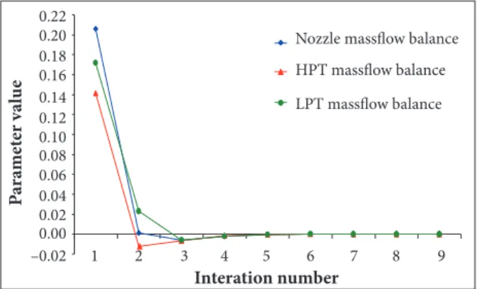
the solution to meet the very tight stopping criteria. he chart shows the evolution of 3 of the equations in the nonlinear system of equations for of design calculation. When the equation goes to 0 it means it converged. It can be seen that the parameters converge very quickly to the solution, approximately 4 iterations in the example, and require another 5 iteration to reine the inal solution to meet the excessively sharp stopping criteria.

he potential run time improvement due to the stopping criteria relaxation was assessed and the results are shown in Fig. 15. he chart shows the number of converged points in the ordinates and the run time in the abscissas. It can be seen that the peak and the average of the red columns, which represents the run time of the points with relaxed stopping criteria, are at lower run times when compared with the blue columns, which represents the points with original stopping criteria. It means that, by relaxing the stopping criteria, in general, the points converged faster, as expected.

CONCLUSIONS

A brand new engine performance prediction model was developed with the ability to run and reach the convergence in most of the times in less than 30ms, which is compatible with a high deinition video format, whose refresh rate is 30 frames per second. he features implemented in the model to improve the run time were very efective and ensure good model performance, within the target run time. Additionally, the model did not lose accuracy and flexibility with those features. In fact, by setting the starting point close to the inal solution, the convergence success rate was also improved. An additional feature which was also investigated, the relaxation in the iteration stopping criteria could improve even more the run time at a cost of some accuracy loss.

(11)

ACKNOWLEDGEMENTS

he inancial support from Empresa Brasileira de Aeronáutica (Embraer), Conselho Nacional de Desenvolvimento Cientíico e Tecnológico (CNPq), Centro de Pesquisa e Inovação Sueco-Brasileiro (CISB), and Svenska Aeroplan AB (SAAB) is acknowledged.

REFERENCES

Antoine C (1888) Tensions des vapeurs; nouvelle relation entre les tensions et les températures. Comptes Rendus des Séances de l’Académie des Sciences (in French). Paris.

Baig MF, Saravanamuttoo HIH (1997) Off-design performance prediction of single-spool turbojets using gasdynamics. J Propul Power 13(6):808-810. doi: 10.2514/2.5240

Bringhenti C (1999) Análise de desempenho de turbinas a gás em regime permanente (Master’s thesis). São José dos Campos: Instituto Tecnológico de Aeronáutica.

Bringhenti C (2003) Variable geometry gas turbine performance analysis (PhD thesis). São José dos Campos: Instituto Tecnológico de Aeronáutica. In Portuguese.

Broyden CG (1965) A class of methods for solving nonlinear simultaneous equations. Math Comp 19:577-593.

Devenport WJ (2001) Instructions; [accessed 2015 May 15]. http://www.engapplets.vt.edu/luids/CDnozzle/cdinfo.html

Fishback LH, Koenig RW (1972) GENENG II: A program for calculating design and off-design performance of two and three spool turbofans with as many as three nozzles. (NASA TN D-6553).Washington: NASA.

Flack RD (1990) Analysis and matching of gas turbine components. International Journal of Turbo and Jet Engines 7(3-4):217-226. doi: 10.1515/TJJ.1990.7.3-4.217

Gordon S (1982) Thermodynamic and transport combustion properties of hydrocarbons with air. Lewis Research Center Cleveland.

Grönstedt T (2000) Development of methods for analysis and optimization of complex jet engine systems (PhD thesis). Göteborg: Chalmers University of Technology.

Ismail IH, Bhinder FS (1991) Simulation of aircraift gas turbine engines. J Eng Gas Turbines Power 113(1):95-99. doi: 10.1115/1.2906536

Koenig RW, Fishback LH (1972) GENENG: A Program for calculating design and off-design performance for turbojet and turbofan engines. (NASA TN D-6552). Washington: NASA.

Korakianitis T, Wilson DG (1994) Models for predicting the performance of Brayton-cycle engines. J Eng Gas Turbines Power 116(2):381-388. doi: 10.1115/1.2906831

Kurzke J (2007) GasTurb11: design and off-design performance of gas turbines. Aachen: GasTurb GmbH.

Lemmon EW, Huber ML, McLinden MO (2013) NIST Standard Reference Database 23: Reference Fluid Thermodynamic and Transport Properties-REFPROP, Version 9.1. Gaithersburg: National Institute of Standards and Technology.

Macmillan WL (1974) Development of a modular type computer computer program for the calculation of gas turbine off-design performance. Cranield: Cranield Institute of Technology.

Mckinney JS (1967) Simulation of turbofan engine - SMOTE: Description of method and balancing technique. AD-825197/AFAPL-TR-67-125. Air Force Aero Propulsion Lab. pt.1-2.

Palmer JR, Yang CZ (1974) TURBOTRANS: A programming language for the performance simulation of arbitrary gas turbine engines with arbitrary control systems. ASME Paper 82-GT-200.

Saravanamuttoo HIH, Rogers GFC, Cohen H (2001) Gas turbine theory. 5th edition. New York: Prentice Hall.

Sellers JD (1975) DYNGEN: a program for calculating steady-state and transient performance of turbojet and turbofan engines. NASA TN D-7901. Washington: NASA.

Shapiro AH (1953) The dynamics and thermodynamics of compressible luid low. Vol. I-II. New York: The Ronald Press Company.

Silva FJS (2011) Gas turbines performance study under the inluence of variable geometry transients (PhD thesis). São José dos Campos: Instituto Tecnológico de Aeronáutica. In Portuguese.

Stamatis A, Mathioudakis K, Papailiou KD (1990) Adaptive simulation of gas turbine performance. J Eng Gas Turbines Power 112(2):168-175. doi: 10.1115/1.2906157

Szuk JR (1974) HYDES: a generalized hybrid computer program for studying turbojet or turbofan engine dynamics. NASA TM X-3014. Washington: NASA.

Walsh PP, Fletcher P (2004) Gas turbine performance. 2nd edition. Oxford: Blackwell Science.

Wittenberg H (1976) Prediction of off-design performance of turbojet and turbofan engines. CP-242-76, AGARD.

AUTHOR’S CONTRIBUTION