RBRH, Porto Alegre, v. 21, n. 4, p. 855-870, out./dez. 2016 Scientiic/Technical Article
http://dx.doi.org/10.1590/2318-0331.011616086
Real-time updating of HEC-RAS model for streamlow forecasting using an
optimization algorithm
Atualização em tempo real do modelo HEC-RAS para previsão de vazões utilizando um algoritmo de otimização
Vinícius Alencar Siqueira1, Mino Viana Sorribas1, Juan Martin Bravo1, Walter Collischonn1,
Auder Machado Vieira Lisboa2 and Giovanni Gomes Villa Trinidad2
1Universidade Federal do Rio Grande do Sul, Porto Alegre, RS, Brazil 2Itaipu Binacional, Foz do Iguaçu, PR, Brazil
E-mails: [email protected] (VAS), [email protected] (MVS), [email protected] (JMB), [email protected] (WC), [email protected] (AMVL), [email protected] (GGVL)
Received: June 21, 2016 - Revised: August 16, 2016 - Accepted: August 19, 2016
ABSTRACT
Real-time updating of channel low routing models is essential for error reduction in hydrological forecasting. Recent updating techniques found in scientiic literature, although very promising, are complex and often applied in models that demand much time and expert knowledge for their development, posing challenges for using in an operational context. Since powerful and well-known computational
tools are currently available, which provide easy-to-use and less time-consuming platforms for preparation of hydrodynamic models, it becomes interesting to develop updating techniques adaptable to such tools, taking full advantage of previously calibrated models as
well as the experience of the users. In this work, we present a real-time updating procedure for streamlow forecasting in HEC-RAS model, using the Shufled Complex Evolution - University of Arizona (SCE-UA) optimization algorithm. The procedure consists in a simultaneous correction of boundary conditions and model parameters through: (i) generation of a lateral inlow, based on Soil
Conservation Service (SCS) dimensionless unit hydrograph and; (ii) estimation of Manning roughness in the river channel. The algorithm works in an optimization window in order to minimize an objective function, given by the weighted sum of squared errors between
simulated and observed lows where differences in later intervals (start of forecast) are more penalized. As a case study, the procedure was applied in a river reach between Salto Caxias dam and Hotel Cataratas stream gauge, located in the Lower Iguazu Basin. Results showed that, with a small population of candidate solutions in the optimization algorithm, it is possible to eficiently improve the model performance for streamlow forecasting and reduce negative effects caused by lag errors in simulation. An advantage of the developed procedure is the reduction of both excessive handling of external iles and manual adjustments of HEC-RAS model, which
is important when operational decisions must be taken in relatively short times.
Keywords: River low forecasting; HEC-RAS; Real-time updating; SCE-UA.
RESUMO
A atualização em tempo real de modelos de propagação do escoamento em rios é essencial para a redução de erros na previsão
INTRODUCTION
One of the greatest challenges of reservoir operation relies in our ability to anticipate future conditions of a river system. This can be achieved through a hydrological forecast, in
which variables such as streamlow and river stage are predicted with suficient lead time to support decision-making procedures. Especially during occurrence of loods, decisions about gate opening and closing are extremely important in order to prevent
loss of human life and damage of infrastructure, whilst in many cases must be taken in short time intervals (e.g. few hours) under stress conditions.
Hydrological forecasting can be performed through a myriad of
mathematical models, ranging from statistical upstream-downstream relationships to physically-based routing models described by full
1D Saint-Venant equations. Historically, the latter approach has
received little attention due to its high computational burden, detailed
topography requirements and greater complexity regarding statistical
methods. These limitations have been overcome with technological advances of the last decade (PAIVA; COLLISCHONN; TUCCI, 2011), giving rise to software packages that provide easy-to-use and low time-consuming platforms for preparation of hydrodynamic
models. For instance, the HEC-RAS model, which is widely used
in traditional engineering problems (e.g. CESTARI JUNIOR;
SOBRINHO; OLIVEIRA, 2015; RIBEIRO NETO et al., 2015;
MONTE et al., 2016) and scientiic studies covering large complex
river systems (e.g PAZ et al., 2010; BRAVO et al., 2012), has been
successfully applied in institutions related to operational streamlow
forecast (e.g. HICKS; PEACOCK, 2005; MOREDA et al., 2009;
ADAMS; CHEN; HEIN, 2011; MASHRIQUI et al., 2014). In
the Brazilian context, a partnership signed in 2013 between the Brazilian National Water Agency (ANA) and the US Army Corps of Engineers (USACE) is currently motivating the use of
HEC-RAS and other modelling tools for water resource management,
including lood control and real-time reservoir operation. However, when hydrological forecasting is performed using
a physically-based routing model, differences between calculated and observed values are routinely noticed even for intervals prior to the start of forecast. These differences usually emerge from errors
in the input data and simpliications/parameterizations adopted
in related physical processes (MASKEY et al., 2004; CLOKE;
PAPPENBERGER, 2009; ZAPPA et al., 2011; MELLER et al., 2012), which can be reduced with a common procedure called
model updating or data assimilation. Potential beneits and opportunities of data assimilation have been extensively discussed
since the 80s (e.g. O’CONNEL; CLARKE, 1981; LIU et al.,
2012), and currently it is treated as an optimal combination of model output and independent observations to quantify and minimize uncertainties in model predictions (LIU et al., 2012). In hydrodynamic models, where physics are relatively well represented, major uncertainties can arise from instability of the numerical scheme, boundary conditions derived from rating-curves,
coeficients (e.g. roughness, hydraulic structures) and geometry of
the cross sections (PAPPENBERGER et al., 2005; RICCI et al., 2011; DOMENEGHETTI; CASTELLARIN; BRATH, 2012;
HABERT et al., 2016).
In general, model updating is conducted through four different approaches. These include corrections of model input, output, parameters or state variables (REFSGAARD, 1997; NEAL et al., 2007; MELLER et al., 2012), and it can be done using stochastic methods (e.g. BABOVIC et al., 2001; ROMANOWICZ et al., 2008), deterministic empirical techniques (e.g. PAZ et al., 2007),
or more sophisticated methods such as particle iltering and variations of Kalman Filter (e.g. MADSEN; STOKNER, 2005;
NEAL et al., 2007; RICCI et al., 2011; HABERT et al., 2016). In a brief literature review, Hsu et al. (2003, 2006) updated, respectively,
the simulated stage and the Manning coeficient of a hydrodynamic
model, through a minimization of a least-square error function. Ricci et al. (2011) used the Ensemble Kalman Filter (KF) to update
both upstream lows and model hydraulic state variables during lood events, occurring in two French catchments. Wu et al. (2013) developed a real-time forecasting model for Yangtze river operation of the Three Gorges reservoir, combining the Ensemble KF to a
hydrodynamic model. In a recent study, Habert et al. (2016) applied
an Extended KF to update boundary conditions (i.e. upstream and lateral inlows) and friction coeficients using, respectively,
observed discharge and observed water level.
Although iltering techniques are the state-of-the-art in scientiic research and, indeed, very promising for model updating in streamlow forecast, some shortcomings still remain when these
methods are applied for operational purposes. In general, these
techniques are very complex and require a good understanding
of total uncertainty to provide useful results, which is not a straightforward task in practical situations (ROMANOWICZ et al., 2008; LIU et al., 2012). In addition, models used for testing such
techniques are often very speciic and demand much time and expert knowledge for their development, posing challenges for
operational institutions since robust and easily handled models are rather preferable.
Therefore, the development of adaptable techniques to widely known computational platforms becomes interesting, and a O algoritmo opera em uma janela de otimização com a minimização de uma função-objetivo, que considera a soma ponderada dos erros
quadráticos das vazões dando maior peso aos erros nos últimos intervalos com dados observados (início da previsão). Como estudo de caso, a metodologia foi aplicada em um trecho localizado na bacia do rio Iguaçu, entre a UHE Salto Caxias e o posto luviométrico de Hotel Cataratas. Os resultados mostraram que, com um conjunto relativamente pequeno de soluções candidatas no algoritmo de otimização, é possível melhorar, de forma eiciente, o desempenho do modelo na previsão de vazões e reduzir efeitos negativos
causados por erros de fase nos hidrogramas calculados. Uma vantagem da metodologia desenvolvida é que ela permite reduzir tanto
a necessidade de manipulações excessivas de arquivos como de ajustes manuais do modelo HEC-RAS, o que é importante quando decisões operacionais devem ser tomadas em tempo relativamente curto.
possible approach consists in the use of optimization algorithms.
Although rarely explored for data assimilation in lood forecasting
models (e.g. MEDIERO; GARROTE; CHAVEZ-JIMENEZ, 2012), some recent studies have shown the potential of these
algorithms when combined to models such as HEC-RAS and
other similar software packages. In most of the cases, global search heuristic algorithms (e.g evolutionary algorithms) are used to solve multi-purpose reservoir problems (e.g. NGO et al., 2007; MALEKMOHAMMADI et al., 2010; CHE; MAYS, 2015;
BASHIRI-ATRABI et al., 2015) as well as optimal estimation
of the Manning coeficient (e.g. AYVAZ, 2013; YANG et al., 2014). Inspired by the aforementioned studies, the objective of this work is to present a simple method of real-time updating of
HEC-RAS model for streamlow forecast using a global search
optimization algorithm.
This paper is organized as follows. Firstly, the hydraulic
model (HEC-RAS) and the SCE-UA algorithm are briely described. Next, estimation of a lateral inlow and optimization details are presented, as well as the procedure for coupling HEC-RAS with
SCE-UA. Finally, the updating method is tested in a tributary of Parana river as a study case.
METHODS
Herein, the updating of HEC-RAS model is given as a
deterministic data assimilation, in which internal boundary conditions and model parameters are estimated based on downstream real
time observed discharge. Considering a situation where the low of tributaries for a speciic river reach is unknown, model calculations
are corrected by applying the global search algorithm to estimate the
“optimal” lateral inlow, so that model underestimation in output lows can be addressed. Furthermore, the Manning coeficient is
simultaneously adjusted by the optimization algorithm, which is
justiied by uncertainty in upstream lows, errors in geometry of
cross sections (PAPPENBERGER et al., 2005; DOMENEGHETTI;
CASTELLARIN; BRATH, 2012) and variations of channel
roughness for different low conditions (HSU et al., 2006).
HEC-RAS model
HEC-RAS is a widely used hydraulic model for river low simulation, which is developed by the Hydrological Engineering
Center/U.S. Army Corps of Engineers (HEC; USACE, 2010).
In its current version, the HEC-RAS allows the numerical solution of the full 1D Saint-Venant equations and determination of low
characteristics under steady or unsteady conditions, providing a friendly graphical user interface for data handling and visualization of model results.
The Saint-Venant equations are represented through conservation of mass and momentum. In the former case, conservation of mass (Equation 1) for a volume control states that the rate of change in storage must be equal to the net rate of
low into the volume, given as (HEC; USACE, 2010):
l
A Q
q
t x
∂ +∂ =
∂ ∂ (1)
Where: “A” represents the cross section wetted area in the volume control; Q is the streamlow and; ql is the lateral inlow per unit length.
Conversely, the net rate of momentum entering the volume
plus the sum of external forces acting on the volume control are
equal to the rate of accumulation of momentum (Equation 2). This is also known as the dynamic wave equation:
( )
. . f
Q Qu g A z S 0
t x x
∂ +∂ + ∂ + =
∂ ∂ ∂ (2)
Where: u is the mean velocity of low along the ‘x’ direction; z is the water elevation (relative to a datum); Sf is the friction slope, which is commonly written as the Manning equation for uniform,
steady low (Equation 3):
4 2 3
²
f
H
n Q Q
S
R A
= (3)
Where: RH is the hydraulic radius and; n is the Manning coeficient.
SCE-UA algorithm
The SCE-UA algorithm (Shufled Complex Evolution –
University of Arizona) (DUAN et al., 1992) combines the search
strategies of the Simplex method (NELDER; MEAD, 1965) with
concepts of random search, competitive evolution and complex shufling. This algorithm has shown suitable results regarding
parameter estimation, especially for calibration of hydrological models (e.g. DUAN et al., 1992; BREDA; GONÇALVES; SILVEIRA, 2011) and reservoir optimization (e.g. NGO et al., 2007; BRAVO et al., 2008).
Briely summarized, the SCE-UA performs with a population
(s) of points - or solutions - that evolves towards the global optimum of a mono-objective function, which is continuously evaluated through successive iterations. Solutions are ranked according to their objective function and are partitioned into
complexes, giving rise to offspring through a sequence of steps based on Simplex algorithm. Inside a complex, a given solution (parent) is replaced by an offspring if the latter is better itted
than the former one, and after a number of evolutionary steps,
the complexes are shufled. This procedure is repeated until the convergence criteria are satisied and the objective function is minimized. Parameters of the algorithm that must be deined are the number of complexes and number of individuals in each complex. Usually, values are selected so that c ≥ 1 and p ≥ 2n + 1, where c represents the number of complexes, p the number of
points in each complex and n the number of decision variables in the optimization problem. The population size is equal to c times p. Further details about the algorithm can be found in Duan et al. (1992).
Estimation of a lateral inlfow
For simplicity and due to a small number of necessary
parameters, the standard SCS dimensionless unit hydrograph (DUH)
lateral inlow. However, some changes in the gamma equation of
the original method were done as following (Equation 4):
( )
i t NTw tdi
λ = − −
when λ≥0
( ) exp( ). .exp . ,
m
i i
i i
p p
Q t m m Qp
T T
λ λ
= −
(4)
when λ<0
( ) i
Q t =0
Where: Qi(t) is the streamlow for time interval t and i hydrograph (m3s-1); NTw is the number of time intervals in HEC-RAS model
warmup; Tp is the peak time of the hydrographs (h); Qpi is the
peak low of i hydrograph (m3s-1); m is the gamma equation shape
factor; tdi is the displacement in peak time, for the i hydrograph (h).
The lateral inlow (Equation 5) is computed by the sum of the individual (synthetic) hydrographs obtained with the modiied gamma equation and by adding a baselow:
[ ]
1
( ) Nhidro ( )
lat i base
i
Q t Q t Q
=
= ∑ + (5)
Where: Qlat(t) is the lateral low for t time interval (m3s-1); Nhidro is
the total number of synthetic SCS hydrographs; Qbase is a variable
baselow.
Therefore, one or more synthetic hydrographs can be used
to generate the lateral inlow, considering the optimization of decision variables Qbase, Qpi and tdi, (i = 1, ..., Nhidro). Parameters Tp and m represent, respectively, the rise time of a typical basin
hydrograph and a shape factor related to the DUH peak rate factor
(m = 3.7 for standard DUH), which were held ixed during the optimization procedure. The total number of hydrograph intervals corresponds to the whole simulation period, from the warmup of
HEC-RAS model up to the end of forecast range.
Regarding the decision variables, parameter Qp is the
magnitude of the lateral inlow, in which the limits of the search space can be deined from a comparison between downstream
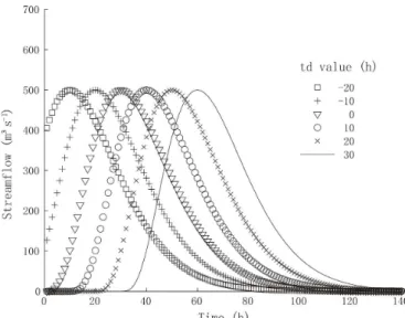
simulated and observed hydrographs. In addition, td represents the displacement in peak position in relation to the time of rise (Tp), changing the instant of its occurrence while preserving the original shape of the hydrograph. For instance, considering a Tp equivalent to 30 hours, a td value of 20 means that the peak instant occurs in t = 50 hours, while a td value of -10 indicates that the peak occurrence is at t = 20 hours. In order to illustrate this approach, Figure 1 shows a set of hydrographs generated with a Qp = 500 m3s-1 and a Tp = 30 hours, but with different values of
td, representing the displacement in peak position.
The lateral inlow is inserted in HEC-RAS model in a
lumped way into an intermediate cross section, which can be in
a speciic tributary or after the conluence of the most important rivers along the simulated reach. Nevertheless, this method can
be easily adapted in order to consider a uniformly distributed
lateral inlow.
Deining a mono-objective optimization function for model updating
An optimization procedure is then performed in order to solve the updating problem, i.e., the estimation of decision
variables corresponding to both lateral inlow parameters and Manning coeficient. For this, the SCE-UA algorithm runs in a
time window similar to that one used by Ricci et al. (2011), deined here as the “optimization window”. This window starts after the conclusion of warmup period and remains until the last interval with available real time observed data, which coincides with the start of forecast. The objective function (Equation 6) is computed as the sum of squared errors between simulated and observed values over the optimization window, but weighted according to the analyzed time interval:
( )2
. ( )
NTw NTotim
t t
t NTw
FO + Qcalc Qobs w t
=
= ∑ − (6)
subject to:
(i) tdmin≤td tdi≤ max
(ii) Qpmin≤Qp Qpi≤ max
(iii) Manningmin≤Manningi≤Manningmax
(iv) Qbasemin≤Qbase Qbasei≤ max
Where: FO is the objective function to be minimized; Qcalct is
the simulated low in time interval t, computed for the cross section where observed data is available; Qobst is the observed data in time interval t; w(t) is a weight function that depends on the analyzed time interval; NTw is the number of time intervals for model warmup and; NTotim is the number of time intervals in the optimization window.
The w(t) function (Equation 7) was introduced so that the weight of errors are increased for latter time intervals along the
optimization window. This is justiied by the fact that a better
agreement of calculated and observed values right before the start
of a forecast is desirable, since errors in the predicted lows can
be reduced especially for earlier forecast lead times. Thus, w(t) was undertaken in terms of a cubic function, described as following:
3
( ) t NTw
w t
NTotim
−
= (7)
Where: t is the simulation time interval. The weighted function w(t) is maximized (equal to unity) in the last time interval of the optimization window.
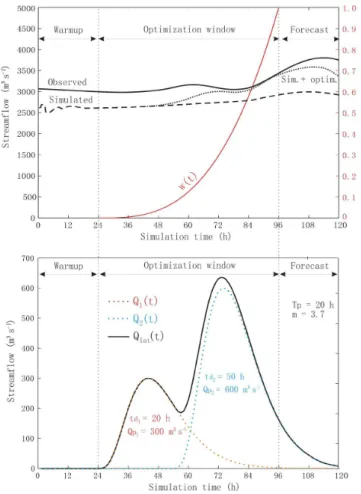
Figure 2 shows a graphical example of the model updating considering a warmup period of 24 hours, an optimization
window of 72 hours and a lateral inlow composed by two synthetic hydrographs. However, it is important to mention that a large optimization window can cause excessive weights for a
large number of time intervals, and in this case a less agreement between simulated and observed discharge is likely to occur right before the start of forecast. Conversely, a small time window can
be insuficient to properly optimize the Manning coeficient or to route the lateral inlow hydrograph to the downstream river
gauge, for which the objective function is calculated.
Coupling SCE-UA + HEC-RAS model for real time streamlow forecast
In order to perform a simultaneous run of SCE-UA
optimization and HEC-RAS model, a coupling algorithm was developed in VB.NET language using the HECRASController module (GOODELL, 2014; LEON; GOODELL, 2016). This controller provides a set of computational subroutines that
allows the full automation of HEC-RAS model, including data
input, simulation and results acquisition. Changes in Manning
coeficient can be done directly in HECRASController module, just indicating the cross sections where this parameter must be
set. On the other hand, deinition of both simulation period and inlow data for each model run require the external manipulation of speciic iles associated to HEC-RAS project (.prj), which are (HEC; USACE, 2010):
• Plan ile: refers to the ile with “.p” extension, where dates
of start and end of simulation are set;
• Unsteady low data ile: refers to the ile with “.u” extension,
where initial conditions, boundary conditions and lateral
inlow data are set.
Moreover, parameters of the coupling algorithm that
are needed to handle these iles are deined here as simulation
parameters:
• Nhidro: number of synthetic hydrographs;
• NT_warmup: number of time intervals for model warmup;
• NT_otim: number of time intervals for the optimization window;
• NT_prev: number of time intervals for the forecast range;
• NT_sim: number of time intervals for the simulation period, equal to: NT_warmup + NT_otim + NT_prev.
The simulation period in HEC-RAS model must be conigured to have the same number of time intervals as NT_sim. It is important to emphasize that the synthetic hydrographs must comprise all the simulation period, so that the model has enough
data for streamlow computations along the forecast range.
Likewise, additional data must be set in the upstream boundary
condition to represent the low in forecast intervals, which can
be a constant value such as the persistence of the last observed
discharge, for example.
Regarding the SCE-UA algorithm, the initial population of candidate solutions (s) are randomly generated within the limits
of the search space, considering the parameters Qbase, Qp, td and
Manning coeficient. Each of the individuals in s population is
composed by a single value of Manning coeficient and a single value of Qbase, as well as Nhidro parameters of both Qpi and tdi.
After applying the standard DUH gamma equation, the resulting
synthetic hydrographs must have NT_sim time intervals and be
further summed to compose the lateral inlow, which is inserted in a lumped way in a speciic cross section (set in the Unsteady low ile). Manning coeficient is uniformly set in channel of all cross sections and the HEC-RAS model is run, allowing to obtain the low at the point of interest and the calculation of the
objective function. After determining the FO for each individual in the population, the algorithm starts the evolutionary process Figure 2. Example of the model updating considering an
optimization window of 72 hours (24-96 h). The above illustration
shows the simulation being inluenced by the weighted function
w(t), so that simulated lows get closer to the observed values especially for later optimization intervals (Sim. + optim.). The
illustration below shows the lateral inlow (Qlat) generated by the
(SCE-UA Evolution) and the hydraulic model is internally called whenever the FO needs to be evaluated.
Only the maximum number of SCE-UA generations is
used as the convergence criterion. After ending, the algorithm
selects the best candidate solution among the inal population of individuals to provide the lateral inlow parameters and the estimated Manning coeficient. Figure 3 presents a simpliied low chart of SCE-UA and HEC-RAS model coupling with the main
steps of the real time updating procedure.
TESTING THE UPDATING PROCEDURE
Study case: Lower Iguazu basin
The Iguazu river basin has a total area of 70000 km2 and
lies between the states of Parana and Santa Catarina, in southern Brazil. Rainfall is relatively well distributed throughout the year and its annual average has an increasing gradient along east-west direction, from 1400 mm in the headwaters to about 2000 mm
near the conluence with Paraná River (DEMARIA et al., 2014).
A cascade of hydropower plants is found downstream of Uniao da Vitoria city in the Upper Iguazu, and some of the
reservoirs are used for both energy production and lood control
purposes. Due to the geomorphological and climatic characteristics of the basin, tributaries may have rapid rise of the hydrograph with very high peaks (REYNAUD; MINE; KAVISKI, 2014),
posing challenges for streamlow forecasting which is sometimes
performed by coupling stochastic or hydrological models to numerical weather prediction (e.g. GUILHON; ROCHA; MOREIRA, 2007; CASTANHARO et al., 2007; FIGUEIREDO et al., 2007; ARAUJO et al., 2014).
In the lower part of the basin, the maximum hourly and daily low variations are constrained in a streamgauge called R-11, located a few hundred meters downstream of the conluence with
Parana river. These constraints were imposed by international agreements such as the Tripartite signed by Brazil, Argentina and Paraguay in October 1979, ensuring safety of the population in
areas subject to looding (FERREIRA; SOARES FILHO, 2012). To meet the constraints, the operation of Itaipu reservoir in Parana
River depends on the predicted lows of Acaray and Monday rivers on the right bank and especially the lows of Iguazu river on the left bank, since high peak lows may occur in the latter during loods.
A HEC-RAS model is already set for this river system in
order to support the operation of Itaipu reservoir. For the lower
Iguazu basin, model is extended approximately 220 km up to Salto Caxias reservoir encompassing a drainage area of 10380 km2
(Figure 4), which is characterized by a sparse real time monitoring
network. Since the tributaries along this reach are not considered
in the hydraulic model, lows calculated in the last gauge station (Hotel Cataratas) are underestimated (Figure 5), which undermines
the effectiveness of streamlow forecasting in R-11. Therefore,
the local forecaster must estimate and manually enter a lateral
inlow in HEC-RAS model to address this problem, turning into
a time-consuming trial and error process.
Thus, the updating procedure was applied for the reach
between Salto Caxias reservoir and Hotel Cataratas river gauge, which was extracted from the Itaipu HEC-RAS model. Detailed
channel bathymetry is available for each 5 km on average, while
3 arc-sec SRTM data (FARR et al., 2007) is used for a roughly
representation of loodplain geometry. Upstream boundary condition is deined by hourly outlows of Salto Caxias reservoir,
whereas the downstream condition is given by friction slope for
normal depth. Right after Hotel Cataratas gauge, the Iguazu
Falls are represented by an inline weir with equivalent width to
the Iguazu River at this point. Also, observed data from Hotel
Cataratas gauge was available in hourly time interval comprising
the years of 2013 and 2014.
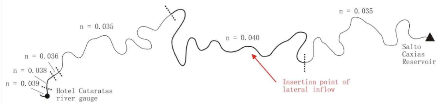
Figure 6 shows the original coniguration of HEC-RAS
model in terms of Manning coeficient, which was calibrated based
on observed river stage. For the updating procedure, the lateral
inlow was inserted approximately 110 km upstream of Hotel
Cataratas gauge, taking into account the main tributaries of this reach including Cotegipe, Sao Salvador, Capanema, Gonçalves Dias and Santo Antonio rivers.
The 5.0 Beta version of the HEC-RAS model was run
using an Intel Core i5 3.46 GHz (64 bits) processor with 8 Gb of RAM. Simulation parameters for testing the methodology were chosen as following:
- Nhidro = 2 synthetic hydrographs for generation of lateral
inlow. The gamma shape factor (m) adopted was the same
as the standard SCS DUH, equivalent to 3.7 (NRCS; USDA,
2007). Rise time (Tp) was ixed in 20 hours according to observed data from Capanema river.
- NT_warmup = 72 hours. In a test model run, this warmup period was long enough to address instabilities in the initial condition.
- NT_otim = 72 hours. As shown in Figure 2, a time window with NT_otim = 72 indicates that lows in the last 14 optimization intervals have a weight of above 50% in the objective function. These 14 time intervals are
suficient to characterize both rising and recession limb of the hydrograph in Hotel Cataratas, according to daily operation cycle of Salto Caxias reservoir.
- NT_prev = 24 hours. This forecast range was chosen
because travel time between Salto Caxias and Hotel Cataratas
is around 20 hours, considering normal conditions of reservoir operation.
For a Nhidro = 2, six decision variables (n = 6) are deined for SCE-UA: td1, td2, Qp1, Qp2, Qbase and Manning. The minimum
and maximum limits used for each one of these variables are
shown in Table 1. In respect to the maximum limit of td, a value equivalent to NT_otim-Tp was used in order to avoid the occurrence of peaks after the end of optimization window.
RESULTS AND DISCUSSION
Convergence of SCE-UA and real time applicability of the coupling algorithm
Firstly, the coupling algorithm was evaluated in terms of convergence of SCE-UA in order to verify its computational performance. Three different setups of the SCE-UA parameters (Table 2) were deined within the recommended range by Duan et al. (1992), from a minimum number of individuals in
each complex (p=n+1) to a number of p=2n+1. Other parameters
such as the number of points in each subcomplex (q), number
of consecutive offspring generated by subcomplex (α) and the number of evolutions in each complex (β) were held the same as
in Duan et al. (1992) and Santos, Suzuki and Watanabe (2003), equivalent to n + 1, 1 and 2n + 1, respectively.
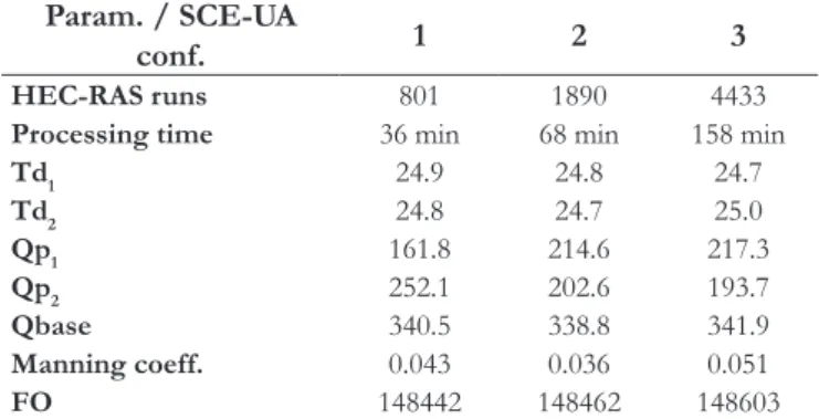
A time window with NT_sim intervals was randomly chosen within the available data period. Table 3 shows the total number of simulations and the estimated variables after the end of optimization procedure. For each run, the average time necessary
for the HEC-RAS evaluation was little more than 2 seconds. Except for the Manning coeficient, results were similar among tested conigurations, since the objective function was minimized
in all cases with a small difference between the estimated variables.
Regarding the computational eficiency, processing time was directly related to the number of HEC-RAS simulations, which in turn is linked mainly to the number of complexes in SCE-UA algorithm. For a value of β = 2n + 1, i.e, 13 evolution steps for
each complex in each generation, only the setup 1 completed the
optimization procedure in less than 1 hour.
Figure 7 shows the best solution for each setup over SCE-UA generations, and the square root of the FO was adopted for viewing purposes. For a larger number of individuals in the population Figure 5. Differences between observed and simulated lows
(HEC-RAS) in Hotel Cataratas river gauge.
Figure 6. Manning coeffcients (channel) retrieved from the original HEC-RAS model and insertion point of the estimated lateral
(e.g setup 3), the objective function in the initial generation tends
to be smaller, which is expected due to a better coverage of the
search space. Conversely, convergence becomes slower as much
as the size of the population is increased. For setup 3, almost 30 generations were needed in order to minimize the objective
function, while for the other cases, the convergence of SCE-UA
occurred with approximately 15 generations.
Whereas decisions about gate opening and closing must
occur in short time intervals, a less processing time coniguration
of the coupling algorithm becomes essential. Therefore, even if a
smaller number of complexes may result in a lack of information
in the search space and, consequently, an easier convergence to a local optimum (BREDA et al., 2011), a set of SCE-UA parameters
similar to setup 1 may be preferable for an operational context. In this way, real time updating of HEC-RAS model can be relatively eficient.
Statistical assessment of the updating method
A second test was carried out to assess the performance of the updating method in a long period, encompassing both low
and high low values. The hydraulic model was initialized each day between jun-2013 and jun-2014, i.e., by applying the coupling
algorithm, advancing 24 hours in start date of simulation and so
on. For each model run, the last observed discharge in Salto Caxias
reservoir was used as a persistence forecast for upstream boundary
condition, assuming the outlow at t = NT_warmup + NT_otim for all intervals in the forecast range. The parameters of SCE-UA algorithm were the same as in setup 1 of the convergence test,
but using a smaller number of generations (NG = 15) in order to
reduce the computational cost (~25 min per convergence). Thus,
188340 HEC-RAS simulations were conducted by the coupling
algorithm for this statistical evaluation.
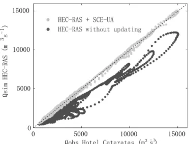
Figure 8 shows a scatter plot between calculated and observed
values along the optimization window, with and without HEC-RAS model updating. To ignore calculated lows during both model warmup (0-72 h) and irst intervals in the optimization window (73 h-108 h), since the latter is much penalized by the weight
function w(t), only values for the interval between 108 h and 144 h were plotted corresponding to the second half of this window.
When the hydraulic model is run without updating, the
tendency of underestimation increases for higher lows, while
farthest points of the perfect prediction (45º dashed line) may be
related to higher low contributions from tributaries. In addition, the loop-shaped curve can be mainly explained by lag errors
associated to the hydraulic model. It happens because obtaining
accurate results of discharge for both high and low low conditions is dificult, especially when the model is calibrated with river stage
and geometry of the cross sections is complemented by SRTM
data. Nevertheless, when HEC-RAS updating is performed, it can be clearly seen that model simulations almost it the observed lows
over the optimization window, accounting for errors originating from different sources of uncertainty.
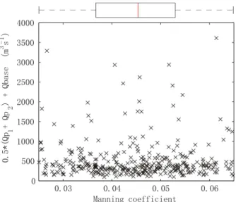
To assess the behavior of decision variables and characteristics
of the estimated lateral inlows, Figures 9 and 10 show the parameters
related to streamlow plotted against the displacement parameter and the Manning coeficient, respectively. In these diagrams, the
average between Qp1 and Qp2 summed to Qbase is related to the
magnitude of the lateral inlow, while the absolute difference
between td1 and td2 indicates the distance between peaks of both resulting hydrographs. Regarding the displacement parameter, a
concentration of points near the origin of x-axis shows that the
Table 3. Performance of the coupling algorithm and estimated
variables for each SCE-UA coniguration.
Param. / SCE-UA
conf. 1 2 3
HEC-RAS runs 801 1890 4433
Processing time 36 min 68 min 158 min
Td1 24.9 24.8 24.7
Td2 24.8 24.7 25.0
Qp1 161.8 214.6 217.3
Qp2 252.1 202.6 193.7
Qbase 340.5 338.8 341.9
Manning coeff. 0.043 0.036 0.051
FO 148442 148462 148603
Table 1. Minimum and maximum limits for SCE-UA decision variables.
Parameter Qbase Manning td1 Qp1 td2 Qp2
Min. value 0 0.025 -10 0 -10 0
Max. value 4000 0.065 52 3000 52 3000
Table 2. SCE-UA setups for the convergence test.
Conig. complexes n. (c)
n. points in
complex
(p)
n. solutions
(NS)
n. generations
(NG)
1 3 7 21 20
2 7 10 70 20
3 11 13 143 30
in an global optimum, since a given combination of lateral inlow
parameters (td, Qp and Qbase) offsets the lack of representativeness
of Manning coeficient. Therefore, adopting a large search space
for this parameter may be inadequate, precisely by making the
updating method more susceptible to an equiinality problem
(BEVEN, 2006).
In order to assess the beneit of HEC-RAS updating for operational streamlow forecasting, the Nash-Sutcliffe eficiency (NSE) (Figure 11), the mean absolute error (MAE) and the mean relative error (MRE) (Figure 12) were plotted for different forecast lead times. Results were separated according to the 10% value of
the low duration curve (Q10 = 3580 m3s-1), so that performance can
be evaluated for lows exceeding and not exceeding the Q10 value.
When model is run without updating, all metrics have an
approximately sinusoidal behavior for lows below Q10 threshold,
whereas model performance is better for longer lead times. This occurs because most of the forecasts started during the rise of the hydrograph generated by the daily operation cycle of Salto
lateral inlow was unimodal in many cases, but the associated lows were often relatively small. This is not much expected, since the
sum of peaks in very close intervals would be more appropriate to
account for major underestimation, i.e., during high low periods.
Moreover, it can be noticed that the predominant distances between
the peaks ranged between 20 and 35 hours. Considering the rise
time adopted for the case study (Tp = 20 hours), distances close to or above this value would indicate a bimodal lateral hydrograph occurring in most part of the time.
In relation to the Manning coeficient, it is clear that the
SCE-UA algorithm found possible solutions in the whole search
space. For lateral inlows with lower magnitude, the roughness values were well distributed within minimum and maximum limits.
Although with a fewer number of points, this tendency can be
also noticed for high lows, and in cases where the lateral inlow exceeded 3000 m3s-1, Manning coeficients were either less than
0.030 or greater than 0.060. This behavior indicates that a solution
composed by a less physical meaning of roughness can also result
Figure 8. Scatter plot between observed and simulated lows along the optimization window (t = 108 to 144 h). Dashed line indicates the perfect prediction.
Caxias reservoir, as well as by a delay in lows calculated by the hydraulic model (lag error). Thus, low underestimation reach maximum values at the peak of observed hydrograph (irst lead
times) and reduce during its recession (longer lead times), since
predicted lows are still rising during the latter period. For lows exceeding the Q10 threshold, results without model updating are in agreement with the ones by Meller, Bravo and Collischonn (2012) where model performance hardly varies in forecast range. This is
explained by the fact that no modiication of the initial conditions
is conducted prior to the forecast and because there is little or
no inluence of the daily operation cycle for this range of lows.
By the other hand, it is noteworthy that updating of
HEC-RAS model had a very positive impact on the performance of streamlow forecast, accounting for both underestimation and lag errors in model computations. Performance is maximum in the
start of forecast and gradually reduces when lead time is increased,
which is somehow expected since the recession of lateral inlow
hydrograph occurs during the forecast range. Figure 10. Relationship between Manning coeficient and low
parameters in estimated lateral inlows.
Figure 11. Nash-Sutcliffe eficiency for each forecast lead time, with and without HEC-RAS model updating.
Figure 13 shows some graphical examples of the HEC-RAS model updating using the SCE-UA algorithm. The lateral inlow
generated with only two synthetic hydrographs offers a good
agreement between observed and simulated lows to a suficient
number of time intervals. According to the illustrations (a), (c) and
(e) the contribution of tributaries between Salto Caxias reservoir and Hotel Cataratas can be quite considerable, demonstrating that introducing a lateral inlow in this reach is critical to reduce
model underestimation for streamlow forecasting. Illustrations
(b) and (d) show situations in which the updating procedure
improves the forecast of an isolated peak, and are examples where the lateral inlow parameters offset a relatively high value of Manning coeficient.
Finally, in the illustration (f) the updating procedure is applied
during a lood situation, when lows of Iguazu river are starting to exceed the channel capacity. Thus, the observed hydrograph has
a delayed peak compared with the simulated one due to a slight
loodplain attenuation, which is poorly represented in HEC-RAS
model since SRTM data is used as a complementary information
to geometry. In this case, the lateral inlow hydrograph is closer to the left side of optimization window to account for higher low
differences in the intermediate time intervals, which had a great
impact on the objective function. The beneit of model updating
in the forecast range was lower if compared with the other cases, which could be improved by adjustments in the weight function w(t).
CONCLUDING REMARKS
Recent technological advances and development of software packages have been facilitating the preparation of hydrodynamic models for solving a variety of water resources problems. When it comes to operational hydrological forecasting, where challenges
still remain by either complexity of assimilation techniques or
preference for robust and easily handled models, the widely known computational tools can be very useful to overcome these limitations especially when combined with simpler methods of real time model updating.
In this work, we presented a real-time HEC-RAS updating procedure for streamlow forecasting using the SCE-UA optimization algorithm. For its evaluation, an existing HEC-RAS model for
Iguazu river, a tributary of Parana river right after the Itaipu dam, was used as a study case. Results showed that differences between simulated and observed discharges can be reduced with the application of SCE-UA algorithm, which proved to be
effective when used with a relatively small number of complexes
and solutions. The updating procedure improved the performance
of HEC-RAS for predicting lows, also reducing negative effects caused by lag errors in the hydraulic model. However, it is important
to note that the algorithm does not differentiate between a more physically consistent solution to other hardly found in the real world. This means that the parameters obtained for the lateral
inlow may offset a low or high value of Manning coeficient (for
instance, n = 0.06 for the river channel in the latter case), which requires a more suitable search space for the roughness parameter.
The methodology presented herein shows that it is
possible to update a widely known model such as the HEC-RAS for real-time streamlow forecasting, taking full advantage of a previously calibrated model as well as the experience of the
users. Automation of the hydraulic model reduces both the need
for excessive manipulation of iles and manual adjustments in
the model itself, which presents as a major advantage when important decisions must be taken in a relatively short time. In the
Brazilian context, where reservoir operation is essential for both energy production and lood control, similar procedures could be
developed for other purposes, such as opening and closing gates
for meeting local constraints based on predicted reservoir inlow.
ACKNOWLEDGEMENTS
The irst author would like to acknowledge the National Counsel of Technology and Scientiic Development (CNPQ) and
the anonymous reviewers who contributed for the improvement of this manuscript.
REFERENCES
ADAMS, T.; CHEN, S.; HEIM, J. NWS/OHRFC Operational
Experience with the Ohio River Community HEC-RAS Model. In: WORLD ENVIRONMENTAL AND WATER RESOURCES CONGRESS, 11., 2011. Palm Springs. Proceedings… Palm Springs: ASCE, 2011. p. 2244-2252.
ARAUJO, A. N.; BREDA, A.; FREITAS, C.; LEITE, E. A.;
GONÇALVES, J. E.; CALVETTI, L.; ALMEIDA, M. I.; SILVEIRA,
R. B. Hydrological and meteorological forecast combined systems
for flood alerts and reservoir management: the Iguaçu river basin
case. In: INTERNATIONAL CONFERENCE IN FLOOD MANAGEMENT, 6., 2014. São Paulo. Proceedings… São Paulo:
ABRH, 2014. Available from: <http://www.abrh.org.br/icfm6/
proceedings/papers/PAP014749.pdf>. Access on: 10 july 2016.
AYVAZ, M. T. A linked simulation-optimization model for simultaneously estimating the manning roughness in shallow water flows. Journal of Hydrology, v. 500, p. 183-199, 2013. http://
dx.doi.org/10.1016/j.jhydrol.2013.07.019.
BABOVIC, V.; CANIZARES, R.; JENSEN, H. R.; KLINTING,
A. Neural networks as routine for error updating of numerical
models. Journal of Hydraulic Engineering, v. 127, n. 3, p. 181-193, 2001.
http://dx.doi.org/10.1061/(ASCE)0733-9429(2001)127:3(181).
BASHIRI-ATRABI, H.; QADERI, K.; RHEINHEIMER, D. E.; SHARIFI, E. Application of harmony search algorithm to reservoir operation optimization. Water Resources Management, v. 29, n. 15, p. 5729-5748, 2015. http://dx.doi.org/10.1007/
s11269-015-1143-3.
BEVEN, K. A manifesto for the equifinality thesis. Journal of Hydrology, v. 320, n. 1-2, p. 18-36, 2006.
BRAVO, J. M.; ALLASIA, D.; PAZ, A. R.; COLLISCHONN, W.; TUCCI, C. E. M. Coupled hydrologic-hydraulic modeling of the Upper Paraguay river basin. Journal of Hydrologic Engineering,
v. 17, n. 5, p. 635-646, 2012. http://dx.doi.org/10.1061/(ASCE) HE.1943-5584.0000494.
BRAVO, J. M.; COLLISCHONN, W.; TUCCI, C. E. M.; PILLAR, J. V. Otimização de regras de operação de reservatórios com incorporação da previsão de vazão. Revista Brasileira de Recursos Hídricos, v. 13, n. 1, p. 181-196, 2008. http://dx.doi.org/10.21168/
rbrh.v13n1.p181-196.
BREDA, A.; GONÇALVES, J. E.; SILVEIRA, R. B. Análise
de alterações em componentes de um método de calibração automática mono-objetivo na qualidade e eficiência de ajuste de parâmetros do Modelo Sacramento. Revista Brasileira de Recursos Hídricos, v. 16, n. 2, p. 89-100, 2011. http://dx.doi.org/10.21168/ rbrh.v16n2.p89-100.
baseada no modelo SMAP e com incorporação de informações
de precipitação. Revista Brasileira de Recursos Hídricos, v. 12, n. 3, p. 57-68, 2007. http://dx.doi.org/10.21168/rbrh.v12n3.p57-68.
CESTARI JUNIOR, E.; SOBRINHO, M. D.; OLIVEIRA, J.
N. Estudo de propagação de ondas para auxiliar a elaboração do Plano de Ação Emergencial Externo - PAE. Revista Brasileira de Recursos Hídricos, v. 20, n. 3, p. 689-697, 2015. http://dx.doi.
org/10.21168/rbrh.v20n3.p689-697.
CHE, D.; MAYS, L. W. Development of an optimization/simulation model for real-time flood-control operation of river-reservoirs systems. Water Resources Management, v. 29, n. 11, p. 3987-4005, 2015. http://dx.doi.org/10.1007/s11269-015-1041-8.
CLOKE, H. L.; PAPPENBERGER, F. Ensemble flood forecasting: A review. Journal of Hydrology, v. 375, n. 3-4, p. 613-626, 2009.
http://dx.doi.org/10.1016/j.jhydrol.2009.06.005.
DEMARIA, E. M. C.; NIJSSEN, B.; VALDÉS, J. B.; RODRIGUEZ, D. A.; SU, F. Satellite precipitation in southeastern South America:
How do sampling errors impact high flow simulations? International Journal of River Basin Management, v. 12, n. 1, p. 1-14, 2014. http://
dx.doi.org/10.1080/15715124.2013.865637.
DOMENEGHETTI, A.; CASTELLARIN, A.; BRATH, A. Assessing rating-curve uncertainty and its effects on hydraulic model calibration. Hydrology and Earth System Sciences, v. 16, n. 4, p. 1191-1202, 2012. http://dx.doi.org/10.5194/hess-16-1191-2012.
DUAN, Q.; SOROOSHIAN, S.; GUPTA, V. Effective and efficient global optimization for conceptual rainfall-runoff models. Water Resources Research, v. 28, n. 4, p. 1015-1031, 1992.
http://dx.doi.org/10.1029/91WR02985.
FARR, T. G.; CARO, E.; CRIPPEN, R.; DUREN, R.; HENSLEY, S.; KOBRICK, M.; PALLER, M.; RODRIGUEZ, E.; ROSEN, P.;
ROTH, L.; SEAL, D.; SHAFFE, R. S.; SHIMADA, J.; UMLAND, J.; WERNER, M.; BURBANK, D.; OSKIN, M.; ALSDORF, D. The shuttle radar topography mission. Reviews of Geophysics, v. 45, n. 2, p. RG2004, 2007. http://dx.doi.org/10.1029/2005RG000183.
FERREIRA, L. R. A.; SOARES FILHO, S. Modelo de simulação em base horária da vazão na estação fluviométrica da régua-11. In: SIMPÓSIO BRASILEIRO DE SISTEMAS ELÉTRICOS,
4., 2012, Goiânia. Anais... Goiânia: UFG, 2012. v. 1. p. 1-6.
FIGUEIREDO, K.; BARBOSA, C. R. H.; CRUZ, A. V. A.; VELLASCO, M.; PACHECO, M. A. C.; CONTRERAS, R. J.; BARROS, M.; SOUZA, R. C.; MARQUES, V. S.; DUARTE, U. M.; MENDES, M. H. Modelo de previsão de vazão com informação de precipitação utilizando redes neurais. Revista Brasileira de Recursos Hídricos, v. 12, n. 3, p. 69-82, 2007. http://
dx.doi.org/10.21168/rbrh.v12n3.p69-82.
GOODELL, C. R. Breaking the HEC-RAS code: a user guide to
automating HEC-RAS. Portland: H2ls, 2014. 278 p.
GUILHON, L. G. F.; ROCHA, V. F.; MOREIRA, J. C.
Comparação de métodos de previsão de vazões naturais afluentes
a aproveitamentos hidrelétricos. Revista Brasileira de Recursos Hídricos, v. 12, n. 3, p. 13-20, 2007. http://dx.doi.org/10.21168/
rbrh.v12n3.p13-20.
HABERT, J.; RICCI, S.; LE PAPE, E.; THUAL, O.; PIACENTINI, A.; GOUTAL, N.; JONVILLE, G.; ROCHOUX, M. Reduction of the uncertainties in the water level-discharge relation of
a 1D hydraulic model in the context of operational flood
forecasting. Journal of Hydrology, v. 532, p. 52-64, 2016. http://
dx.doi.org/10.1016/j.jhydrol.2015.11.023.
HICKS, F. E.; PEACOCK, T. Suitability of HEC-RAS for flood forecasting. Canadian Water Resources Journal, v. 30, n. 2, p. 159-174, 2005. http://dx.doi.org/10.4296/cwrj3002159.
HSU, M.-H.; FU, J.-C.; LIU, W.-C. Flood routing with real-time stage correction method for flash flood forecasting in the Tanshui River, Taiwan. Journal of Hydrology, v. 283, n. 1-4, p. 267-280, 2003.
http://dx.doi.org/10.1016/S0022-1694(03)00274-9.
HSU, M.-H.; FU, J.-C.; LIU, W.-C. Dynamic routing model with real-time roughness updating for flood forecasting. Journal of Hydraulic Engineering, v. 132, n. 6, p. 605-619, 2006. http://dx.doi.
org/10.1061/(ASCE)0733-9429(2006)132:6(605).
HEC – HYDROLOGIC ENGINEERING CENTER; USACE – U.S. ARMY CORPS OF ENGINEERS. HEC-RAS hydraulic reference manual, version 4.1. Davis: Institute of Water Resources,
Hydrological Engineering Center, 2010.
LEON, A.; GOODELL, C. Controlling HEC-RAS using MATLAB. Environmental Modelling and Software, v. 84, n. 10, p.
339-348, 2016. http://dx.doi.org/10.1016/j.envsoft.2016.06.026.
LIU, Y.; WEERTS, A. H.; CLARK, M.; HENDRICKS
FRANSSEN, H.-J.; KUMAR, S.; MORADKHANI, H.; SEO, D.-J.; SCHWANENBERG, D.; SMITH, P.; VAN DIJK, A. I. J. M.;
VAN VELZEN, N.; HE, M.; LEE, H.; NOH, S. J.; RAKOVEC, O.; RESTREPO, P. Advancing data assimilation in operational hydrologic forecasting: progresses, challenges, and emerging opportunities. Hydrology and Earth System Sciences, v. 16, n. 10, p.
3863-3887, 2012. http://dx.doi.org/10.5194/hess-16-3863-2012.
MADSEN, H.; SKOTNER, C. Adaptive state updating in real time river flow forecasting - A combined filtering and error forecasting procedure. Journal of Hydrology, v. 308, n. 1-4, p.
302-312, 2005. http://dx.doi.org/10.1016/j.jhydrol.2004.10.030.
MALEKMOHAMMADI, B.; KERACHIAN, R.; ZAHRAIE, B. A real-time operation optimization model for flood management in river-reservoir systems. Natural Hazards, v. 53, n. 3, p. 459-482, 2010. http://dx.doi.org/10.1007/s11069-009-9442-8.
Potomac: evaluation for freshwater, tidal and wind-driven elements. Journal of Hydraulic Engineering, v. 140, n. 5, p. 04014005, 2014.
http://dx.doi.org/10.1061/(ASCE)HY.1943-7900.0000862.
MASKEY, S.; GUINOT, V.; PRICE, R. K. Treatment of precipitation uncertainty in rainfall-runoff modeling: a fuzzy set approach. Advances in Water Resources, v. 27, n. 9, p. 889-898, 2004. http://dx.doi.org/10.1016/j.advwatres.2004.07.001.
MEDIERO, L.; GARROTE, L.; CHAVEZ-JIMENEZ, A. Improving probabilistic flood forecasting through a data assimilation scheme based on genetic programming. Natural Hazards and Earth System Sciences, v. 12, n. 12, p. 3719-3732, 2012.
http://dx.doi.org/10.5194/nhess-12-3719-2012.
MELLER, A.; BRAVO, J. M.; COLLISCHONN, W. Assimilação de dados de vazão na previsão de cheias em tempo real com
o modelo hidrológico MGB-IPH. Revista Brasileira de Recursos Hídricos, v. 17, n. 3, p. 209-224, jul./set. 2012.
MONTE, B. E. O.; COSTA, D. D.; CHAVES, M. B.; MAGALHÃES, L.; UVO, C. O.; UVO, C. B. Hydrologic and Hydraulic modeling applied to the mapping of flood-prone areas. Revista Brasileira de Recursos Hídricos, v. 21, n. 1, p. 152-167, 2016. http://dx.doi. org/10.21168/rbrh.v21n1.p152-167.
MOREDA, F.; GUTIERREZ, A.; REED, S.; ASCHWANDEN,
C. Transitioning NWS operational hydraulics models from FLDWAV to HEC-RAS. In: WORLD ENVIRONMENTAL AND WATER RESOURCES CONGRESS, 1., 2009, Kansas. Proceedings... Reston: ASCE, 2009. p. 1-11
NEAL, J. C.; ATKINSON, P. M.; HUTTON, C. W. Flood
inundation model updating using Ensemble Kalman filter
and spatially distributed measurements. Journal of Hydrology,
v. 336, n. 3-4, p. 401-415, 2007. http://dx.doi.org/10.1016/j.
jhydrol.2007.01.012.
NELDER, J. A.; MEAD, R. A simplex method for function minimization. The Computer Journal, v. 7, n. 4, p. 308-313, 1965.
http://dx.doi.org/10.1093/comjnl/7.4.308.
NGO, L. L.; MADSEN, H.; ROSBJERG, D. Simulation and
optimization modeling approach for operation of the Hoa Binh
reservoir, Vietnam. Journal of Hydrology, v. 336, n. 3-4, p. 269-281, 2007. http://dx.doi.org/10.1016/j.jhydrol.2007.01.003.
NRCS - NATIONAL RESOURCES CONSERVATION SERVICES; USDA - UNITED STATES DEPARTMENT OF AGRICUTURE. Hydrographs. In: NRCS - NATIONAL
RESOURCES CONSERVATION SERVICES; USDA - UNITED STATES DEPARTMENT OF AGRICUTURE. National Engineering Handbook Hydrology. Washington: NRCS/USDA, 2007. chap. 16.
O’CONNEL, P.; CLARKE, R. T. Adaptive hydrological forecasting - a review. Hydrological Sciences Bulletin, v. 26, n. 2, p. 179-205, 1981. http://dx.doi.org/10.1080/02626668109490875.
PAIVA, R. C. D.; COLLISCHONN, W.; TUCCI, C. E. M. Large scale hydrologic and hydrodynamic modeling using limited data and a GIS based approach. Journal of Hydrology, v. 406, n. 3-4, p. 170-181, 2011. http://dx.doi.org/10.1016/j.jhydrol.2011.06.007.
PAPPENBERGER, F.; BEVEN, K.; HORRIT, M. S.; BLAZKOVA, S. D. Uncertainty in the calibration of effective roughness
parameters in HEC-RAS using inundation and downstream
level observations. Journal of Hydrology (Amsterdam), v. 302, n. 1, p. 46-69, 2005. http://dx.doi.org/10.1016/j.jhydrol.2004.06.036.
PAZ, A. R.; BRAVO, J. M.; ALLASIA, D.; COLLISCHONN, W.; TUCCI, C. E. M. Large-scale hydrodynamic modeling of
a complex river network and floodplains. Journal of Hydrologic Engineering, v. 15, n. 2, p. 1-15, 2010. http://dx.doi.org/10.1061/
(ASCE)HE.1943-5584.0000162.
PAZ, A. R.; COLLISCHONN, W.; TUCCI, C. E. M.; CLARKE, R. T.; ALLASIA, D. Data assimilation in a large-scale distributed hydrological model for medium-range flow forecasts. In:
PROCEEDINGS OF SYMPOSIUM HS2004 AT IUGG2007, 1., 2007, Perugia. Perugia: IAHS, 2007. p. 471-478.
REFSGAARD, J. C. Validation and intercomparison of different updating procedures for real-time forecasting. Nordic Hydrology, v. 28, n. 2, p. 65-84, 1997.
REYNAUD, F.; MINE, M. R. M.; KAVISKI, E. Aplicação do modelo de Skaugen para desagregação espacial da chuva no rio Iguaçu. Revista Brasileira de Recursos Hídricos, v. 19, n. 3, p. 97-110, 2014. http://dx.doi.org/10.21168/rbrh.v19n3.p97-110.
RIBEIRO NETO, A.; CIRILO, J. A.; DANTAS, C. E. O.; SILVA, E. R. Caracterização da formação de cheias na bacia do rio Una
em Pernambuco: simulação hidrológica-hidrodinâmica. Revista Brasileira de Recursos Hídricos, v. 20, n. 2, p. 394-403, 2015. http://
dx.doi.org/10.21168/rbrh.v20n2.p394-403.
RICCI, S.; PIACENTINI, A.; THUAL, O.; LE PAPE, E.;
JONVILLE, G. Correction of upstream flow and hydraulic
state with data assimilation in the context of flood forecasting.
Hydrology and Earth System Sciences, v. 15, n. 11, p. 3555-3575, 2011.
http://dx.doi.org/10.5194/hess-15-3555-2011.
ROMANOWICZ, R. J.; YOUNG, P. C.; BEVEN, K. J.;
PAPPENBERGER, F. A data based mechanistic approach to nonlinear flood routing and adaptive flood level forecasting. Advances in Water Resources, v. 31, n. 8, p. 1048-1056, 2008. http://
dx.doi.org/10.1016/j.advwatres.2008.04.015.
SANTOS, C. A. G.; SUZUKI, K.; WATANABE, M. Modificação no Algoritmo Genético SCE-UA e sua Aplicação a um Modelo
Hidrossedimentológico. Revista Brasileira de Recursos Hídricos, v. 8,
0b5ac061c155886_90f24e2aeee68f5ce4bd81a76e7bf182.pdf>.
Access on: 30 apr. 2016.
WU, X.-L.; XIANG, X.-H.; WANG, C.-H.; CHEN, X.; XU,
C.-Y.; YU, Z. Coupled hydraulic and Kalman filter model for
real-time correction of flood forecast in the three gorges interzone
of Yangtze river, China. Journal of Hydrologic Engineering, v. 18,
n. 11, p. 1416-1425, 2013. http://dx.doi.org/10.1061/(ASCE) HE.1943-5584.0000473.
YANG, T.-H.; WANG, Y.-C.; TSUNG, S.-C.; GUO, W.-D. Applying micro-genetic algorithm in the one-dimensional unsteady hydraulic model for parameter optimization. Journal of Hydroinformatics, v. 16, n. 4, p. 772-783, 2014. http://dx.doi.
org/10.2166/hydro.2013.030.
ZAPPA, M.; JAUN, S.; GERMANN, U.; WALSSER, A.; FUNDEL, F. Superposition of three sources of uncertainties in operational flood forecasting chains. Atmospheric Research, v. 100, n. 2-3, p. 246-262, 2011. http://dx.doi.org/10.1016/j.atmosres.2010.12.005.
Authors contributions
Vinícius Alencar Siqueira: Development of coupling algorithm,
literature review, data processing and simulations, generation
and assessment of results, text organization and writing of the
manuscript.
Mino Viana Sorribas: Literature review and detailed paper review.
Juan Martin Bravo: Development of SCE-UA algorithm and paper review.
Walter Collischonn: Initial draft of the updating method and paper review.
Auder Machado Vieira Lisboa: HEC-RAS model supply and
paper review.
Giovanni Gomes Villa Trinidad: HEC-RAS model supply and