i
Continuum Modelling and Numerical Simulation of Damage for
Ductile Materials
Dissertation presented to the Faculty of Engineering, University of Porto, as a requirement to obtain the Ph.D. degree in Mechanical Engineering, carried out under the supervision of Professor Francisco Manuel Andrade Pires, Associate Professor, Faculty of Engineering, University of Porto and Professor José Manuel de Almeida César de Sá, Full Professor, Faculty of Engineering, University of Porto
Lucival Malcher
Faculdade de Engenharia Universidade do Porto
Porto
iii
v
AGRADECIMENTOS
Em primeiro lugar, gostaria de agradecer o apoio dado pelo meus orientadores Dr. Francisco Manuel de Andrade Pires e Dr. José César de Sá, durante o desenvolvimento deste trabalho e principalmente pela oportunidade de ter feito este doutoramento na FEUP. Gostaria de agradecer também a Fundação para a Ciência e Tecnologia - FCT, pelo apoio financeiro dado.
Agradecimentos especiais vão também aos colegas de estudo e grandes amigos Dr. Filipe Xavier Costa Andrade, Dr. Thiago Doca e Dr. Fabio José Pinho Reis. Obrigado pelo apoio, conversas, discussões e pela grande troca de experiência e influência no tema deste trabalho. Agradeço o sempre apoio do Professor Dr. José Carlos Balthazar, da Universidade de Brasília, que foi meu orientador tanto durante minha graduação quanto no mestrado concluído na UnB.
Agradeço à minha mãe (Graça Malcher Ávila) e pai (Antonio Ávila) pelo grande incentivo em levar estes estudos com garra até o seu fim.
Por fim, meus maiores agradecimentos vão para minha esposa Cyntia de Souza Malcher, que acreditou no meu sonho e vontade de seguir estes estudos fora de nosso conforto e país.
vii
RESUMO
A correta determinação da fratura em materiais dúcteis tem avançado enormemente nos últimos anos e assim, o aperfeiçoamento de novas formulações e técnicas que sejam capazes de melhorar o comportamento preditivo de modelos constitutivos tornou-se um grande objeto de estudo para pesquisadores em todo o mundo. O avanço da indústria e a procura de técnicas que possibilitem o aumento da competitividade, fez com que tais desenvolvimentos acadêmicos passassem a ser adotados por inúmeros setores como o automobilístico, o aeroespacial, o naval, entre outros. Desta forma, nesta tese, procura-se contribuir para o desenvolvimento e aperfeiçoamento de modelos constitutivos e numéricos que sejam capazes de determinar, da maneira mais realística possível, o comportamento mecânico de materiais metálicos. Para isto, como primeira etapa do trabalho, sugere-se um algoritmo de integração numérica implícita para um modelo elasto-plástico avançado, que inclui a influência da pressão hidrostática e do terceiro invariante do tensor desviador, na lei de fluxo plástico de um material metálico. Após esta proposição, busca-se avaliar o comportamento preditivo de três formulações constitutivas disponíveis na literatura para determinação do correto local e momento de início de uma fenda dúctil. São então avaliados, o modelo de Bai e Wierzbicki, o modelo de Lemaitre e o modelo de Gurson em uma versão modificada e conhecida por GTN. Como etapa seguinte desta tese, procurou-se avaliar o desempenho de dois mecanismos de corte, um proposto por Xue e outro por Nahshon et al., acoplados ao modelo GTN e aplicados à região de baixa triaxialidade. Nesta etapa, avaliou-se a influência da relação entre a condição de calibração dos parâmetros materiais e a condição de uso, na capacidade preditiva dos modelos com variáveis interna de dano acoplada. Com base nos resultados observados, na etapa seguinte, propõe-se um novo modelo constitutivo, baseado na formulação de Gurson e na dedução geométrica da lei de evolução do mecanismo de corte de Xue, de maneira a aumentar a capacidade preditiva no que se refere a: determinação do nível esperado de deformação plástica equivalente na fratura, o nível de deslocamento na fratura e o potencial local para início da fratura dúctil, bem como reduzir a influência do ponto de calibração na precisão dos resultados numéricos obtidos quando o modelo é aplicado a largas faixas de triaxialidade. Por fim, o modelo desenvolvido com base na teoria de Gurson, que agora passa a denominar de "extended GTN model", é testado em condições complexas de carregamento, com o intuito de se avaliar a influência da história do carregamento no comportamento mecânico de materiais e a capacidade preditiva do modelo. Para isto, introduz-se o efeito de Bauschinger no modelo, através do acoplamento da lei de fluxo plástico com uma lei de endurecimento cinemático, como proposto por Prager.ix
ABSTRACT
Accurate determination of fractures in ductile materials has improved significantly in recent years, and so the development of new formulations and techniques to improve the performance of predictive constitutive models has become a major topic of study for researchers worldwide. Industry progress and demand for techniques that allow for increased competitiveness caused such academic developments to spread into numerous industries, such as the automotive, aerospace and shipbuilding sectors, among others. Thus, this thesis seeks to contribute to the development and refinement of constitutive and numerical models to determine the mechanical behavior of metallic materials as realistically as possible. To this end, the first step is to propose an implicit numerical integration algorithm for an advanced elasto-plastic model, which includes the influence of hydrostatic pressure and third invariant of deviator tensor on the plastic flow rule for a metallic material. Once this proposition has been made, the predictive performance of three constitutive formulations available in the literature are analyzed for determining the exact place and time of development of a ductile crack. The Bai and Wierzbicki model, the Lemaitre model and the Gurson model are then evaluated in a modified version known as GTN. The next step in this thesis was to evaluate the performance of two shear mechanisms – a mechanism proposed by Xue and another mechanism proposed by Nahshon et al., coupled with the GTN model and applied to the range of low stress triaxiality. In this step, the influence of the relationship between the calibration condition material parameters and use condition was evaluated with regard to the predictive ability of the models with coupled internal damage variables. Based on the results, in the following step a new constitutive model is proposed that is based on Gurson’s formulation and the geometric deduction of Xue’s evolution law for the shear mechanism so as to increase predictive ability with respect to: determining the expected level of equivalent plastic strain at fracture, the level of displacement at fracture and the local potential for development of a ductile fracture, as well as reducing the influence of the calibration point on the accuracy of numerical results obtained when the model is applied to wide range of stress triaxiality. Finally, the model based on Gurson’s theory – now called the “extended GTN model” – is tested under complex loading conditions in order to evaluate the influence of the loading history on the mechanical behavior of materials and predictive ability of the model. To this end, the Bauschinger effect is introduced in the model by coupling the plastic flow rule with a kinematic hardening law as proposed by Prager for the evolution of the back stress.xi
CONTENTS
AGRADECIMENTOS v RESUMO vii ABSTRACT ix CONTENTS xi 1. INTRODUCTION 1 1.1 General Considerations 11.2 Importance and Evolution of The Continuun Damage Mechanics 3
1.3 Layout 4
2. CONTINUUM MECHANICS, LAWS OF THERMODYNAMICS AND CONSTITUTIVE
THEORY 7
2.1 Kinematics Of Deformation 7
2.1.1 Configurations and motions of continuum bodies 7
2.1.2 Material and spatial descriptions 10
2.1.3 The deformation gradient 11
2.1.4 Polar decomposition: Stretches and rotation 14
2.1.5 Strain Measures 15
2.1.6 The velocity gradient: Rate of deformation and spin 16 2.1.7 Superimposed rigid body motions and objectivity 17
2.2 Stress and Equilibrium 18
2.2.1 The Cauchy stress tensor 19
2.2.2 Alternative stress tensors 20
2.3 Fundamental Laws of Thermodynamics 21
2.3.1 Conservation of mass 21
2.3.2 Momentum balance 22
2.3.3 The first principle 22
2.3.4 The second principle 23
2.3.5 The Clausius-Duhem inequality 23
2.4 Constitutive Theory 23
2.4.1 Thermodynamics with internal variables 24
2.4.2 Phenomenological and micromechanical approaches 27
2.4.3 The purely mechanical theory 28
2.4.4 The constitutive initial value problem 28
2.5 Weak Equilibrium. The Principle of Virtual Work 29
2.5.1 The spatial version 29
xii
3. AN IMPLICIT NUMERICAL INTEGRATION ALGORITHM FOR AN ELASTO-PLASTIC
MODEL WITH THREE INVARIANTS 31
3.1 Introduction 32
3.2 Preliminaries 33
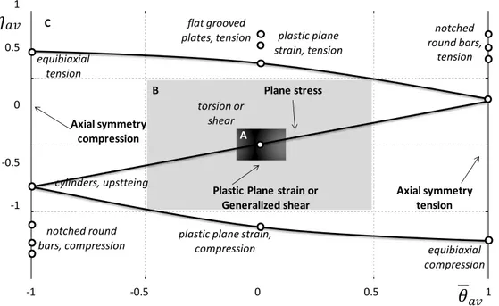
3.2.1 Lode Angle Parameter 34
3.2.2 Fracture Surface 35
3.3 Constitutive Model 37
3.4 Numerical Strategy for The Integration Algorithm 41
3.4.1 State update procedure 42
3.4.2 Accuracy and stability 49
3.4.3 Consistent tangent operator 52
3.4.4 Convergence of the equilibrium problem 53
3.5 Numerical Simulation 55
3.5.1 Geometry and mesh definition 55
3.5.2 Numerical results 58
3.6 Conclusions 65
4. AN ASSESSMENT OF ISOTROPIC CONSTITUTIVE MODELS FOR DUCTILE
FRACTURE UNDER HIGH AND LOW STRESS TRIAXIALITY 67
4.1 Introduction and Motivation 68
4.2 Constitutive Models for Ductile Fracture 72
4.2.1 The Gurson-Tvergaard-Needleman Model 72
4.2.1.1 Shear Mechanism 75
4.2.2 Lemaitre’s Damage Model 78
4.2.3 Bai & Wierzbicki Model 81
4.3 Numerical Solution Strategy 81
4.4 Numerical Examples 87
4.4.1 General Information 87
4.4.2 Geometry and Mesh Definition 89
4.4.3 Calibration of Material Parameters for 2024-T351 Al 94
4.5 Numerical Results 96
4.5.1 High Stress Triaxiality (1⁄3≤η<1) 97
4.5.2 Low Stress Triaxiality (0≤η<1⁄3) 107
4.5.3 Discussion 115
4.5.4 Fracture Locus Representation 118
4.5 Conclusions 119
5. NUMERICAL TEST FOR SHEAR MECHANISMS AND INFLUENCE OF THE CALIBRATION POINT ON THE NUMERICAL RESULTS FOR COUPLED DAMAGE
MODELS: BASED ON GTN MODEL 121
5.1 Introduction 122
5.2 Constitutive Model 123
5.2.1 Gurson-Tvergaard-Needleman (GTN)'s model 127
5.2.2 Shear Mechanisms 128
5.2.3 Lode Angle Function 134
5.3 Numerical Integration Algorithm 136
xiii
5.4 Calibration Procedure 140
5.4.1 Inverse method for parameter identification 141
5.4.2 Geometry and mesh definition 143
5.4.3 First Calibration Point: smooth bar specimen (tensile loading test) 144 5.4.4 Second Calibration Point: butterfly specimen (shear loading test) 146
5.5 Numerical Results 147
5.5.1 Equivalent plastic strain at fracture 149
5.5.2 Evolution of damage parameter 150
5.5.3 Determination of fracture onset 155
5.6 Conclusions 158
6. AN EXTENDED GTN MODEL FOR DUCTILE FRACTURE UNDER HIGH AND LOW
STRESS TRIAXIALITY 159
6.1 Introduction 160
6.2 Extended Constitutive Formulation 161
6.2.1 Nucleation mechanism 161
6.2.2 Incorporation of Shear Effects 163
6.2.3 Damage Evolution 165
6.2.4 Modified Lode Angle Dependence Function 167
6.2.5 Coalescence Criterion 171
6.3 Numerical Integration Algorithm 175
6.3.1 The Elastic Trial Step 175
6.3.2 The Plastic Corrector Step or Return Mapping Algorithm 176
6.3.3 The Consistent Tangent Operator 183
6.4 Calibration Procedure 185
6.4.1 Geometry and mesh definition 185
6.4.2 First Calibration Point: smooth bar under tensile loading condition 188 6.4.3 Second Calibration Point: pure shear loading condition 190
6.5 Numerical Results 191
6.5.1 Evolution of equivalent plastic strain and damage parameters 192 6.5.2 Prediction of the correct fracture location 199 6.5.3 Representation in the three dimensional fracture locus 201
6.6 Conclusions 202
7. AN ENHANCED MICROMECHANICAL CONSTITUTIVE MODEL FOR THE
PREDICTION OF THE LOADING HISTORY EFFECT WITH DUCTILE FRACTURE 205
7.1 Introduction 205
7.2 Constitutive Model with a Mixed Hardening Rule 206
7.3 Numerical Treatment 209
7.3.1 Return Mapping Algorithm for Small Strains 209 7.3.2 Finite Strain Extension of Infinitesimal Theory 211
7.3.2 Consistent Tangent Operator 214
7.4 Calibration Strategy and Mesh Definition 216
7.5 Numerical Results 218
7.5.1 Reaction versus displacement curve 219
xiv
7.5.4 Effective damage contour 221
7.6 Conclusions 223
8. FINAL REMARKS 225
8.1 Conclusions 225
8.2 Suggestions for Future Work 230
APPENDIX A 233 APPENDIX B 239 APPENDIX C 247 APPENDIX D 253 APPENDIX E 265 LIST OF FIGURES 283 LIST OF TABLES 289 LIST OF BOXES 291 REFERENCES 293
1
CHAPTER 1
Introduction
1.1 GENERAL CONSIDERATIONS
The correct prediction of fracture in ductile materials has become, in recent years, a matter of great importance for several competitive sectors of industry such as automotive, aerospace, marine, military, among others. For example, weight reduction in vehicle structures such as chassis and bodies, without loss of performance and competitiveness, has used design criteria that neglect the determination of the correct time and place for the start of a crack. This approach has clearly significant limitations and the design of new products requires careful planning of each step for its development, and manufacturing optimization.
In the last two decades, there has been a substantial increase in the awareness, of the industrial environment, of the great potential that emerges from the application of scientific methods for the design of these new products. At each step, you must ensure that the products developed and the applied processes are optimized, especially in competitive sectors of the industry, such as metallurgical industry, and simultaneously meet the functionality requirements and low cost of production. To overcome the problems encountered during the design and development phases, and still maintain a competitive advantage, it is of the utmost importance to be constantly updated with the latest scientific and technological progress.
Since the end of the sixties, a number of mathematical models have been formulated to describe the macroscopic behavior of ductile metallic materials, like steel, aluminum alloys, among others. The model proposed by McClintock (1968), which assumes the void within a metal matrix in the form of a cylinder, the model proposed by Rice and Tracey (1969) that considers the void as a perfect sphere, the Gurson-Tvergaard-Needleman (GTN) model (1977 and 1984) which describes the elastic-plastic behavior of porous materials, the model proposed by Lemaitre
2
(1985) that assumes the principles of continuous damage mechanics, the models proposed by Oyane (1978), Cockcroft and Latham (1968) and Johnson and Cook (1985) based on experimental observations, are some of the best-known models in the literature to describe the elastic-plastic behavior of ductile materials. Figure 1.1 shows some examples of the use of mathematical models, within the finite element framework, to design and optimize structures and mechanical components. Such models can be used both in the simulation of failure of structures, stress analysis of mechanical components and optimization of production processes.
(a)
(b)
Figure 1.1. Examples of the use of constitutive models to describe the elastic-plastic
3
1.2 EVOLUTION AND IMPORTANCE OF DAMAGE MECHANICS
Since the pioneering work of Kachanov (1958), many developments in applied mechanics were made in order to formulate new constitutive models that are able to describe the internal degradation of solids, according to the principles of Continuum Mechanics. After five decades of research, significant progress has been observed and the so-called Continuum Damage Mechanics (CDM) theory has emerged as an alternative approach for the introduction of new state variables in constitutive models (Lemaitre, 1985).
The material behavior can be modeled by constitutive equations, taking into account its progressive deterioration. These models are based on the assumption that the internal damage can effectively be represented by one or more internal variables, which may be of scalar, vector or tensorial nature. These variables, called damage variables can represent a measure of defects within a representative volume (RV). Its development should comply with constitutive thermodynamic relations, usually represented by a system of differential equations in time. Based on CDM, many different constitutive models have already been proposed, such as Lemaitre (1985) model to characterize damage caused by plastic flow, Chaboche (1984) and Murakami & Ohmo (1981) models to describe fretting damage, Krajeinovic & Fonseka (1981) model for fragile damage, among others.
In recent years, the need to have robust and reliable models for use in engineering projects, coupled with the advent and the popularity of digital computers, led to the progressive development of numerical techniques. The constant improvement of numerical models and associated algorithms, together with the significant increase in processing capacity versus the cost of computers, made a significant impact on the acceptance of numerical techniques within the academic and industrial environments. The numerical methods, mainly based on the Finite Element Method, have been continuously developed and improved, for both linear and nonlinear applications. Particularly, in the solution of nonlinear problems of solid mechanics, there have been considerable advances in several topics of research. In many areas, the numerical methods have achieved a high
4
degree of predictive ability and, today, are of great help to the designer and an essential tool for solving real engineering problems.
During the development of numerical algorithms for the analysis of stress, the description of the constitutive response of the material was dominated by the theory of elasticity and elastic-(visco) plasticity. Over the years, the finite element techniques based on these constitutive models have been continuously modified and adapted to deal with more complex deformations, which may include: large deflections, finite deformations, viscous effects, among others. In particular, the advances made in the numerical simulation of large deformation problems in the presence of finite inelastic deformations (Peri'C & Owen, 2004), had a major impact on the simulation of metal forming.
Despite these advances, many questions remain open, such as the modeling problems related to failure (fracture) of materials resulting from the progressive deterioration associated with micro structural deformations. In such cases, the development of new and more sophisticated constitutive models deserves careful consideration and therefore, the subject remains an important area of research and development.
There are several technological processes, which should greatly benefit from a better understanding and quantification of the different physical phenomena that occur close to rupture of ductile materials. Metal cutting, for example, is a technological process used to manufacture a large number of products and is currently used by a large number of companies. The importance of this process is underlined by the fact that almost every object we use in our society, has one or more machined surfaces. Due to its massive use, the effectiveness of this process has a considerable impact on the quality and cost of the products obtained. Therefore, understanding the process of removing the chip is of vital importance in material selection and design tools, as well as in ensuring the dimensional accuracy and surface integrity of the final product.
1.3 LAYOUT
The thesis is divided into eight chapters. In the first one, the introduction and motivation of the work is undertaken. After that, Chapter 2 presents a brief review
5
over the physical aspects of the structure of metals and the theoretical aspects related to damage mechanics. In addition, the kinematics of deformation, the stress and equilibrium, the fundamental laws of thermodynamics, the constitutive theory, the weak equilibrium and the finite element modeling of finite strain plasticity are also addressed.
Chapter 3 describes in detail the derivation of an implicit solution for numerical integration of a new elastic-plastic model, which is dependent on both pressure and Lode angle. The constitutive model is presented as well as the numerical strategy employed. Several numerical tests are carried out in order to demonstrate the efficiency of the algorithm proposed.
In chapter 4, three well established ductile failure models employed to determine fracture onset are presented: the Gurson´s theory, highlighting the Gurson-Tvergaard-Needleman (GTN) model as well as the Lemaitre’s model both with isotropic hardening and isotropic damage. Besides these, an advanced elastic-plastic model coupled with a fracture indicator is chosen, in order to perform an assessment of isotropic damage constitutive models under high and low stress triaxiality.
In chapter 5, a theoretical and numerical study is done, based on Gurson-Tvergaard-Needleman (GTN) model, in order to evaluate the prediction of fracture initiation under a low level of stress triaxiality. Some recently proposed shear mechanisms are presented and assessed as damage variables in the constitutive formulation. Besides that, the influence of the calibration point on the numerical results for coupled damage models is studied, presenting some numerical results for two different calibration points.
In chapter 6, an extension to the Gurson-Tvergaard-Needleman (GTN) model is proposed, in order to predict fracture onset. A new shear mechanism is presented and two independent nucleation mechanisms are created in order to trigger the growth contribution. The complete constitutive formulation and the numerical strategy are described in detail together with several numerical tests.
The loading history effect on ductile fracture is studied on chapter 7, based on the micromechanical formulation proposed in chapter 6. Three different loading
6
conditions are simulated and the numerical results are discussed, based on experimental data. Finally, in chapter 8, a short summary and the conclusions of this work are presented along with suggestions for future research.
7
CHAPTER 2
Continuum Mechanics, Laws of Thermodynamics and
Constitutive Theory
In this chapter, a brief summary of the basic concepts of continuum mechanics is presented, as well as, the fundamental laws of thermodynamics of continuous media and the use of internal variables to formulate constitutive models of dissipative materials. The main subjects addressed are: the kinematics of deformation, stress and equilibrium, the laws of thermodynamics, constitutive theory and weak equilibrium through the principle of virtual.2.1. KINEMATICS OF DEFORMATION
In this section, the theory related to the description of kinematics of deformation is presented where the concepts of motion and deformation are addressed.
2.1.1. Configurations and motions of continuum bodies
Within the three-dimensional Euclidean space, a continuum body, , with each particle labeled by the coordinates, , is analyzed at a given instant of time, . Furthermore, the reference configuration is assumed to coincide with the initial configuration, and each material particle is expressed as a function of the coordinates of . In the deformed configuration, the continuum body, , occupies the region ( ) with boundary ( ) defined through the deformation map . Thus, the current position of a particle of in the deformed configuration can be defined as:
( ) , (2.1)
where represents the current position, ( ) is the deformation map and represents a particle embedded in the continuum body.
Then, the displacement of particle can be represented by the vector ( ), which can be expressed by the relation:
8
( ) ( ) , (2.2)
where ( ) represents the displacement vector. However, substituting Equation (2.1) into (2.2), the current position of a particle, , can also be rewritten as function of initial configuration, , and the displacement of particle ( ):
( ). (2.3)
Figure 2.1 represents the initial and deformed configuration of the continuum body and the reference and current position of particle , regarding a displacement ( ).
Figure 2.1. Configurations of a deformable body.
If we consider a rigid deformation, the deformation of the continuum body, , preserves the distances between all material particles of the body, and can be: a translation, a rotation or a combination of a translation and a rotation. A rigid translation is a deformation with constant displacement vector, which is represented by:
( ) . (2.4)
For a rigid rotation, the deformation is mathematically expressed as:
( ) ( ) , (2.5) E 3 E 1 E 2 e 3 e 1 e 2 ( ) ( ) ( )
9
where represents a proper orthogonal tensor (a rotation tensor) and represents the point about which is rotated. A deformation is rigid, containing translations and rotations, if and only if it can be expressed as:
( ) ( ) ( ) , (2.6)
where the above expression represents a deformation map for a rigid translation with displacement ( ) , superimposed on a rigid rotation about point .
A time-dependent deformation of the continuum body , is called like a motion of body . Thus, the motion can be defined by a function so that for each time , the map ( ) is a deformation of . Now, regarding the motion , the position of a material particle at time is expressed by:
( ) . (2.7)
Furthermore, the deformed configuration of the continuum body, ( ), denotes the region of three dimensional space occupied by the body at time . Typically, the current position of these particles is located, by the coordinates with respect to an alternative Cartesian basis (see Figure 2.1). If we consider the displacement field, the motion can be expressed by:
( ) ( ) , (2.8)
where ( ) represents the displacement of particle at time . Since at each time the map ( ) is one-to-one by assumption, the material points can be expressed as a function of the place that each one occupies at a time by:
( ) ( ( ) ) , (2.9)
where represents the reference map. In finite deformation analysis, no
assumption is made for the magnitude of the displacement, ( ), indeed it may even exceed the initial dimensions of the body as in the case, for instance, of metal forming. Nevertheless, in infinitesimal deformation analysis the displacement ( ) is assumed to be small in comparison with the dimensions of the continuum body, and geometrical changes can be, a priori, ignored.
10
Time dependence
For non-linear problems, the dependency of deformation on the time, ( ), must be considered. Throughout a motion, , the velocity and acceleration of a material particle, , can be determined by the first and second derivatives of the motion with respect to time. Equation (2.10) represents both quantities:
where ̇( ) and ̈( ) represent, respectively, the first and second derivatives of the motion in respect to time. Using the reference map, , the following
functions can be defined:
where and denote the spatial description of the velocity field and acceleration field, respectively.
2.1.2. Material and spatial descriptions
Under finite deformations, a judicious distinction has to be made between the coordinate systems that can be chosen to describe the behavior of the continuum body . Considering, for the sake of simplicity, a scalar time dependent quantity, , defined over the body .
(a) Material description: if the value of is expressed as a function of material particles, , and time, , with respect to the domain , then can be called as a material field, defined as:
( ). (2.12)
(b) Spatial description: otherwise, if the value of is expressed as a function of a spatial position, , and time, , with respect to the domain ( ) , then can be called as a spatial field, defined as:
( ). (2.13)
The above descriptions are also employed for both vector and tensor fields. The material and spatial descriptions are alternatively referred to as Lagrangian and Eulerian descriptions, respectively.
̇( ) ( )
and ̈( )
( )
(2.10)
11
Material and spatial gradients, divergences and time derivatives
If we consider a scalar field , the material and spatial gradients can be defined by the following expressions:
where and denote, respectively, the material and spatial gradients, which are the derivatives of with respect to and holding fixed. In addition, the material and spatial divergence of a vector field , are respectively, given by:
Considering now, a tensor field T, the spatial and material divergence are given, in Cartesian components, by:
Similarly, the material and spatial time derivatives of , denoted respectively ̇ and ̇ , are defined by:
The material time derivative ̇ measures the rate of change of at a fixed material particle . The spatial time derivative ̇ , on the other hand, measures the rate of change of observed at a fixed spatial position .
2.1.3. The deformation gradient
Let us examine the deformation gradient of the motion , which establishes the relation between quantities before deformation to corresponding quantities after (or during) deformation. Mathematically, the deformation gradient is defined by a second order tensor:
( ) ( )
(2.18)
where represents the deformation gradient. Having in mind Equation (2.5), the second order tensor can be written as:
(2.19) ( ) and ( ) (2.14) ( ) and ( ) . (2.15) ( ) and ( ) (2.16) ̇ ( ) and ̇ ( ) (2.17)
12
where represents the second order identity tensor. The deformation gradient can also be expressed as function of Cartesian components:
(2.20)
where the term represents the components of . Furthermore, recalling the reference map, the tensor may be expressed by the following expression:
( ) [ ( )] [ ] (2.21)
Considering an infinitesimal volume, , which can be written as a function of the infinitesimal vectors , and , that originates from the material particle in the reference configuration (see Figure 2.2), the term is mathematically expressed by ( ) .
Figure 2.2. The determinant of the deformation gradient.
Consider now, a deformation map applied to the infinitesimal volume (see Figure 2.2). After mapping the infinitesimal vectors, the deformed infinitesimal volume is expressed as:
( ) . (2.22)
After some tensor manipulations, the determinant of the deformation gradient can also be denoted by Equation (2.23), which represents the volume after deformation per unit reference volume,
( ) ( ) (2.23) ( ) reference configuration
13
where the term represents the determinant of the deformation gradient. In Continuum Mechanics, the term is frequently employed to denote the determinant of .
. (2.24)
From the analysis of Equation (2.23), it can be concluded that if then the infinitesimal volume has collapsed into a material particle, which represents a physically unacceptable situation. In the reference configuration the deformation gradient is equal to the second order identity, and, consequently, the determinant of is a unit, . Thus, a configuration with cannot be reached from the reference configuration without having, at some stage, . Therefore, in any deformed configuration of a body, satisfies:
. (2.25)
Isochoric/volumetric split of the deformation gradient
The deformation gradient, , can also, locally, be decomposed as a purely volumetric deformation followed by an isochoric deformation or as an isochoric deformation followed by a pure volumetric deformation. Mathematically, the multiplicative split of the deformation gradient is expressed by:
, (2.26)
where the purely volumetric component is defined as:
( ) , (2.27)
and the isochoric component , which is volume preserving or unimodular, is
expressed by:
( ) . (2.28)
It is important highlight that, by construction, corresponds indeed to a purely volumetric deformation and, since
[( ) ] , (2.29)
produces the same volume change as . The isochoric component, in turn, represents a volume preserving deformation, that is,
14
[( ) ] (2.30)
2.1.4. Polar decomposition: Stretches and rotation
The deformation gradient can be decomposed in terms of stretch and rotation components, by applying the polar decomposition, which is expressed as:
, (2.31)
where is the right stretch tensor, with a basis in the reference configuration, and is the left stretch tensor, which is an object in the current configuration. The second order tensor is a proper orthogonal tensor, which is a local rotation tensor, connecting both configurations. The right and left stretch tensors can be related by the rotation tensor, as:
, (2.32)
where, the term represents the transposed of the rotation tensor. In fact, the
following expressions can relate the tensors , and :
where and are called, respectively, as the right and left Cauchy-Green tensors. However, both Cauchy-Green tensors can also be defined as:
where denotes the transposed of the deformation gradient.
Both right and left stretch tensors, which are represented by and respectively, are symmetric tensors. Therefore, according to the spectral theorem, they admit the spectral decomposition and can further be written as:
where the set of parameters { } are the eigenvalues of and called the principal stretches. The vectors and are also unit eigenvectors of and , respectively. The triads { } and { } form orthonormal bases for the space of vectors in . They are called, respectively, the Lagrangian and Eulerian triads and define the Lagrangian and Eulerian principal directions.
√ and √ , (2.33)
and , (2.34)
∑
15
Performing the substitution of Equation (2.32) into (2.35), the relationship between the eigenvectors of and can be established, which highlights that each vector differs from the corresponding by a rotation :
. (2.36)
The spectral decomposition of the right and left stretch tensors implies that in any deformation, the local stretching from a material particle can always be expressed as a superposition of stretches along three mutually orthogonal directions.
2.1.5. Strain Measures
Within an infinitesimal neighbourhood of a generic material particle , pure rotations can be distinguished from pure stretching by means of the polar decomposition of the deformation gradient . Furthermore, subjected to the action of pure rotations, the distances between particles within this neighbourhood remain fixed. In this case, the difference between the deformed neighbourhood of and its reference configuration is a rigid deformation.
Otherwise, pure stretching is characterized by or and changes the distance between material particles. To quantify straining, which evaluates how much the tensor or departs from a rigid deformation , some type of strain measure has to be defined. In fact, the definition of a strain measure is somewhat arbitrary and a specific choice is usually dictated by mathematical and physical convenience. A well known family of Lagrangian strain tensors, which is based on the Lagrangian triad, is defined by:
( ) { ( )
[ ] , (2.37) where is a real number and [ ] denotes the tensor logarithm of the right stretch tensor . Considering the spectral decomposition, the above expression can be rewritten as:
( ) ∑ ( )
, (2.38)
16
( ) { ( )
[ ] . (2.39) Examining particular members of the family of Lagrangian strain tensors, the Green-Lagrange strain tensor ( ) arises for , the Biot strain tensor when , the Hencky ( ) and Almansi ( ) strain tensors. Note that for any , the associated strain tensor vanishes if and only if the deformation gradient represents, locally, a rigid deformation:
( ) . (2.40)
The same representation can also be employed to define tensors that measure strain along the principal Eulerian directions or Eulerian strain tensors. Based on the left stretch tensor, the Eulerian counterpart of the Lagrangian family of strain measures above is defined by:
( ) { ( )
[ ] , (2.41) or, employing the Eulerian triad,
( ) ∑ ( )
(2.42)
The relation between the Lagrangian and Eulerian strain tensors can be mathematically expressed by the equation below:
( ) ( ) . (2.43)
Both strain tensors differ by the local rotation .
2.1.6. The velocity gradient: Rate of deformation and spin
Equation (2.11) denotes the velocity, ( ), as a function of the spatial coordinates. The derivative of this expression with respect to spatial coordinates defines the velocity gradient tensor as:
, (2.44)
where represents the velocity gradient tensor. Applying the chain rule, the velocity gradient can be rephrased as:
17 ( ) ̇ (2.45)
The tensor can be split into its symmetric and skew parts. The symmetric component is named as the rate of deformation tensor, , and the skew component as spin tensor, , which are defined by:
The following notation has been used to represent both parts of the velocity gradient tensor:
2.1.7. Superimposed rigid body motions and objectivity
The concept of objectivity can be understood by studying the effect of a rigid body motion superimposed on the deformed configuration. From the point of view of an observer attached to and rotating with a solid, many quantities describing the behavior of the solid remain unchanged. Such quantities, like the distance between two particles or the state of stress in the body, amongst others are said to be objective (see Holzapfel, 2000).
Although the intrinsic nature of these quantities remains unchanged, their spatial description may change. Let us consider an elemental vector in the initial configuration that deforms to and is subsequently rotated to ̆ as represented in Figure 2.3.
Figure 2.3. Superimposed rigid body motion.
( ) and ( ) . (2.46) ( ) [( ) ( ) ] and ( ) [( ) ( ) ] . (2.47) E 3 E 1 E 2 ̌ ̌ ̌
18
The relationship between these elemental vectors can be established by:
̆ , (2.48)
where denotes an orthogonal tensor describing the superimposed rigid body rotation. Even though the vector ̆ is diferent from , their magnitudes are obviously equal. In this sense it can be said that is objective under rigid body motions. This definition is extended to any vector that transforms according to . From Equation (2.48) it is possible to note that the deformation gradients with respect to the current and rotated configurations are related as,
(2.49)
The next step consists in extending the definition of objectivity to second-order tensors. Objective second second-order tensors, , transform as
(2.50)
Obviously, material tensors (defined in the reference configuration), such as and , are unchanged under superimposed rigid body motions.
2.2 STRESS AND EQUILIBRIUM
The stresses and equilibrium concepts need to be introduced for a deformable body subjected to a finite motion. It should be noted that, so far, no reference has been made to forces and how they are transferred within continuum bodies. Regarding the description of surface forces, the concept of stress as well as the different ways of quantifying it are presented in this section. The Cauchy’s axiom is extremely important for the description of surface forces, and is stated in what follows. Consider a body in an arbitrarily deformed configuration. Let be an oriented surface of with unit normal vector at a point .
Figure 2.4. Surface forces. The Cauchy stress.
19
Cauchy’s axiom states that: At , the surface force, or the force per unit area, exerted across by the material on the side of into which is pointing upon the material on the other side of depends on only through its normal . This means that identical forces are transmitted across any surface with normal at . This force (per unit area) is called the Cauchy stress vector and is represented by:
( ) , (2.51)
with dependence on and time omitted for notational convenience. If belongs to the boundary of then the Cauchy stress vector represents the contact force exerted by the surrounding environment on .
2.2.1 The Cauchy stress tensor
The dependency of the surface force on the normal is linear . This implies that there exists a tensor field ( ) such that the Cauchy stress vector is given by:
( ) ( ) . (2.52)
The tensor is called the Cauchy stress tensor, which is symmetric:
(2.53)
where represents the transposed stress tensor.
Deviatoric and hydrostatic stresses
Regarding constitutive modeling, it is often convenient to split the stress tensor into two parts: a spherical and a traceless component, which are represented by:
, (2.54)
where the term is a scalar that represents the hydrostatic pressure, which is defined as:
, (2.55)
and the component is a traceless tensor named the deviatoric stress or stress deviator:
20
[ ] , (2.56)
where is a forth order unit tensor. The spherical stress tensor can be determined by the following operation:
( ) , (2.57)
and the hydrostatic pressure is an invariant of the stress tensor.
Stress objectivity
Since the Cauchy stress tensor is of key importance to establish any equilibrium or constitutive equation, it is decisive to inquire whether is objective, as defined previously. Let us consider the transformations of the normal and traction vectors implied by the superimposed rigid body motion as:
̆( ̆) ( )
̆ (2.58)
with dependence on and time omitted for notational convenience. Using the relationship between the traction vector and stress tensor (Equation 2.52), in conjunction with the above quantities gives,
. (2.59)
The rotation of given by the above equation conforms with the definition of objectivity for a second order tensor.
2.2.2 Alternative stress tensors
Numerous definitions of stress tensors have been proposed in the literature. Most of their components do not have a direct physical interpretation:
The Kirchhoff stress tensor: Often it is convenient to work with the so-called
Kirchhoff stress tensor , , which differs from the Cauchy by the volume ratio , and is defined by:
. (2.60)
21
The first Piola-Kirchhoff stress tensor: The traction vector measures the force
exerted across a material surface per unit deformed area. Since in many situations the deformed configuration of is not known in advance, it is convenient to define the first Piola-Kirchhoff stress tensor,
. (2.61)
This definition derives from the counterpart vector of that measures, at the point of interest, the current force per unit reference area. The tensor is often referred to as the nominal or engineering stress. Note that in contrast to the Cauchy stress, is generally unsymmetric.
The second Piola-Kirchhoff stress tensor: It is possible to contrive a totally
material symmetric stress tensor, known as the second Piola-Kirchhoff stress tensor , defined by:
. (2.62)
It often represents a very useful stress measure in computational mechanics and in the formulation of constitutive equations, in particular, for solids. In spite of the mathematical convenience, it does not admit a physical interpretation in terms of surface tractions.
2.3 FUNDAMENTAL LAWS OF THERMODYNAMICS
Firstly, it is necessary to introduce the scalar fields , , and defined over which denote, respectively, the temperature, specific internal energy, specific entropy and the density of heat production. In addition, and will denote the vector fields corresponding, respectively, to the body force (force per unit volume in the deformed configuration) and heat flux.
2.3.1 Conservation of mass
The postulate of conservation of mass requires that:
̇ ̇ , (2.63)
22
2.3.2 Momentum balance
The momentum balance can be expressed by the following equations: ̈ ( )
( ) (2.64)
where the momentum balance is expressed in local form. The term is the outward unit vector normal to the deformed boundary ( ) of , is the boundary traction vector field on ( ). The above momentum balance equations are formulated in the spatial (deformed) configuration. Equivalently, they may be expressed in the reference (or material) configuration of in terms of the first Piola-Kirchhoff stress tensor as:
̅ ̅ ̈
, (2.65)
where represents the material divergence, ̅ is the body force measured per unit reference volume, ̅ is the density in the reference configuration, which can be determined by:
̅ , (2.66)
is the boundary traction force per unit reference area and is the outward normal to the boundary of in its reference configuration.
2.3.3 The first principle
The first principle of thermodynamics postulates the conservation of energy. Before stating this principle, it is convenient to introduce the product:
, (2.67)
which represents the stress power per unit volume in the deformed configuration of a body. The first principle of thermodynamics is mathematically expressed by the equation:
̇ . (2.68)
The previous equation states that the rate of internal energy per unit deformed volume must equal the sum of the stress power and heat production per unit deformed volume minus the spatial divergence of the heat flux.
23
2.3.4 The second principle
The second principle of thermodynamics postulates the irreversibility of entropy production. It is expressed by means of the inequality:
̇ [ ] (2.69)
2.3.5 The Clausius-Duhem inequality
With the first and second principles stated above, the Clausius-Duhem inequality is obtained by a combination of both principles. After some mathematical manipulation, it can be expressed by:
̇ [ ] ( ̇ ) (2.70)
The introduction of the specific free energy , which is also known as the Helmholtz free energy per unit mass, defined by:
, (2.71)
together with the relation:
[ ] (2.72)
into in the Clausius-Duhem inequality, leads to:
( ̇ ̇) (2.73)
where the term is defined as: .
2.4 CONSTITUTIVE THEORY
The balance principles presented so far are valid for any continuum body, regardless of the material of which the body is made. In order to distinguish between different types of material, a constitutive model must be introduced. In this section, the use of internal variables to formulate constitutive models of dissipative materials is addressed.
24
2.4.1 Thermodynamics with internal variables
An effective alternative to describe the dissipative constitutive behavior is the adoption of the so-called thermodynamics with internal variables. The starting point of the thermodynamics with internal variables is the hypothesis that at any instant of a thermodynamical process the thermodynamic state (defined by , , and ) at a given point can be completely determined by the knowledge of a finite number of state variables. The thermodynamic state depends only on the instantaneous value of the state variables and not on their past history. This hypothesis is intimately connected with the assumption of the existence of a (fictitious) state of thermodynamic equilibrium known as the local accompanying state (Kestin & Bataille, 1977) described by the current value of the state variables. In other words, every process is considered to be a succession of equilibrium states. Therefore, despite the success of the internal variable approach in numerous fields of continuum physics, phenomena induced by very fast external actions (at time scales comparable to atomic vibrations) which involve states far from thermodynamic equilibrium are excluded from representation by internal variable theories.
The state variables
Consider that at any time , the thermodynamic state at a point is defined by the set of state variables, as follows:
{ } (2.74)
where the terms and are the instantaneous values of the deformation gradient, temperature and the temperature gradient. The term represents the set of internal variables containing, in general, entities of scalar, vector and tensor nature associated with dissipative mechanisms, .
Thermodynamic potential: Stress constitutive equation
Following the above hypothesis, the specific free energy is assumed to have the form:
25 so that its rate of change is given by:
̇ ̇ ̇ ̇ (2.76)
where summation over is implied. In that case, using the connection:
̇ (2.77)
for the stress power, one obtains for the Clausius-Duhem inequality: ( ) ̇ ( ) ̇ ̇ (2.78)
Equivalently, in terms of power per unit reference volume, we have: ( ̅ ) ̇ ̅ ( ) ̇ ̅ ̇ (2.79)
Equation (2.79) must remain valid for any pair of functions { ̇ ( ) ̇( )}. This implies the well known constitutive equations:
̅
(2.80)
for the first Piola-Kirchhoff stress and entropy. Equation (2.80) is equivalent to the following constitutive relations for the Cauchy and Kirchoff stress tensors:
̅
̅
(2.81)
Thermodynamical forces
For each internal variable of the set , we define the conjugate thermodynamical force:
̅
(2.82)
With this definition and the identities (see Equation 2.80), the Clausius-Duhem inequality can be rewritten as:
̇ (2.83)
26
{ } (2.84)
for the set of thermodynamical forces.
Dissipation. Evolution of the internal variables
In order to completely characterize a constitutive model, complementary laws associated with the dissipative mechanisms are required. Namely, constitutive equations for the flux variables and ̇ must be postulated. In the general case, we assume that the flux variables are given functions of the state variables. The following constitutive equations are then postulated:
̇ ( )
( ) (2.85)
The Clausius-Duhem inequality, now expressed by Equation (2.83), must hold for any process. This requirement places restrictions on the possible forms of the general constitutive functions and in (Equation 2.85) (see Coleman & Gurtin, 1967; Truesdell, 1969). It is also important to mention that when internal variables of vectorial or tensorial nature are present, it is frequently convenient to re-formulate (Equation 2.85) in terms of so-called objective rates rather than the standard material time derivative of . Objective rates are insensitive to rigid body motions and may be essential in the definition of frame invariant evolution laws for variables representing physical states associated with material directions.
Dissipation potential. Normal dissipativity
An effective way of ensuring that (Equation 2.83) is satisfied consists in postulating the existence of a scalar-valued dissipation potential of the form:
( ) (2.86)
where the state variables , and appear as parameters. The potential is assumed convex with respect to each and , non-negative and zero valued at the origin, { } { }. In addition, the hypothesis of normal dissipativity is introduced, which mean that flux variables are assumed to be determined by the laws:
27 ̇
(2.87)
A constitutive model defined by Equations (2.75), (2.80) and (2.87) satisfies “a priori” the dissipation inequality. It should be noted, however, that the constitutive description by means of convex potentials as described above is not a consequence of thermodynamics but, rather, a tool for formulating constitutive equations without violating thermodynamics. Examples of constitutive models supported by experimental evidence which do not admit representation by means of dissipation potentials are discussed by Onat & Leckie (1988).
2.4.2 Phenomenological and micromechanical approaches
The success of a constitutive model intended to describe the behavior of a particular material depends crucially on the choice of an appropriate set of internal variables. Since no plausible model will be general enough to describe the response of a material under all processes, we should have in mind that the choice of internal variables must be guided not only by the specific material in question but also by the material process. In general, due to the difficulty involved in the identification of the underlying dissipative mechanisms, the choice of the appropriate set of internal variables is somewhat subtle and tends to be biased by the preferences and background of the investigator.
In simple terms, we can say that constitutive modeling by means of internal variables relies either on a micromechanical or on a phenomenological approach. The micromechanical approach involves the determination of mechanisms and related variables at the atomic, molecular or crystalline levels. In general, these variables are discrete quantities and their continuum (macroscopic) counterparts can be defined by means of homogenization techniques. The phenomenological approach, on the other hand, is based on the study of the response of the representative volume element, which is the element of matter large enough to be regarded as a homogeneous continuum. The internal variables in this case will be directly associated with the dissipative behavior observed at the macroscopic level in terms of continuum quantities (such as strain, stress, temperature, etc.). Despite the macroscopic nature of theories derived on the basis of the phenomenological methodology, it should be expected that “good” phenomenological internal
28
variables will be somehow related to the underlying microscopic dissipation mechanisms (de Souza Neto et al., 2008).
2.4.3 The purely mechanical theory
Thermal effects are ignored in the constitutive theories addressed in this thesis. It is, therefore, convenient at this point to summarize the general internal variable-based constitutive equations in the purely mechanical case. By removing the thermally-related terms of the above theory, we end up with the following set of mechanical constitutive equations:
( ) ̅
̇ ( )
(2.88)
2.4.4 The constitutive initial value problem
Our basic constitutive problem is defined as follows: “Given the history of the deformation gradient (and the history of temperature and temperature gradient, if thermal effects are considered), find the free-energy and stress (plus entropy and heat flux, in the thermo mechanical case) according to the constitutive law”. If the internal variable approach is adopted in the formulation of the constitutive equations, the generic constitutive problem reduces to the following fundamental mechanical initial value problem.
Problem 2.4.1 (The mechanical constitutive initial value problem)
Given the initial values of the internal variables ( ) and the history of the deformation gradient
( ) [ ] (2.89)
find the functions ( ) and ( ), for the first Piola-Kirchhoff stress and the set of internal variables, such that the constitutive equations:
( ) ̅ | ̇( ) ( ( ) ( )) ,
29 are satisfied for [ ].
2.5 WEAK EQUILIBRIUM. THE PRINCIPLE OF VIRTUAL WORK
The strong (point-wise, local or differential) forms of the momentum balance have been stated in Section 2.3 by expressions (2.64) and (2.65). In this section, we state the momentum balance equations in their corresponding weak (global or integral) forms. The weak equilibrium statement – the Principle of Virtual Work – is fundamental to the definition of the basic initial boundary value problem and, is the starting point of finite element procedures.
Again, let us consider the body which occupies the region with boundary in its reference configuration, subjected to body forces in its interior and surface tractions on its boundary. In its deformed configuration, occupies the region ( ) with boundary ( ) defined through the deformation map .
2.5.1 The spatial version
The spatial version of the principle of virtual work states that the body is in equilibrium if and only if its Cauchy stress field, , satisfies the equation:
∫ [ ( ̈) ]
( )
∫
( )
(2.91)
where and are the body force per unit deformed volume and boundary traction per unit deformed area and is the space of virtual displacements of , or in other words the space of sufficiently regular arbitrary displacements.
( ) (2.92)
2.5.2 The material version
The virtual work equation can be equivalently expressed in the reference configuration of . The corresponding material (or reference) version of the Principle of Virtual Work states that is in equilibrium if and only if its first Piola-Kirchhoff stress field, , satisfies:
30 ∫ [ ( ̅ ̅ ̈) ] ∫ ̅
(2.93)
where ̅ is the reference body force and ̅ is the boundary traction per unit reference area. The space of virtual displacements, , is accordingly defined as the space of sufficiently regular arbitrary displacement fields:
(2.94)
The material version of the virtual work equation is obtained by introducing, in its spatial counterpart, the identities:
(2.95)
where the second expression holds for a generic vector field , and making use of the standard relation (Gurtin, 1981):
∫ ( )
( )
∫ ( ) ( ( )) (2.96)
31
CHAPTER 3
An Implicit Numerical Integration Algorithm for an
Elasto-plastic Model with Three Invariants
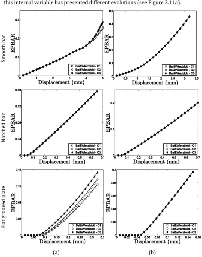
This chapter describes a simple and robust algorithm for numerical integration of a new model for metal plasticity and fracture. The constitutive model was proposed by Bai & Wierzbicki (2007) and critically includes both the pressure effect, through the stress triaxiality, and the effect of the third invariant of the deviatoric stress tensor, through the Lode angle, in the constitutive description of the material. These effects are directly introduced on the hardening rule of the material, which is typically only a function of the equivalent plastic strain. This approach is in contrast with the classical theory of metal plasticity, the so-called J2
theory, which assumes that both hydrostatic pressure and third invariant of the deviatoric stress tensor have a negligible effect on the material strain hardening and the flow stress. The model proposed by Bai and Wierzbicki was selected from the models available in literature for a detailed study and an implicit solution for numerical integration of Bai & Wierzbicki’s model is developed and implemented in an implicit quasi-static finite element environment. The algorithm is based on the operator split methodology, which to determine the stress update procedure, employs a fully implicit elastic predictor and plastic corrector (return mapping) step with general non-linear (piece-wise linear) isotropic hardening and the computation of the consistent tangent matrix (Simo et al., 1985 and 1987). Then, to illustrate the accuracy and stability of the integration algorithm in practical situations (Ortiz & Popov, 1985), iso-error maps are built for specific cases. At the end, the robustness of the numerical integration algorithm is demonstrated by a large group of numerical simulations where the numerical results are compared with experimental results for classical specimens as: a cylindrical smooth bar and a cylindrical notched bar modelled as two dimensional problems together with a flat grooved plate specimen simulated in three-dimensions.
32
3.1 INTRODUCTION
The theory based on the second invariant of the deviatoric stress tensor, , more widely known through von Mises’s model is one of the most used formulations to describe the behavior of metals, during the elasto-plastic regime. The von Mises’s model assumes that the effect of hydrostatic stress is negligible on the evolution of the plastic flow for ductile materials. The hydrostatic stress is a parameter responsible for controlling the size of the yield surface (Bardet, 1990; Bai, 2008). Furthermore, in the von Mises’s formulation, the effect of the third invariant of the deviatoric stress tensor, normally denoted by , is also ignored. The third invariant is a parameter used in the definition of the Lode angle or Azimuth angle, which is responsible for the shape of the yield surface (Bardet, 1990; Bai, 2008). Over the last five years, the importance of both hydrostatic stress and Lode angle, in the description of the behavior of ductile materials, has been clearly recognized and detail studies were conducted by several authors (Bai et al., 2007; Bai, 2008; Driemeier et al., 2010; Mirone et al., 2010; Gao et al., 2011). Many researchers have done extensive experimental studies as Richmond & Spitzing (1980 and 1984), who were the first researchers to study the effects of pressure on yielding of aluminum alloys. Latter, Bardet (1990), proposed a methodology to describe the Lode angle dependence for some constitutive models, and Wilson (2002), which conducted studies on notched 2024-T351 aluminum bars in tensile test and verified the importance of these effects. Brunig et al. (1999) proposed a constitutive model with three invariants that could be applied in metal plasticity and fracture. According to Mirone et al. (2010), the phenomenon of ductile failure is influenced by the relation with the variables from the stress–strain characterization and the failure prediction is better described by plastic strain, stress triaxiality and Lode angle parameters. An experimental program to study the influence of the stress tensor invariants in ductile failure was presented by Driemeier et al. (2010). This methodology can be seen as an efficient tool to investigate the effects of the stress intensity, stress triaxiality and Lode angle. Recently, Gao et al. (2011) have proposed an elasto-plastic model, which is a function of the hydrostatic stress as well as the second and third invariants of the stress deviator. These authors have carried out tests in specimens with a high level of stress triaxiality showing the dependence of the plastic flow rule on both stress
33
triaxiality and Lode angle. By examining these contributions, it is posible to conclude that ductile fracture is a local phenomenon and the stress and strain states over the expected fracture onset must be determined with accuracy. The fracture initiation is often preceded by large plastic deformation and there are considerable stress and strain gradients around the point of fracture. In this case, the theory is not accurate enough to capture the physical effects and more refined plasticity models have to be developed to be used in a large range of loading conditions.
3.2 PRELIMINARIES
Several factors have been systematically analyzed in the study of ductile fracture, nevertheless, there are three factors which have gained increased interest: the hydrostatic stress ( , stress triaxiality ( ), and the Lode angle expressed by Equations (3.1-3.3) respectively (Brunig et al., 2008; Bai & Wierzbicki, 2008; Zadpoor et al., 2009; Tvergaard, 2008; Nahshon et al., 2008).
(3.1) (3.2) { √ [ ( ) ]} (3.3)
where √ ⁄ is the von Mises equivalent stress, is the deviatoric stress tensor and , and are the components of the deviatoric stress tensor in the principal plane. The Lode angle can also be written as a function of the so-called normalized third invariant of the deviatoric stress tensor as:
(3.4)
where represents the normalized third invariant, that can be mathematically determined by a ratio between the third invariant and the von Mises equivalent stress: