R. Hosseini-Ara
[email protected] Isfahan University of Technology Department of Mechanical Engineering 84156-83111 Isfahan, Iran
H. R. Mirdamadi
[email protected] Isfahan University of Technology Department of Mechanical Engineering 84156-83111 Isfahan, Iran
H. Khademyzadeh
[email protected] Isfahan University of Technology Department of Mechanical Engineering 84156-83111 Isfahan, Iran
R. Mostolizadeh
[email protected] Isfahan University of Technology Department of Mechanical Engineering 84156-83111 Isfahan, Iran
Stability Analysis of Carbon
Nanotubes Based on a Novel Beam
Model and Its Comparison with
Sanders Shell Model and Molecular
Dynamics Simulations
We study the effects of small-scale parameter on the buckling loads and strains of nanobeams, based on nonlocal Timoshenko beam model. However, the lack of higher-order boundary conditions leads to inconsistencies in critical buckling loads. In this paper, we apply a novel approach based on nonlocal Timoshenko kinematics, strain gradient approach and variational methods for deriving all classical and higher-order boundary conditions as well as governing equations. Therefore, closed-form and exact critical buckling loads of nanobeams with various end conditions are investigated. Moreover, the dependence of buckling loads on the small-scale parameter as well as shear deformation coefficient is studied using these new boundary conditions. Then, numerical results from this new beam model are presented for carbon nanotubes (CNTs). They illustrate a more accurate buckling response as compared to the previous works. Furthermore, the critical strains are compared with results obtained from molecular dynamic simulations as well as Sanders shell theory and are found to be in good agreement. Results show that unlike the other beam theories, this model can capture correctly the small-scale effects on buckling strains of short CNTs for the shell-type buckling. Moreover, the value of nonlocal constant is calculated for CNTs using molecular dynamic simulation results.
Keywords: stability, nonlocal elasticity, carbon nanotubes, molecular dynamics
Introduction1
Structural elements like beams in nano-length scale are commonly used in nanotechnology devices such as NEMS. For devices of this size, the lengths are in the order of interatomic distances, so the nonlocal and small-scale effects can be significant. Generally, classic continuum theories are found to be inadequate because of their scale-free constitutive equations. In fact, these classic theories cannot capture the size effects. On the other hand, computational methods like Molecular Dynamics (MD) are not suitable for large-scale nano-structures because of their restricted capacities. Size-dependent continuum theories have thus received increasing attention in modeling nano-scale structures and devices. Among these, the theory of nonlocal continuum mechanics introduced by Eringen (1972; 1976; 1983 and 2002) and Eringen and Edelen (1972) has been widely used in nanomechanics for the small-scale effects. The characteristics of such theories are taking the internal length-scale and inter-atomic forces into consideration.
Nonlocal continuum mechanics has been applied in the areas of lattice dispersion of phonon waves, fracture and damage mechanics, wave propagation in nano composites, dislocation mechanics and surface tension in fluids, etc. (Eringen, 1983).
In particular, one property that has been extensively studied is the buckling of carbon nanotubes (CNTs), under axial compression (Yakobson et al., 1996; Peddieson et al., 2003; Wang et al., 2006; Sudak, 2003; Reddy and Pang, 2008; Reddy, 2007; Wang et al., 2010; Kumar et al., 2008; Feliciano et al., 2011; Zhang et al., 2004; Silvestre et al., 2011; Ma et al., 2008; Wang et al., 2010). Recently, some researchers investigated the free vibration and wave propagation of CNTs using nonlocal beam theories (Lu et al., 2006; Wang, 2005; Wang, C.M. et al., 2007; Wang, Q. and Wang, C.M., 2007; Yang et al., 2010; and Chang et al., 2002).
Paper received 18 September 2011. Paper accepted 21 November 2011 Technical Editor: Lavinia Borges
As mentioned before, the buckling equation of nanobeams modeled by nonlocal Timoshenko beam theory is a sixth-order differential equation and requires six boundary conditions including four classic (local) and two non-classic (higher-order) boundary conditions (Reddy and Pang, 2008). Researchers usually solve this equation without considering higher-order boundary conditions by neglecting the sixth-order term of the differential equation, because the higher-order boundary conditions are not determined clearly (Reddy and Pang, 2008). This approximation leads to inaccurate critical buckling loads.
This paper presents a novel method to derive the governing equations and all the classic and higher-order boundary conditions based on nonlocal continuum theory, strain gradient elasticity and variational method, simultaneously. Moreover, the exact and closed-form solutions of the critical buckling loads for nanobeams with various end conditions are investigated. The presented model includes the small-scale parameter and can simply degenerate into the other beam theories such as nonlocal Euler-Bernoulli, classical Timoshenko and classical Euler-Bernoulli beam models by ignoring either shear deformation parameter or nonlocal parameter or both of them, respectively.
Nonlocal Timoshenko Beam Theory
The nonlocal elasticity model was first presented by Eringen (1983). According to this model, the stress at a reference point in the body is dependent not only on the strain state at that point, but also on the strain state at all of the points throughout the body. The constitutive equation of the nonlocal elasticity can be written as follows (Eringen, 1983):
( )
(
1 2 2)
,0a ij Cijkl kl
e ∇ σ = ε
− (1)
where Cijkl is the elastic module tensor of the classical isotropic elasticity; and σijand εkl are the stress and strain tensors, respectively.
In addition, e is a nondimensional material constant, determined by 0
experiments, and a is an internal characteristic length (e.g., a lattice parameter, granular distance). Therefore, e0a is a constant parameter
showing the small-scale effect in nano-structures.
The assumed displacement field of the Timoshenko beam kinematics is
(
, , ,) ( )
,( )
, ,1x y zt uxt z xt
u = + φ
(
, , ,)
0,2x yzt =
u
(
, , ,) ( )
, ,3x y zt wxt
u =
(2)
where φ denotes the rotation of the cross section at point x about y-axis. The remaining nonzero axial and transverse shear strains are given by
,
x z x u
xx ∂
∂ + ∂ ∂
= φ
ε
.
2ε φ
γ +
∂ ∂ = ≡
x w
xz
(3)
The rotation of the cross section and the transverse shear strain are illustrated in Fig. 1 for a Timoshenko beam element as below:
Figure 1. Deformation components of a Timoshenko beam element.
Using Eq. (1), the nonlocal stress tensor components are
( )
2 ,2 2
0 xx
xx
xx E
x a
e σ ε
σ =
∂ ∂
−
( )
2 .2 2
0 γ
σ
σ KG
x a
e xz S
xz ∂ =
∂ −
(4)
The nonlocal stress resultants of axial force, shear, and bending moment are derived from the above equations, respectively:
( )
2 ,2 2 0
x u EA x N a e
N NL
NL ∂
∂ = ∂ ∂
− (5)
( )
2 ,2 2
0 KGAγ
x Q a e
Q NL S
NL ∂ =
∂
− (6)
( )
2 ,2 2 0
x EI x M a e
M NL
NL ∂
∂ = ∂ ∂
− φ (7)
where E, G, A and I are the Young's modulus, shear modulus, cross-sectional area of beam and area moment of inertia of beam cross section, respectively. Additionally, K denotes the shear correction S
factor, defined by
.
∫
=
A xz S dA
K
Q σ (8)
This factor corrects the assumption of constant shear strain on the cross section of beam in Timoshenko model, depending on the material and geometry of the cross section.
Strain Gradient Approach
Solving Eq. (4), the nonlocal axial and shear stresses as a function of displacement field can be determined as follows:
( )
,( ) ( )
,( ) ( ) ( )
, 4, ... , 44 0 2 2 2
0
+ ∂ ∂ + ∂ ∂ + =
x z x a e x
z x a e z x E z
x ε ε ε
σ (9a)
( )
( ) ( )
( ) ( ) ( )
4 ... .4 4 0 2 2 2
0
+ +
+ =
dx x d a e dx
x d a e x G K
x S
γ γ
γ
τ (9b)
Assuming ( 0 )2<<1
L a e
, where L is the length of the beam, and
neglecting the higher powers of the nonlocal parameter,
( )
2 0ae , the
solution could be simplified to
( )
,( ) ( )
,( )
2, ,2 2
0
∂ ∂ + =
x z x a e z x E z
x ε ε
σ (10a)
( )
( ) ( )
( )
2 .2 2
0
+ =
dx x d a e x G K
x S
γ γ
τ (10b)
In fact, Eqs. (10a) and (10b) can be thought of as constituting a strain gradient form of the nonlocal beam model (Peddieson et al., 2003). Considering strain gradient approach, for a Timoshenko beam subjected to an external compressive and conservative force field,
0
( ) ( )
( )
( )
( )
. 2 1 ) ( 2 2 ) ( , 2 2 , 0 2 0 0 0 0 2 2 0 2 2 2 0 2∫
∫
∫
∫
∫
− − + − + ∂ ∂ − = Π L L L V S S V dx dx dw N dx x w p dx dx du N dv dx x d G K a e x G K dv x z x E a e z x E γ γ ε ε (11)Thus, the second term is added to the original equation for capturing the shear deformation effects in Timoshenko beam theory. Furthermore, Chang et al. (2002) proved the original form of this equation for strain gradient theory without higher-order stress. They used characteristic size coefficient ( 2 6
d ) instead of nonlocal parameter and derived the potential energy density using integration by parts. The last three terms of Eq. (11) are also the work done by the axial load, lateral load and von Karman effect, respectively.
Substituting Eq. (3) into Eq. (11) and integrating over the cross-sectional area, the following expression is obtained for Π:
( )
( )
. 2 1 2 1 2 1 0 2 0 0 0 0 0 2 2 2 2 2 2 2 2 2 2 0 0 2 2 2∫
∫
∫
∫
∫
− − + + + + − + + + = Π L L L L S L S dx dx dw N dx x w p dx dx du N dx dx d dx w d GA K dx d EI dx u d EA a e dx dx dw GA K dx d EI dx du EA φ φ φ φ (12)Governing Equations and Boundary Conditions
The classical axial force, NCL, acting on the beam cross-section is defined as
.
dx du EA
NCL= (13)
Using the above expression for NCLand ignoring the laterally
distributed loads, p , for buckling analysis, the variation of Eq. (12) with respect to u
( )
x and equating to zero can be written as( )
( )
0.0 0 2 2 2 2 2
0 =
+ − =
Π
∫
dxdx u d N dx u d dx u d EA a e dx u d dx du EA L u δ δ δ δ (14)
Integrating by parts, we obtain the governing equation and boundary conditions in the x direction as
(
N +N0)
=0,dx d
NL (15)
(
+ 0)
0=0,= =
L x x NL N u
N δ (16)
( )
0.0 2
0 =
− = = L x x CL dx du dx dN a
e δ (17)
Performing the variation with respect to w
( )
x for Eq. (12) and equating to zero gives( )
( )
. 0 0 0 0 2 2 2 2 2 0 0∫
∫
∫
= − + − + = Π L L S L S w dx dx w d dx dw N dx dx w d dx d dx w d GA K a e dx dx w d dx dw GA K δ δ φ δ φ δ (18)Integrating by parts, we obtain the governing equation and boundary conditions for w as
2 2 0 dx w d N dx dQNL =
, (19)
, 0 0
0 =
− L NL w dx dw N
Q δ (20)
( )
0.0 2 2 2 0 = + − L S dx w d dx d dx w d GA K a
e φ δ (21)
In the same way, applying the variational operator to φ
( )
x for Eq. (12) and equating to zero, we obtain( )
( )
( )
0.0 2 2 2 0 0 0 2 2 2 2 2 0
∫
∫
∫
= + − + + − = Π L S L S L dx dx d dx d dx w d GA K a e dx dx dw GA K dx dx d dx d EI a e dx d dx d EI δφ φ δφ φ δφ φ δφ φ δφ (22)Using integration by parts, the governing equation is given by
, NL NL Q dx dM = (23)
and the following boundary conditions are derived:
( )
0,0 2 2 2 0 = + − L S NL dx d dx w d GA K a e
M φ δφ (24)
( )
0.0 2 2 2
0 =
− L dx d dx d EI a
e φ δφ (25)
By substituting the nonlocal shear force and bending moment defined in Eqs. (6) and (7) into the governing Eqs. (19) and (23), and omitting the similar terms from both sides of the equations, we obtain
( )
2,2 0 4 4 0 2 0 2 2 dx w d N dx w d N a e dx d dx w d GA
KS + =
+ φ (26a)
. 2 2 + = φ φ dx dw GA K dx d
EI S (26b)
( )
. 1 2 2 4 4 0 2 0 2 2 0 dx w d dx w d N a e dx w d N GA K dx d S − − = φ (27)By differentiating Eq. (26b) and inserting Eq. (27) in Eq. (26b), the transverse equilibrium equation in terms of lateral displacement for an axially loaded beam using a nonlocal strain gradient theory is obtained as
( )
( )
0,2 2 4 4 2 0 0 6 6 2
0 + =
− − + dx w d dx w d a e GA K EI N EI dx w d GA K a e EI S S (28)
where N is an external axial compressive load. This equation is 0
similar to that obtained by Reddy and Pang (2008) for buckling of the nonlocal Timoshenko beam using Hamilton's Principle.
In addition, for solving the above equation six boundary conditions are required (three for each end), but eight boundary conditions appear in Eqs. (20)-(21) and (24)-(25). It means that there is one additional boundary condition for each end. So, the main objective is to select three independent boundary conditions which can satisfy all four boundary conditions for each end. In the next part, the boundary conditions for various beam supports are obtained.
The nondimensional form of Eq. (28) using length of the beam,
L , as a nondimensionalizing parameter can be rewritten as
( )
1 2 0,2 4 4 2 2 6 6
4 + =
− Ω − + Ω dx w d dx w d r L dx w d L µ π µ (29)
where Ω and µ are the nondimensional forms of shear deformation and nonlocal parameters, respectively, and r is the ratio of the critical buckling loads as follows:
, 2 GAL K EI S = Ω , 2 0 = L a e
µ L ,
cr NL cr N N
r= (30)
where NL
cr
N is obtained from solving Eq. (28) and L cr
N is that given by classic Euler columns for simply supported end conditions.
We may simply switch to nonlocal Euler-Bernoulli beam model by ignoring the shear deformation terms. Also, the local Timoshenko beam model is obtained by letting the nonlocal parameter to be zero and by setting the shear deformation and nonlocal parameters to zero, the local Euler-Bernoulli beam model appears.
Buckling Solutions
Here we consider analytical solutions for nonlocal Timoshenko beams under a constant axial compressive load, using the buckling equation obtained in Eq. (28) for different end conditions. This sixth order equation exhibits different solutions which depend on the ratio
r, and the nonlocal and shear deformation parameters µ and Ω. The discriminant of the characteristic equation corresponding to the differential Eq. (28) is defined as follows:
( )
( )
. 4 1 4 2 2 4 2 0 2 2 0 0 Ω × − − Ω − = − − − = ∆ µ µ π r L GA K a e EI a e GA K EI N EI S S (31)If ∆>0, one of the solutions is
( )
( )
( )
cos( )
, sin cos sin ) ( 6 5 4 3 2 1 Qx c Qx c Px c Px c x c c x w + + + + + = (32)where c1,c2,...,c6 are constants of integration and determined by
six boundary conditions. P and Q are given by
( )
( )
2 1 2 0 2 0 02
∆ − − − = GA K a e EI a e GA K EI N EI P S S ,
( )
( )
. 2 2 1 2 0 2 0 0 ∆ + − − = GA K a e EI a e GA K EI N EI Q S S (33)If ∆<0, the other solution is defined as
( )
( )
( )
sin( )
, cos sin cos ) ( 6 5 4 3 2 1 Sx e c Sx e c Sx e c Sx e c x c c x w Rx Rx Rx Rx − − + + + + + = (34)where R and S are
( )
( )
( )
, 2 2 1 4 1 2 0 0 2 0 2 0 − + + = GA K EI a e N EI a e GA K EI a e EI GA K R S S S (35a)( )
( )
( )
. 2 2 1 4 1 2 0 0 2 0 2 0 − + − = GA K EI a e N EI a e GA K EI a e EI GA K S S S S (35b)The first solution in Eq. (32) is found to be valid depending on the sign of ∆. Therefore, the second solution is not used in this research and is only stated for completeness.
Simply supported beams
Considering the classic continuum mechanics for simply supported boundary conditions, the deflection and bending moment are zero at each end. We note that the essential boundary conditions are the same for the local and nonlocal boundary conditions. However, the natural boundary conditions should be transformed to the nonlocal form, in order that they can be used in higher-order theories. To this end, we use the classic boundary conditions as well as the newly derived boundary conditions in Eqs. (20)-(21) and (24)-(25) for deriving the following boundary conditions in order to satisfy all four boundary conditions:
, 0 =
, 0 2 2
= dx
w d
( )
4 0. 40 2
0 =
dx w d N a e
Inserting Eq. (36) into Eq. (32), we obtain a system of six homogeneous algebraic equations. In order to have a nontrivial solution, we should enforce the determinant of the coefficient matrix for the system of equations to be zero.
For simply supported conditions, the critical buckling load is obtained as
. ) ( )
(
2 0 4 2 0 2
2 4
2 2
GA K
a e EI a
e GA K
EI L L
EI L N
S S
Critical
π π
π
+
+ +
=
(37)
Manipulating the above equation using the dimensionless parameters µ and Ω, the critical buckling load becomes
. ) ( ) ( 1
1 4 2
2 2
Ω × + Ω + + =
µ π µ π π
L EI
NCritical (38)
This result is exactly the same as that obtained by Reddy (2007) using Fourier series and shows the perfect compatibility to the presented method. Reddy (2007) introduced the equation (38) as an exact solution for buckling of only simply supported beams. In his method, the series expansions of the generalized displacements are defined in order to satisfy the boundary conditions. However, it is not easy to define these series expansions of the generalized displacements for other boundary conditions such as clamped, cantilever or propped cantilever beams, but in the case of simply supported beams, it can verify Eq. (38) and new boundary conditions.
In addition, this result is similar to that obtained by Reddy and Pang (2008) using Hamilton's principle, except for an additional term which is the product of µ and Ω. This is due to neglecting the sixth-order term in solving the differential equation in the work of Reddy and Pang (2008). This equation is presented as follows:
. ) (
1 2
2
2
Ω + + =
µ π
π
L EI NT
Critical (39)
Moreover, this result could transform into the nonlocal Euler-Bernoulli forΩ=0, classical Timoshenko beam for µ =0 and
classical Euler-Bernoulli beam by letting Ω=µ=0.
Clamped beams
Regarding the classic continuum mechanics for clamped boundary conditions, the deflection and rotation of the cross-section are zero at each boundary. Thus, we use these classical as well as the newly derived boundary conditions in Eqs. (20)-(21) and (24)-(25) to derive the following boundary conditions. In this way we satisfy all four boundary conditions.
, 0 =
w
, 0
= dx
dw (40)
( )
(
)
3 0.3
0 5
5
0 2
0 + − =
dx w d N GA K dx
w d N a
e S
Substituting these boundary conditions in Eq. (32) and setting the determinant of the coefficient matrix to be zero, the critical buckling load is derived as
( )
16( )
. 44
2 0 4 2 0 2
2 4
2 2
GA K
a e EI a
e GA K
EI L L
EI L N
S S
Critical
π π
π
+
+ +
=
(41)
The critical buckling load using the dimensionless parameters µ and Ω is
. ) ( 16 ) ( 4 1
1
2
4 2
2 2
Ω × +
Ω + +
=
µ π µ
π π
L EI NCritical
(42)
Again, this equation may be transformed into either the nonlocal Euler-Bernoulli theory, for the shear parameter set to zero, ; the classical Timoshenko beam theory, for the nonlocal parameter set to zero, µ=0; or classical Euler-Bernoulli beam theory, for both the
shear and the nonlocal parameters set to zero, Ω=µ=0.
Cantilever beams
The boundary conditions for the fixed end of a cantilever beam at x=0 are derived in Eq. (40) for clamped beams. However, the
boundary conditions for the free end of a cantilever beam at x=L
are obtained based on the newly derived boundary conditions in Eqs. (20)-(21) and (24)-(25). Considering the classic boundary conditions, the shear force and bending moment are zero at the free end. Thus, we use these classic boundary conditions as well as the newly derived boundary conditions in Eqs. (20)-(21) and (24)-(25) to derive the following boundary conditions:
, 0 2 2
= dx
w d
, 0 4 4
= dx
w d
( )
( )
0.3 3 2 0 0
5 5 2
0 + =
− − +
dx dw dx
w d a e GA K
EI N EI dx
w d GA K
a e EI
S S
(43)
Again, these boundary conditions satisfy Eqs. (20)-(21) and (24)-(25). Applying these boundary conditions and solving the transcendental equation corresponding to the determinant of the coefficient matrix, the critical buckling load is obtained
( )
( )
.4 4
2 0 4 2 0 2
2 4
2 2
GA K
a e EI a
e GA K
EI L L
EI L N
S S
Critical
π π
π
+
+ +
=
(44)
. ) ( 16
1 ) ( 4 1 1
1
5 . 0
4 2
2 2
Ω × +
Ω + +
=
µ π µ
π π
L EI NCritical
(45)
This result is similar to that obtained by Reddy and Pang (2008) for cantilever beams, except an additional term which is the product of µ and Ω. Again, this is due to neglecting the sixth-order term in solving the differential equation in their work. This equation is presented as below:
. ) (
4 2
2
2
Ω + + =
µ π
π
L EI NT
Critical (46)
Thus, in the case of cantilever beams, it can verify Eq. (45) and new boundary conditions in Eqs. (40) and (43) derived from variational approach.
Propped cantilever beams
The boundary conditions for propped cantilever beams are the combination of clamped and simply supported boundary conditions, derived before. Assuming the fixed end at x=0 and hinged end at
L
x= , we have Eqs. (40) and (36) for the fixed and hinged boundary conditions, respectively.
Solving the determinant equation of the coefficient matrix, results the critical buckling load as below:
. ) ( 184 . 4 ) ( 045
. 2
045 . 2
2 0 4 2
0 2
2 4
2 2
GA K
a e EI a
e GA K
EI L L
EI L N
S S
Critical
π π
π
+
+ +
=
(47)
Hence, the critical buckling load using the dimensionless parameters µ and Ω is
. ) ( 515 . 407 ) ( 187 . 20 1
1
43 . 1
2 2
Ω × +
Ω + +
=
µ µ
π
L EI NCritical
(48)
Generalizing, the closed-form and exact solution of critical buckling load for nonlocal Timoshenko beam with various end conditions is investigated as
( )
( )
,) ( ) ( 1
1
4 2
2 2
Ω × +
Ω + +
=
µ π µ
π π
k k
k L EI NCritical
(49)
where k is a constant depending on different boundary conditions and defined as k=1 for simply supported, k=2 for clamped, k=0.5 for cantilever and k=1.43 for propped cantilever beams considered for the fundamental mode of buckling load. This is a remarkable result which can relate the nonlocal solutions with the small-scale effects to the classical solutions of the beams.
Defining the equivalent values for length, nonlocal and shear deformation parameters as follows:
,
k L
leq= ,
2 0
=
eq eq
l a e
µ 2 ,
eq S eq
GAl K
EI =
Ω (50)
where l is an equivalent length, defined for buckling of columns eq
with different boundary conditions.
.
2 2
eq classic cr
l EI
N =π (51)
Simplifying Eq. (49) by using equivalent values in Eq. (50), we obtain
. ) (
) (
1
1
4 2
2 2
Ω × + Ω + + =
eq eq eq
eq eq
Critical
l EI N
µ π µ
π π
(52)
In addition, this result can simply degenerate into the nonlocal Euler-Bernoulli beam theory for Ωeq=0, classical Timoshenko beam theory for µeq=0 and classical Euler-Bernoulli beam model by letting Ωeq=µeq=0.
Numerical Results
Comparison of critical buckling loads for beam theories
In this section, we consider numerical solutions for CNTs modeled as nanobeams with circular cross sections. The numerical results are presented in the form of graphs and tables for different types of end conditions, using the following effective properties of carbon nanotubes (Reddy and Pang, 2008):
. 877 . 0 ), ( 5 . 1
) ( 049 . 0 64 , ) ( 785 . 0 4
) ( 1 , ) ( 420 , ) ( 1000
4 4
2 2
= =
= = =
=
= =
=
S K nm a
nm d
I nm d
A
nm d GPa G
GPa E
π π
(53)
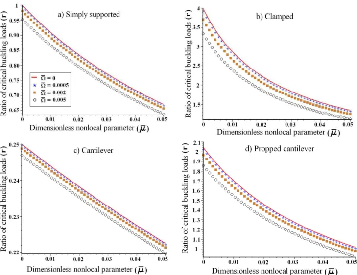
Plots of the critical buckling loads for nonlocal Timoshenko beam for different values of shear deformation and nonlocal parameters are presented in Fig. 2.
As illustrated in Fig. 2, the solid lines for Ω=0 denote Euler-Bernoulli beam which are the upper bound solutions. By increasing the shear deformation parameter, Ω, the critical buckling loads decrease. The effect of shear deformation is quantified for different boundary conditions. This effect is negligible for L /d ratios more than 20 (or Ω less than 0.0005), but significant by increasing the
Ω, for L /d ratios less than 20.
Moreover, the intersections of the curves and the y-axes (i.e., 0
=
µ ) are the ratios of the local critical buckling loads. Specifically, for Ω=0, these values are the same as the local Euler-Bernoulli beam solutions.
Figure 2. Plots of the ratios of the buckling loads for different values of µand Ω and various boundary conditions.
Table 1. Comparison of the ratio of the critical buckling loads for simply supported beams with respect to nonlocal Euler-Bernoulli, Timoshenko and exact Timoshenko solutions.
00170
.
0
=
Ω
Ω
=
0
.
00075
Ω
=
0
.
00042
µ
NEBT NTBT Exact rµ
NEBT NTBT Exact rµ
NEBT NTBT Exact r0 1 0.9835 0.9835 0 1 0.9927 0.9927 0 1 0.9959 0.9959
0.0025 0.9759 0.9602 0.9598 0.0011 0.9893 0.9820 0.9819 0.0006 0.9939 0.9900 0.9900 0.01 0.9102 0.8965 0.8952 0.0044 0.9584 0.9516 0.9513 0.0025 0.9759 0.9720 0.9719 0.0225 0.8183 0.8072 0.8048 0.01 0.9102 0.9041 0.9035 0.0056 0.9474 0.9437 0.9434 0.04 0.7170 0.7085 0.7051 0.0178 0.8506 0.8452 0.8443 0.01 0.9102 0.9067 0.9064
Table 2. Comparison of the ratio of the critical buckling loads for clamped beams with respect to nonlocal Euler-Bernoulli, Timoshenko and exact Timoshenko solutions.
00170
.
0
=
Ω
Ω
=
0
.
00075
Ω
=
0
.
00042
µ
NEBT NTBT Exact rµ
NEBT NTBT Exact rµ
NEBT NTBT Exact r0 4 3.7491 3.7491 0 4 3.8845 3.8845 0 4 3.9342 3.9342
Table 3. Comparison of the ratio of the critical buckling loads for cantilever beams with respect to nonlocal Euler-Bernoulli, Timoshenko and exact Timoshenko solutions.
00170
.
0
=
Ω
Ω
=
0
.
00075
Ω
=
0
.
00042
µ
NEBT NTBT Exact rµ
NEBT NTBT Exact rµ
NEBT NTBT Exact r0 0.25 0.2490 0.2490 0 0.25 0.2495 0.2495 0 0.25 0.2497 0.2497
0.0025 0.2485 0.2474 0.2474 0.0011 0.2489 0.2489 0.2489 0.0006 0.2496 0.2494 0.2494 0.01 0.2440 0.2430 0.2430 0.0044 0.2469 0.2469 0.2469 0.0025 0.2485 0.2482 0.2482 0.0225 0.2368 0.2359 0.2359 0.01 0.2435 0.2436 0.2435 0.0056 0.2466 0.2463 0.2463 0.04 0.2275 0.2267 0.2266 0.0178 0.2390 0.2390 0.2390 0.01 0.2440 0.2438 0.2438
Table 4. Comparison of the ratio of the critical buckling loads for propped cantilever beams with respect to nonlocal Euler-Bernoulli, Timoshenko and exact Timoshenko solutions.
00170
.
0
=
Ω
Ω
=
0
.
00075
Ω
=
0
.
00042
µ
NEBT NTBT Exact rµ
NEBT NTBT Exact rµ
NEBT NTBT Exact r0 2.0449 1.9773 1.9773 0 2.0449 2.0143 2.0143 0 2.0449 2.0276 2.0276
0.0025 1.9467 1.8853 1.8823 0.0011 2.0005 1.9712 1.9705 0.0006 2.0193 2.0023 2.0022 0.01 1.7014 1.6543 1.6451 0.0044 1.8781 1.8522 1.8500 0.0025 1.9467 1.9309 1.9302 0.0225 1.4062 1.3739 1.3597 0.01 1.7014 1.6801 1.6760 0.0056 1.8362 1.8222 1.8207 0.04 1.1313 1.1103 1.0939 0.0178 1.5043 1.4877 1.4818 0.01 1.7015 1.6894 1.6870
As it may be observed from Tables 1-4, the first row of each table indicates the local form (i.e., µ=0) and in this state the solution of the nonlocal Timoshenko beam without higher-order boundary conditions and exact nonlocal Timoshenko beam are the same. This is due to ignoring the nonlocal parameter that leads to ignoring the higher-order boundary conditions.
In general, the shear deformation and nonlocal parameters have the effect of reducing the buckling loads. This effect is the most significant for clamped beams (up to 7%) and the least significant for cantilever beams (about 1%).
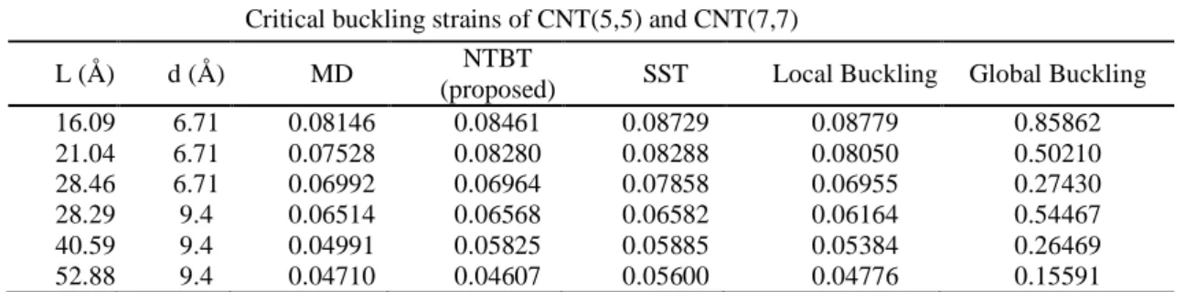
Validation of critical buckling strains
In this subsection, the numerical results for critical buckling strains obtained from this continuum mechanics theory are compared with those obtained from MD simulations and Sanders shell theory (Silvestre et al., 2011). Since the MD simulations referenced herein consider the CNTs with fixed ends, we also consider the NTBT model with fully clamped boundary conditions. In addition, CNT(5,5) is analyzed with a diameterd=6.71Å and
CNT(7,7) with a diameterd=9.40Å, for different lengths. Both
nanotubes are modeled using a thickness h=0.66Å, Young’s
modulus E=5.5TPa and Poisson’s ratio ν=0.19 (Yakobson et al., 1996). The results from MD simulations, nonlocal Timoshenko beam and Sanders shell models are compared in Table 5.
It is seen that the critical buckling strains are in good agreement as compared with the results obtained from MD simulations as well as Sanders shell theory. Moreover, the results show that unlike the other beam theories, this model could capture correctly the length-dependent buckling strains of short CNTs for the mode of shell-type buckling. In fact, the available beam models are unable to show the correct trend in critical axial buckling strains of short CNTs, while the proposed nonlocal beam model shows much better agreement with the molecular dynamics simulation results.
Finally, based on the MD simulation results, the value of nonlocal constant is determined for CNTs based on an averaging process. The best match between MD simulations and nonlocal formulations is achieved for a nonlocal constant value of e0a=0.3
for CNT(5,5) and e0a=0.53 for CNT(7,7), with good accuracy (the
error is less than 10%).
Table 5. Comparison between critical buckling strains of CNT(5,5) and CNT(7,7) obtained from MD simulations, Sanders shell theory (SST) (Silvestre et al., 2011), and proposed nonlocal Timoshenko beam theory (NTBT).
Critical buckling strains of CNT(5,5) and CNT(7,7)
L (Å) d (Å) MD NTBT
(proposed) SST Local Buckling Global Buckling
16.09 6.71 0.08146 0.08461 0.08729 0.08779 0.85862
21.04 6.71 0.07528 0.08280 0.08288 0.08050 0.50210
28.46 6.71 0.06992 0.06964 0.07858 0.06955 0.27430
28.29 9.4 0.06514 0.06568 0.06582 0.06164 0.54467
40.59 9.4 0.04991 0.05825 0.05885 0.05384 0.26469
Conclusions
Nonlocal Timoshenko beam model was developed and buckling behavior of CNTs was analyzed using a mixed approach based on the strain gradient theory and variational method of total potential energy. This approach provides the governing equations and variationally consistent sets of boundary conditions for various end supports.
In addition, the exact and closed-form eigenvalues of the nonlocal critical buckling loads for nanobeams with various end conditions were investigated, which are more complete and accurate compared with those available in the literature. These solutions could simply be reduced to the nonlocal Euler-Bernoulli, classical Timoshenko and classical Euler-Bernoulli beam models by ignoring the nondimensional shear deformation parameter Ω, nonlocal parameter µ or both of them, respectively.
Moreover, the small-scale effects and shear deformation parameter are specifically highlighted for this model using higher-order boundary conditions. In this case, it is clearly observed that the critical buckling loads obtained from Eq. (52) for all different boundary conditions are always smaller than those predicted by the classical model. In fact, the nonlocal parameter µ and shear
deformation parameter Ω have the effect of reducing the buckling load. This effect is the most significant for clamped beams (up to 7%) and the least significant for cantilever beams (about 1%).
References
Chang, C.S., Askes, H., Sluys, L.J., 2002, “Higher-order strain/higher-order stress gradient models derived from a discrete microstructure, with application to fracture”, Engineering Fracture Mechanics, 69, pp. 1907-1924.
Eringen, A.C., 1972, “Nonlocal polar elastic continua”, Int. J. Eng. Sci., 10, pp. 1-16.
Eringen, A.C., 1976, “Continuum Physics Volume IV: Polar and Nonlocal Field Theories”, Academic Press, New York.
Eringen, A.C., 1983, “On differential equations of nonlocal elasticity and solutions of screw dislocation and surface waves”, J. Appl. Phys., 54, pp. 4703-4710.
Eringen, A.C. and Edelen, D.G.B., 1972, “On nonlocal elasticity”, Int. J. Eng. Sci., 10, pp. 233-248.
Feliciano, J., Tang, C., Zhang, Y., Chen, C., 2011, “Aspect ratio dependent buckling mode transition in single-walled carbon nanotubes under compression”, J. Appl. Phys., 109, 084323.
Kumar, D., Heinrich, C., Waas, A.M., 2008, “Buckling analysis of carbon nanotubes modeled using nonlocal continuum theories”, J. Appl. Phys., 103, 073521.
Lu, P., Lee, H.P., Lu, C., Zhang, P.Q., 2006, “Dynamic properties of flexural beams using a nonlocal elasticity model”, J. Appl. Phys., 99, 073510.
Ma, H.M., Gao, X-L., Reddy, J.N., 2008, “A Microstructure-Dependent Timoshenko Beam Model Based on a Modified Couple Stress Theory”, Journal of the Mechanics and Physics of Solids, 56, 3379-3391.
Peddieson, J., Buchanan, G.R., McNitt R.P., 2003, “Application of nonlocal continuum models to nanotechnology”, Int. J. Eng. Sci., 41, pp. 305-312.
Reddy, J.N., 2007, “Nonlocal theories for bending, buckling and vibration of beams”, Int. J. Eng. Sci., 45, pp. 288-307.
Reddy, J.N., Pang, S.D., 2008, “Nonlocal continuum theories of beams for the analysis of carbon nanotubes”, J. Appl. Phys., 103, 023511.
Silvestre, N., Wang, C.M., Zhang, Y.Y., Xiang, Y., 2011, “Sanders shell model for buckling of single-walled carbon nanotubes with small aspect ratio”, Composite Structures, 93, pp. 1683-1691.
Sudak, L.J., 2003, “Column buckling of multi-walled carbon nanotubes using nonlocal continuum mechanics”, J. Appl. Phys., 94, pp. 7281-7287.
Wang, B., Zhao, J., Zhao, S., 2010, “A micro-scale Timoshenko beam model based on strain gradient elasticity theory”, Eur. J. Mech. A/Solids, 29, pp. 591-599.
Wang, C.M., Zhang, Y.Y., He, X.Q., 2007, “Vibration of nonlocal Timoshenko beams”, Nanotechnology, 18, 105401.
Wang, C.M., Zhang, Y.Y., Xiang, Y., Reddy, J.N., 2010, “Recent Studies on Buckling of Carbon Nanotubes”, Appl. Mech. Rev., 63, 030804.
Wang, Q., 2005, “Wave propagation in carbon nanotubes via nonlocal continuum mechanics”, J. Appl. Phys., 98, 124301.
Wang, Q., Varadan, V.K., Quek, S.T., 2006, “Small scale effect on elastic buckling of carbon nanotubes with nonlocal continuum models”, Phys. Lett. A, 357, pp. 130-135.
Wang, Q., Wang, C.M., 2007, “The constitutive relation and small scale parameter of nonlocal continuum mechanics for modeling carbon nanotubes”, Nanotechnology, 18, 075702.
Yakobson, B.I., Brabec, C.J., Bernholc, J., 1996, “Nanomechanics of carbon tubes: instabilities beyond linear response”, Phys. Rev. Lett., 76, pp. 2511-2514.
Yang, J., Ke, L.L., Kitipornchai, S., 2010, “Nonlinear free vibration of single-walled carbon nanotubes using nonlocal Timoshenko beam theory”, Physica E, 42, pp. 1727-1735.