Acoustic communications in water pipes

(1)

University of Aveiro

2017

Department of

Electronics, Telecommunications and Informatics

Daniel

da Silva Almeida

Comunicações acústicas em tubos com água

(2)

(3)

Daniel

da Silva Almeida

Comunicações acústicas em tubos com água

Acoustic communications in water pipes

Dissertação apresentada à Universidade de Aveiro para cumprimento dos requisitos necessários à obtenção do grau de Mestre em Engenharia Eletrónica e Telecomunicações, realizada sob a orientação científica dos Doutores João Nuno Matos e José Neto Vieira, Professores Associado e Auxiliar, respetivamente, do Departamento de Eletrónica, Telecomunicações e Informática da Universidade de Aveiro

University of Aveiro

2017

Department of

(4)

(5)

(6)

(7)

o júri / the jury

presidente / president _{Professor Doutor João Manuel de Oliveira e Silva Rodrigues} Professor Auxiliar da Universidade de Aveiro

vogais / examiners committee _{Doutora Catarina Maria Brito de Noronha Santiago} Profissional de Engenharia, nível 2, Bosch Termotecnologia, S.A. (arguente principal)

Professor Doutor José Manuel Neto Vieira

(8)

(9)

acknowledgements _{I want to thank the teacher José Neto Vieira for being always}

available to help and orient me during this project. His close presence, the long hours of conversation, the encouragement and constant stimulus were essential for the completion of this thesis. I want to thank the teacher João Nuno Matos for his help and regular supervision especially in the first half of this project. I want to thank my family, especially my parents and brothers, for always being there for me.

I want to thank Eduardo Miranda, Pedro Machado and João D’Ascensão for the help provided in the setups of the last experiment.

As this thesis represents the last stage of a long academic

journey, I would like to express my sincere gratitude to the friends I made along it.

(10)

(11)

palavras-chave Comunicações digitais, transdutores piezoelétricos, tubos com água.

resumo _{Este documento apresenta uma abordagem experimental da}

implementação de comunicação digital entre dois pontos usando tubos com água como infraestrutura e transdutores piezoelétricos de baixo custo. Este documento explica o procedimento, passo a passo, dos conceitos necessários para a análise do tubo como canal de comunicação de dados e a implementação e avaliação de um sistema de comunicação digital usando modulações ASK e BPSK. Os transdutores foram fabricados para operar no ar com uma frequência central de 40 kHz, mas o meio água alterou a sua frequência operacional central para aproximadamente 63.7 kHz e 69 kHz e é mostrado que, sem a presença de bolhas, é possível estabelecer uma comunicação confiável e, portanto, transmitir dados. O objetivo deste documento é também introduzir, ao leitor não especializado, conceitos de correlação, canal como filtro e modulações ASK e BPSK, o que permitirá compreender as discussões relacionadas com este estudo.

Para realizar os testes, foi montado um sistema com computador portátil, placa de som, amplificador, dois transdutores e vários tipos de montagem de tubos.

Após a introdução do Capítulo 1, o Capítulo 2 apresenta o estado da arte dos sistemas de comunicação em tubos. O Capítulo 3 expõe o software e o hardware utilizados. O Capítulo 4

caracteriza o tubo como um canal, onde são obtidas as suas respostas ao impulso e em frequência e cada componente da montagem do tubo é analisada quanto à atenuação que causa. O Capítulo 5 apresenta as modulações ASK e BPSK seguidas pelas experiências de transmissão de dados usando as mesmas. O Capítulo 6 oferece as conclusões finais e dicas para trabalho futuro. Finalmente, o Capítulo 7 fornece as referências que apoiam este documento.

(12)

(13)

keywords _{Digital communications, piezoelectric transducers, water pipes.}

abstract _{This document presents an experimental approach of}

implementing a digital communication between two points using water pipes as infrastructure and low-cost piezoelectric based transducers. It explains the procedure, step by step, of the concepts required for the analysis of the pipe as a data

communication channel and the implementation and evaluation of a digital communication system using ASK and BPSK

modulations. The transducers were manufactured to operate in air with a centre frequency of 40 kHz, but the water medium changed its operating centre frequency to approximately 63.7 kHz and 69 kHz and it is shown that without the presence of bubbles, it is possible to establish a reliable communication and therefore, transmit data. The objective of this thesis is also to introduce a non-expert reader into concepts of correlation, channel as a filter and ASK and BPSK modulations, which will allow to understand the discussions related to this study.

To perform the tests, a system was assembled with laptop, sound board, amplifier, two transducers and various type of pipe setups. Following the introduction of Chapter 1, Chapter 2 presents the state of the art of in-pipe communications systems. Chapter 3 exposes the software and hardware used. Chapter 4

characterizes the pipe as a channel, where is it obtained its impulse and frequency responses and each component of the pipe channel is analysed regarding the attenuation that causes. Chapter 5 introduces ASK and BPSK modulations followed by the data transmission experiments using the same. Chapter 6 offers the final conclusions and future work tips. Finally, Chapter 7 provides the references that support this document.

(14)

(15)

List of Figures

Figure 1 - The most common applications of underwater communications. [3] ... 4

Figure 2 - Pipeline as a waveguide. ... 5

Figure 3 - MCUSD14A40S09RS transducer. [15] ... 12

Figure 4 - Technical terms of the transducers. [15] ... 12

Figure 5 - Setup of the experiment with the transducers facing each other. ... 14

Figure 6 - Speakers Properties: Sample rate and bit depth. ... 16

Figure 7 - Microphone Properties: Sample rate and bit depth. ... 16

Figure 8 - Speakers Properties: Levels. ... 17

Figure 9 - Microphone Properties: Levels. ... 17

Figure 10 - Front view of the sound card. ... 18

Figure 11 - Back view of the sound card. ... 19

Figure 12 - Quad-Capture Control Panel. ... 20

Figure 13 - Amplifier frequency response (first signal is the input of the amplifier and the second is the output). ... 22

Figure 14 - Envelope of the normalized calibration. ... 23

Figure 15 - Calibrated input signal. ... 23

Figure 16 - Spectrogram of the calibrated input signal. ... 24

Figure 17 – Calibrated signal at the input of the amplifier ([1, 85] kHz). ... 24

Figure 18 - Signal at the output of the amplifier ([1, 85] kHz). ... 25

Figure 19 - Balanced connections. [17] ... 25

Figure 20 - Noise cancellation. [18] ... 26

Figure 21 - The XLR connector, seen from its front. ... 26

Figure 22 - Transducer, seen from side. ... 27

Figure 23 - Output connection with the 6.3 mm stereo jack, seen from side. ... 27

Figure 24 - Cables assembly complete scheme. ... 28

Figure 25 - Appearance of the connection cable with stereo jack. ... 29

Figure 26 - Appearance of the connection cable with XLR connector. ... 29

Figure 27 - Ends of the pipe capped by a rubber material. ... 30

Figure 28 - Side view of the mechanical coupling between the pipe and the transducer. ... 31

(18)

Figure 30 – Nyquist-Shannon sampling theorem. [22] ... 33

Figure 31 - Cross-correlation between y(n) and x(n) ... 35

Figure 32 - Cross-correlation between y(n) and x(n), with channel noise r(n) ... 36

Figure 33 - Setup used for the experiments. ... 40

Figure 34 - Setup with the pipe, the sound card and the receiver and transmitter transducers. ... 41

Figure 35 - Experiment with the fixed receiver transducer (brown) and the transmitter transducer (grey) at a given distance. ... 41

Figure 36 – Received signal of the transmission between the fixed receiver transducer and the transmitter transducer at 20 centimetres. ... 42

Figure 37 - Gain as a function of distance in the experiment with the fixed receiver transducer... 43

Figure 38 - Experiment with the fixed transmitter transducer (grey) and the receiving transducer (brown) at a given distance. ... 44

Figure 39 - Gain as a function of distance in the experiment with the fixed transmitter transducer... 44

Figure 40 - Setup of the experiment with fixed transducers at the ends of the pipe. ... 46

Figure 41 – Transmitter transducer fixed to a pipe connector. ... 47

Figure 42 – Receiver transducer fixed to a pipe connector. ... 47

Figure 43 - Transmitter transducer. ... 48

Figure 44 - Receiver transducer... 49

Figure 45 - Setup with the 1-meter pipe with a male tee connector in the middle. ... 50

Figure 46 - Setup with the 0.8 meters pipe ... 51

Figure 47 - Setup with the 1-meter pipe ... 51

Figure 48 – Voltage output for different setups. ... 52

Figure 49 - Chirp spectrogram x(n). ... 54

Figure 50 - Normalized autocorrelation of the input signal x(n). ... 55

Figure 51 - Filter impulse response. ... 56

Figure 52 – Filter frequency response. ... 57

Figure 53 - Signal at the receiver transducer. ... 58

Figure 54 - Impulse response for the pipe with 0.8 meters of length. ... 59

(19)

Figure 56 - Setup with the 4.5 meters pipe (receiver side). ... 61

Figure 57 - Setup with the 4.5 meters pipe (transmitter side). ... 62

Figure 58 - Setup with the 4.5 meters pipe. ... 63

Figure 59 - Impulse response for the pipe with 4.5 meters of length filled with air. ... 64

Figure 60 - Frequency response for the pipe with 4.5 meters of length filled with air. ... 64

Figure 61 - Impulse response for the pipe with 4.5 meters of length filled with water... 65

Figure 62 - Frequency response for the pipe with 4.5 meters of length filled with water... 66

Figure 63 - Impulse response for the pipe with 4 meters of length filled with water... 67

Figure 64 - Frequency response for the pipe with 4 meters of length filled with water... 67

Figure 67 - Impulse response for the pipe with 3 meters of length filled with water... 70

Figure 68 - Frequency response for the pipe with 3 meters of length filled with water... 70

Figure 71 - Impulse response for the pipe with 4.5 meters of length filled with water with a male tee connector at the receiver side. ... 72

Figure 72 - Frequency response for the pipe with 4.5 meters of length filled with water with a male tee connector at the receiver side. ... 73

Figure 73 - Impulse response for the pipe with 1 meter of length filled with water with a male tee connector in the middle. ... 74

Figure 74 - Frequency response for the pipe with 1 meter of length filled with water with a male tee connector in the middle. ... 74

Figure 75 - Setup with the 0.8 meters pipe filled with water with a male knee connector. 75 Figure 76 - Impulse response for the pipe with 0.8 meters of length filled with water with a male knee connector at the receiver side. ... 76

Figure 77 - Frequency response for the pipe with 0.8 meters of length filled with water with a male knee connector at the receiver side. ... 76

Figure 78 - Voltage attenuation for a given length of the pipe (Straight setup). ... 79

Figure 79 – Frequency response in the band [60, 75] kHz for the longer length pipes experiments. ... 80 Figure 80 - Impulse response of the raised-cosine filter with various roll-off factors. [26] 84

(20)

Figure 81 - Frequency response of the raised-cosine filter with various roll-off factors. [26]

... 84

Figure 82 - Consecutive raised-cosine impulses, demonstrating zero-ISI property. [27] ... 85

Figure 83 – The modulated carrier for a given sequence of 1’s and 0’s. ... 86

Figure 84 – Modulating signal with bandwidth B. ... 87

Figure 85 – Modulated carrier with bandwidth 2 B. ... 87

Figure 86 - Power spectral density of the ASK signal. ... 88

Figure 87 - The PSK signal. ... 88

Figure 88 - PSK demodulator. ... 90

Figure 89 - Block diagram of a circuit that obtains a coherent local carrier. ... 91

Figure 90 - PSK receiver with carrier extractor. ... 91

Figure 91 - ASK implementation diagram. ... 94

Figure 92 – BPSK implementation diagram. ... 95

Figure 93 – Number of errors per threshold % for the data transmission using the 4.5 meters pipe filled with air and ASK modulation... 96

(21)

List of Tables

Table 1 - Characteristics of Electromagnetic, Optical and Acoustic waves underwater. ... 3

Table 2 - Constituents of a sensor system. ... 6

Table 3 - Specific Acoustic Impedance of certain materials. [10], [11] ... 8

Table 4 – Some characteristics of some experiments done in water pipes... 9

Table 5 - Voltage output, gain and central frequency at a given distance in the experiment shown in Figure 5. ... 14

Table 6 - Headphones vs sound card peak-to-peak output voltage for a given amplitude in Audacity. ... 21

Table 7 - Voltage attenuation as function of a given distance (short length pipes). ... 78

Table 8 - Voltage attenuation as function of a given distance (longer length pipes). ... 79

Table 9 - Voltage attenuation for the Branch setup as function of a given distance. ... 81

Table 10 - Voltage attenuation for the Bent setup as function of a given distance. ... 82

Table 11 - Data transmission using the 4.5 meters pipe filled with air and ASK modulation. ... 96

Table 12 - Data transmission using the 4.5 meters pipe filled with air and BPSK modulation. ... 97

Table 13 - Data transmission using the 4.5 meters pipe filled with water and ASK modulation (𝑓𝑐= 69000 Hz). ... 97

Table 14 - Data transmission using the 4.5 meters pipe filled with water and BPSK modulation (𝑓𝑐= 69000 Hz). ... 98

Table 15 - Data transmission using the 4 meters pipe filled with water and ASK modulation (𝑓𝑐= 64500 Hz). ... 99

Table 16 - Data transmission using the 4 meters pipe filled with water and BPSK modulation (𝑓𝑐= 64500 Hz). ... 99

Table 17 - Data transmission using the 3.5 meters pipe filled with water and ASK modulation (𝑓𝑐= 63700 Hz). ... 100

Table 18 - Data transmission using the 3.5 meters pipe filled with water and BPSK modulation (𝑓𝑐= 63700 Hz). ... 100

Table 19 - Data transmission using the 3 meters pipe filled with water and ASK modulation (𝑓𝑐= 69500 Hz). ... 101

(22)

Table 20 - Data transmission using the 3 meters pipe filled with water and BPSK modulation (𝑓𝑐= 69500 Hz). ... 102 Table 21 - Data transmission using the 2.5 meters pipe filled with water and ASK modulation (𝑓𝑐= 63700 Hz). ... 103 Table 22 - Data transmission using the 2.5 meters pipe filled with water and BPSK modulation (𝑓𝑐= 63700 Hz). ... 103 Table 23 - Data transmission using the 4.5 meters pipe filled with water, tee connector at the receiver side and ASK modulation (𝑓𝑐= 69000 Hz). ... 104 Table 24 - Data transmission using the 4.5 meters pipe filled with water, tee connector at the receiver side and BPSK modulation (𝑓𝑐= 69000 Hz). ... 105 Table 25 - Data transmission using the 1-meter pipe filled with water, tee connector in the middle and ASK modulation (𝑓𝑐= 63700 Hz). ... 106 Table 26 - Data transmission using the 1-meter pipe filled with water, tee connector in the middle and BPSK modulation (𝑓𝑐= 63700 Hz). ... 107 Table 27 - Data transmission using the 0.8 meters pipe filled with water, knee connector at the receiver side and ASK modulation (𝑓𝑐= 69500 Hz). ... 108 Table 28 - Data transmission using the 0.8 meters pipe filled with water, knee connector at the receiver side and BPSK modulation (𝑓𝑐= 69500 Hz). ... 109

(23)

Abbreviations and Symbols

°C Degree Celsius

A/D Analog-to-digital converter CPU Central processing unit D/A Digital-to-analog converter dB Decibel F0 Initial frequency F1 Final frequency Fs Sampling frequency Hz Hertz k kilo kg kilogram m metre M Mega Pa Pascal

rayl Unit of acoustic impedance R Correlation

Rn Normalized correlation Rx Receiver

s second Tx Transmitter

USB Universal Serial Bus Vp-p peak-to-peak Voltage z Specific acoustic impedance

(24)

(25)

1. Introduction

In today’s society, water distribution networks are a vital infrastructure. Numerous devices such as sensors, consumption meters, control elements, among others, are installed within the distribution network to control and ensure the correct supply. There should be periodical reviews and monitorization to assure the proper functioning of these devices and distribution networks. However, physical access can be difficult because some places are relatively inaccessible. That is why the use of devices that allow remote control with a minimum maintenance would create great solutions with benefits in terms of remote access and cost.

Despite the extensive research in open sea underwater applications, there has not been much research on acoustic communication systems in water pipes. In the pipes, acoustic waves have been also widely studied, not for communication purposes but for leakage detection.

The use of devices that allow the performance of supervision tasks remotely, reduction of maintenance and costs, would guarantee a huge progress in terms of obtaining information of the distribution network.

The communication system described in this document is based on digital communication using ultrasounds and low-cost commercial hardware, inside a PEX pipe that represents the waveguide channel. There, the propagation of the acoustic wave will suffer several distorting phenomena, such as multipath propagation and reflections, which alter its shape, amplitude, frequency and phase characteristics, therefore parameters such as pipe material and fittings, length, bends and branches greatly affect the transmission properties, which will all be subject of analysis.

The motivation for researching in this area came from the possible utility of information transmission in this medium and the endless solutions that this kind of

(26)

technology can offer to the water distribution networks frequently used in houses and factories, where the possibility of ultrasound transmission would lead to improvements and to innovative solutions in applications such as central energy consumption monitoring units, control of the valves or flows, among others.

This project aims to develop a low cost acoustic communications system that uses the hydraulic water distribution system for communication between devices. This solution can be used for short distance communication between hydraulic systems such as water heaters, valves and other types of sensors.

The main objectives are to study the water pipe as a data communication channel and study the data transmission using some basic modulations.

(27)

2. Communications using water pipes

Over the past decades underwater communication has been considered a very active research area since it facilitates the needs of many military or, more recently, commercial operations. Underwater communication is required for applications to provide communication with submarines, communication between divers, command of autonomous underwater vehicles, animal tracking, sea bed exploration, pollution monitoring, remote control of off-shore equipment, data collection from deep sea sensors, among others. These applications of underwater communication rely mostly on the transmission of acoustic waves. Optical and electromagnetic waves have also been studied but results conclude they are not very efficient. Electromagnetic waves have very high rates of absorption (limits the practical bit rate that can be achieved) in this environment which complicates the propagation of long distances in water. Also, its attenuation by scattering is high and increases with frequency and per kilometer. An additional problem is the requirement of large antennas and high-power transmitters for electromagnetic waves communication. On the contrary, optical waves are not so affected by absorption but they are affected by scattering. [1]

Opposed to electromagnetic and optical waves, acoustic waves are less affected by absorption and scattering by water.

Waves Rates of absorption Attenuation by scattering

Electromagnetic High High

Optical Low High

Acoustic Low Low

(28)

The use of underwater acoustic waves was recognized long time ago as a way of communication and detection. Leonardo da Vinci wrote in 1490: "If you cause your ship to stop and place the head of a long tube in the water and place the outer extremity to your ear, you will hear ships at a great distance from you ". [2]

Figure 1 - The most common applications of underwater communications. [3]

Despite the extensive research in open sea underwater applications [4] [5], there has not been much research on acoustic communication systems in water pipes. Mainly, the studies purposes of acoustic waves in pipes are not about communications but for leakage detection. [6] [7]

The acoustic channels in the ocean are characterized with respect to the location of the transmitter and receiver as horizontal or vertical and as deep or shallow. Such standardization does not exist for in-pipe acoustic channels, since parameters such as pipe material, geometry, elbows, connections and valves, as well as the length of the ramifications highly affect the transmission properties.

Time variation of environmental variables, which is significant in the ocean, is minimal in the pipeline system. Waves, fish, ships, temperature and so on are constantly

(29)

changing the characteristics of the open sea acoustic channel, while for the in-pipe acoustic waveguide channel only daily or seasonal variations of temperature may slightly affect the system.

Figure 2 - Pipeline as a waveguide.

The power resources are limited inside the water pipe, and therefore it is necessary to implement an energy efficient communication system. Since water pipes are usually within the walls or below the floor, the wireless sensor nodes will not be accessible for battery replacement or maintenance, therefore the presence of a constant power supply is indispensable. A potential source of energy could be the flow of water inside the pipeline. In such case the power harvesting system would be composed of a small generator connected to a propeller driven by the water flow. However, the capacity of such a system is totally dependent to the flow velocity. The normal operation of the water pipe needs to be considered as well, limiting the size of the turbine used.

Water pipes supply potable water to communities, consequently, health considerations are far more stringent in such systems than in the ocean. Any device installed inside a water pipe must be rigorously tested for compatibility with the environment and cannot change the properties of the water.

A sensor system is composed by four interconnected modules: CPU (A/D and/or D/A conversion of the information, signal processing and storage of sensor inputs), power batteries (needs to be power efficient and minimize the energy required), communication (unit responsible for the transmission and reception of data from neighboring sensor modules) and sensors (piezoelectric for our purposes). [1]

(30)

Constituents of a sensor system:

CPU Power batteries Communication

Sensors

Table 2 - Constituents of a sensor system.

Piezoelectricity is the ability to produce electricity through the compression on certain materials. In this work, piezoelectric transducers will be used, and the mechanical pressure will be performed by the ultrasound waves.

Multipath propagation of the transmitted wave is the most important signal distortion phenomenon in underwater acoustic communications. Most solutions are based on the idea of transmitting a narrow beam to achieve minimum interaction with the boundaries and create a single path of wave propagation. For this reason, many implementations have introduced long transmitting arrays that are capable of beamforming the transmitted signal and directing it to a specific target. [8] The beamwidth is defined as the width of the main lobe in degrees, and it is measured between the points where the power has dropped 3dB. Beam steering is achieved by use of proper phase or time delays between signals driven by the transducer array. Each type of transducers has its specific characteristics such as construction, size and shape to generate beams of specific pattern and beamwidth. For instance, spherical transducers provide an omnidirectional pattern, while others can generate elliptical, toroidal, or conical patterns. The amount of applications is numerous.

The successful implementation of an underwater communication also depends on the hardware, which includes hydrophones (for receiving sound), projectors (for transmitting sound) or transducers (for both receiving and transmitting), along with preamplifier or power amplifier units to drive the receiver or transmitter respectively. These devices can be set alone or laid in an array configuration. To complete the communications system, it is necessary a software with the communication protocol, an analog to digital converter for the

(31)

receiver, a digital to analog converter for the transmitter and undoubtedly a power supply. From now on, the devices capable of transmitting and/or receiving acoustic signals, will be referred as transducers.

To select an appropriate transducer, there are many parameters that need to be defined, such as resonant frequency, efficient bandwidth, beam pattern, beam width, directivity, transmitting power, receiving sensitivity. Furthermore, depending on the type of application, parameters such as size, weight, operational depth, lifetime, material, type of power supply, among others, may become of critical importance.

Because of the limitations of the bandwidth of the underwater acoustic channel, the efficiency of the bandwidth range is perhaps the most important characteristic of an underwater acoustic transducer. The frequency content of the transmitted signal affects the bit rate and the quality of the received signal. Consequently, a transducer with a good transmitting and/or receiving frequency band is required for the robustness of the acoustic signal. Outside of this band, any transmitted or recorded signal has its characteristics significantly affected.

The challenges of developing water pipe communication include the characterization of the water pipe acoustic channel for narrowband and wide band scenarios, noise and interference characterization and physical layer communication techniques for the unique water pipe channel.

Acoustic impedance will be discussed in the next Chapters, therefore it is useful to know this set of variables and equations for acoustic impedance (Z) and specific acoustic impedance (z): [9]

• p = density = 1000 kg/m3_(water)

• v = speed propagation (water 20 °C) = 1480 m/s • S is the surface.

• z is expressed in (Pa s/m) or rayl. • Z is expressed in (Pa s/m3_{) or (rayl/m}2_).

z = 𝑝 𝑣

(1) Z = 𝑝 𝑣_𝑆

(32)

In water 20ºC, z = 1.48 M Pa s/m.

The Table 3 shows values of density, ultrasound speed and specific acoustic impedance for various materials at a temperature of 20ºC.

Material _{Density (}𝑘𝑔 𝑚3) Ultrasound waves speed (m/s) z (M rayl) Aluminium 2700 6300 17.01 Iron 7870 5900 46.43 Cast iron 7207 4600 33.15 Polyethylene 900 1900 1.71 Air 1,3 330 0.00043 Water 1000 1480 1.48 Copper 8940 4700 42.02

Table 3 - Specific Acoustic Impedance of certain materials. [10], [11]

Regarding experiments in water pipes, there is some examples. Here there is the purpose of the researches and some of its characteristics. The paper [12] studies the communication in water pipes. The paper [13] studies the acoustic channel. The paper [14] studies the wide modeling of the acoustic water pipe channel. The paper [1] performs experiments in air using PVC pipes but then converts the results by a relation between the speed of the ultrasound waves in air and in water.

(33)

Paper/thesis Bit rate (Hz) Distance (m) Modulation Carrier frequency (kHz) Type of pipe [12] 31; 63 6 BPSK, QPSK 2.5 Iron [13] - 1; 2 - 30 Copper [14] 25.6 k 6.3 OFDM BPSK 32.5 PVC [1] 1 k; 4 k; 7 k from 10 to 30 FSK, ASK, QAM 9.1 PVC

(34)

(35)

3. Software and hardware used

3.1 Software

3.1.1 Audacity

It is an audio editor and recorder software. It is a good alternative to the signal generator and oscilloscope set because it allows the signals analysis and its recording. In this document, it will be used to generate sine tones and sine chirps. Its ability to plot spectrum and spectrogram graphic is very important for the analysis of the signals recorded.

3.1.2 MATLAB

It is a multi-paradigm numerical computing environment. In this document, MATLAB is used for all the simulations, signal and data processing and plotting. The main toolboxes used are the Signal Processing Toolbox and Communications System Toolbox. All the functions and coding used in the experiments presented in this document were created by the author, except for the cases where it is said that a certain MATLAB function was used.

3.2 Hardware

3.2.1 Transducers

One of the first tasks is to choose an appropriate type of transducer to allow the acoustic communication in water. Some of the most important characteristics when

(36)

searching for this type of transducers are their centre frequency, type of construction, sensitivity, beam pattern, allowable input voltage, size, consumption and its cost. It is necessary that the transducers have their centre frequency in the acoustic range, a type of construction that allows the operation in the water medium, high sensitivity, narrow beam pattern, high allowable input voltage, small size, low consumption and they need to be cheap. A research was done in some of the distributors that usually provide materials for the Institute of Telecommunications of Aveiro and due to its low price (5.06 €), one of the first transducers found was the MCUSD14A40S09RS transducer from Farnell with the following technical terms. [15]

Figure 3 - MCUSD14A40S09RS transducer. [15]

(37)

In the datasheet provided, it was written the target applications of this transducer, quoting, “This specification covers the water proof type ultrasonic ceramic transducer which are used for ultrasonic ranging and parking sensor of automobile.” [15]

Analysing the important characteristics stated previously, it is possible to conclude that this transducer does not fulfil all the needs. Its construction is not meant for underwater, it is water proof, which means it can work in humid environments and handle rain, but it is not built to be constantly underwater, therefore it was not possible to know if the transducers would work underwater and if so, it is assured that the water would change the operating mode of the transducer. The centre frequency, sensitivity, allowable input voltage, size and using method fulfil the needs, but the beam pattern is too wide while it was required a narrow pattern to lower the reflexions inside the water pipe. Regarding consumption, it was only stated that it has low power consumption.

More research was done to find a better transducer but all it was found was very expensive transducers (more than two hundred euros) which get bigger the lower the frequency, therefore it would not fulfil the need of the size and hydrophones which are even more expensive (around one thousand euros or more) and even though its housing would fulfil the needs, it is too big in terms of length which would hinder the insertion of the hydrophone is a piping system. Therefore, considering the low price of the transducer shown previously, it was decided to order 4 of it and this transducer will be used for all the experiments shown in this document.

According to Table 3 in Chapter 2, the specific acoustic impedance, z, is 0,00043 M rayl for air and 1.48 M rayl for water, therefore it is expected that the water environment will cause huge attenuations because of the acoustic impedance mismatch between the water and the transducer that was manufactured to operate in air.

3.2.1.1 Testing the transducers

The first experiments were done without any pipe, wherein the transducers were facing each other at a given distance.

(38)

In Figure 5, at the right there is a signal generator connected to the transmitter transducer and at the left there is the receiver transducer connected to an oscilloscope.

Figure 5 - Setup of the experiment with the transducers facing each other.

The amplitude of the sine wave generated in the signal generator is 20 Vp-p. The input voltage is kept unchanged throughout the tests, which results are shown in the Table 5.

Distance (cm) 𝑉 𝑝−𝑝𝑜𝑢𝑡 (mV) Voltage Gain (dB) Central frequency (kHz)

2 102 -45.85 41.50

3.5 80 -47.96 41.55

8 72 -48.87 41.71

12.5 56.8 -50.93 41.25

(39)

The band of frequency that provides at least _√21 (-3 dB) of the maximum output voltage is approximately from 40 kHz to 42.5 kHz. In this experiment, there was not used any fixing support, so it is impossible to guarantee that the transducers are parallel to each other (face to face), but it was useful to verify some of the characteristics of the transducers. The transducer transmits all around itself due to the vibration of its housing. For the cases where the transducers were side by side or with their back facing each other, the transmission was very low. For the case where the transducers were facing each other, a better transmission was obtained, as it was expected.

3.2.2 Use of the headphones and microphone outputs

The first experiments with the transducers and the Audacity for signal generation and recording were performed with the use of the headphones and the microphone outputs of the laptop. For that, it is necessary to take in consideration the speakers and the microphone properties which can be found in the Sound settings in Windows Control Panel. It is necessary to guarantee that the sample rate selected in the Advanced tab is the same of the one selected when creating the input signal in Audacity.

(40)

Figure 6 - Speakers Properties: Sample rate and bit depth.

Figure 7 - Microphone Properties: Sample rate and bit depth.

It is important to adjust the microphone gain according to the magnitude of the received signal, otherwise the received signal might saturate and therefore its spectrogram

(41)

will not provide a good analysis of the received signal. The Microphone Boost can be selected from 0 to +30 dB.

Figure 8 - Speakers Properties: Levels.

(42)

3.2.3 Sound card Roland - QUAD-CAPTURE

It was considered that the use of the headphones and microphone outputs was not the best approach, so it was chosen to use the sound card shown in the Figure 10 because of its kit. Some of the characteristics of this sound card are two XLR/TRS inputs with premium mic preamps, headphone output, graphical control panel software which provides fast and intuitive control of the preamps (see Figure 12), low-noise wide-range power supply, low latency performance and 24-bit/192 kHz audio quality. These preamps deliver an accurate and neutral sound across the entire frequency spectrum, with no bias towards any particular frequency band. In addition, they also deliver lots of headroom. Increasing the headroom in mic preamps typically results in problems with the signal-to-noise ratio, however, with its power supply circuitry, the noise levels are minimized while providing a wider dynamic range. [16]

(43)

The receiver transducer connects to Input 1L (Sens 1L at 100%), the Input 2R is kept off, the potentiometer is on playback and the transmitter transducer connects to the output (output at 100%).

It is important to have the potentiometer on playback, otherwise there would be feedback whereas the sound card would be reproducing the input signal plus the output signal which would lead to errors in the analysis of the transmission.

Figure 11 - Back view of the sound card.

The USB connection is the power supply and the mean of communication with the laptop. The selects Ground lift, Phantom and Hi-Z are kept off. The sound card has the advantage of having a control panel to manage the specifications of the preamp, compressor and mixer (see Figure 12).

Throughout this document, the only specification that is subject to changes in the QUAD-CAPTURE Control Panel is the SENS (sensitivity), which is changed according to the amplitude of the sound card input signal (received signal of the transmission), from 0 to 54 dB. Since the equation for the sound card sensitivity was not available, to know the voltage amplitudes of the signals recorded, each sensitivity used in the experiments was

(44)

characterized in terms of its relation between input voltage amplitude and the amplitude recorded in Audacity, using a known signal provided by the signal generator.

Figure 12 - Quad-Capture Control Panel.

3.2.3.1 Output voltage of the headphones and the sound card

As stated previously, there is two ways of making the signal generated in Audacity arrive to the transmitter transducer: by connecting it to the headphones output of the laptop or by connecting it to the sound card which is connected to the laptop by USB. Thus, it is necessary to measure the both outputs for a given Audacity amplitude, which can be seen in the Table 6.

(45)

Amplitude of the signal generated in Audacity Output voltage of the headphones of the laptop (Vp-p) Output voltage of the sound card

(Vp-p) 1 4.08 7.00 0.9 3.7 6.64 0.8 3.26 5.84 0.7 2.9 5.00 0.6 2.46 4.32 0.5 2.06 3.58 0.4 1.66 2.88 0.3 1.28 2.16 0.2 0.85 1.44 0.1 0.44 0.73

Table 6 - Headphones vs sound card peak-to-peak output voltage for a given amplitude in Audacity.

3.2.4 Grundig V 304 amplifier

As shown in Table 6, the maximum output voltage the sound card can provide from a maximum Audacity amplitude signal is 7 Vp-p, which is not enough voltage for the experiments with pipes because the attenuation will be high, and the system would not use the high capability of the supported input voltage of the transducers. Therefore, it was necessary to use an amplifier to provide a higher voltage to the transmitter transducer.

To study the frequency response of the Grundig V 304 amplifier, a linear sine chirp with amplitude 1 (maximum amplitude in Audacity) and frequency band from 1 Hz to 96 kHz, half of the sampling frequency, was sent and its response was recorded. As it is possible

(46)

to observe in the Figure 13, the amplifier does not have a constant amplitude frequency response. Lower frequencies suffer a greater amplification than higher frequencies which leads to misinterpretations in the frequency response of the experiments with the pipes. To calibrate the amplifier frequency response, it is necessary to make adjusts to the input signal.

Figure 13 - Amplifier frequency response (first signal is the input of the amplifier and the second is the output).

In MATLAB, it was obtained the envelope of both signals. The envelope of the input signal (constant value equal to 1) was divided by the envelope of the output signal and then the amplitude was normalized so the maximum amplitude would be 1, as shown in Figure 14.

𝐶𝑎𝑙𝑖𝑏𝑟𝑎𝑡𝑖𝑜𝑛 = 𝐼𝑛𝑝𝑢𝑡_𝐸𝑛𝑣𝑒𝑙𝑜𝑝𝑒

𝑂𝑢𝑡𝑝𝑢𝑡_𝐸𝑛𝑣𝑒𝑙𝑜𝑝𝑒 (3)

𝑁𝑜𝑟𝑚𝑎𝑙𝑖𝑧𝑒𝑑 𝐶𝑎𝑙𝑖𝑏𝑟𝑎𝑡𝑖𝑜𝑛 = 𝐶𝑎𝑙𝑖𝑏𝑟𝑎𝑡𝑖𝑜𝑛

(47)

Figure 14 - Envelope of the normalized calibration.

The envelope of the normalized calibration was multiplied by a sine linear chirp with frequency band from 1 Hz to 96 kHz and the result is represented in the Figure 15.

(48)

The spectrogram in Figure 16 confirms the frequency linearity of the sine chirp and the frequency band.

Figure 16 - Spectrogram of the calibrated input signal.

Despite the calibration done was theoretically correct, the amplifier was not responding as expected for frequencies lower than approximately 1 kHz and higher than approximately 85 kHz, therefore it was chosen to restrict the band of analysis to [1, 85] kHz (see Figure 17).

(49)

Figure 18 - Signal at the output of the amplifier ([1, 85] kHz).

In the Figure 18, it is not important to note on the amplitude because that is a matter of the sensitivity used but what is important is that the output signal of the amplifier is constant and it will be used as the input signal at the transmitter transducer.

3.2.5 Cables assembly

The type of cables used are balanced cables. Balanced connections are intended to eliminate noise from the channel that the signals go through. A balanced system has 3 different wires: positive (hot), reverse positive (cold) and neutral (ground).

Figure 19 - Balanced connections. [17]

The emitting source sends the signal in two different wires, inverting the phase in one of them (cold). Any noise that affects the signals will be of equal polarity in both wires. The receiver unit inverts the phase of the cold signal causing the signal to return to its correct polarization, therefore by adding the hot signal and the inverted cold signal, the noise is

(50)

cancelled. In the Figure 20, it is shown how a glitch is cancelled in a balanced system, where at the end of the process there is the sent signal without noise and with twice the amplitude.

Figure 20 - Noise cancellation. [18]

End with XLR connector:

One conductor (hot) was welded to the XLR_Pin2, the other conductor (cold) to the XLR_Pin3 and the shielding to the ground (XLR_Pin1).

(51)

End with transducer:

The respective conductor of the XLR_Pin2 was welded to the Transducer_Pin1. It was confirmed that the transducer aluminium housing is short-circuited with the Transducer_Pin2, so the conductor corresponding to the "XLR_3-Cold" pin and the shielding corresponding to the "XLR_1-Ground" pin were welded to the Transducer _Pin2. The transducer and the connections were wrapped in aluminium foil, short-circuiting the aluminium housing to the shielding.

Figure 22 - Transducer, seen from side.

End with 6.3 mm stereo jack:

(52)

Figure 24 - Cables assembly complete scheme.

A study on magnetic field shielding properties concluded that the assembly of the Figure 24 provides 77 dB of magnetic noise attenuation, therefore it will be used for the experiments present in this document. [19]

Since the transducer housing is short-circuited with the Transducer_Pin2, there is a balanced connection only until the pins of the transducer. Yet, this change is expected to protect the communication from the power grid noise. Both transducers and shielding from the end containing a transducer were wrapped in aluminium foil to isolate the transducers of any type of noise, especially the receiver transducer, which receives voltages in the order of millivolts, therefore it is indispensable to use the insulator material.

The appearance of the cables after their assembly is shown in the Figure 25 and in the Figure 26.

(53)

Figure 25 - Appearance of the connection cable with stereo jack.

(54)

3.2.6 Pipe channel

The type of pipe used is PEX (polyethylene material [20]) and it has 20 mm of external diameter and 15.5 mm of internal diameter. Various pipe lengths will be studied along this document.

The first setups with the pipe will be designated as straight. However, the pipes are not totally straight as they were rolled up to be transported.

Figure 27 - Ends of the pipe capped by a rubber material.

The mechanical coupling between the transducer and the pipe is achieved through elastics which ensure that the transducer is in contact with the pipe. This solution has the defect of not being a rigid fixation, therefore the area of contact is not always the same, which means that the transducer sometimes is not at the ideal position, where the centre of the transducer would be in contact with the centre of the curvature of the pipe.

(55)

Figure 28 - Side view of the mechanical coupling between the pipe and the transducer.

Figure 29 - Top view of the mechanical coupling between the tube and the transducer.

The explanation of procedure of the cables and pipe assemblies show how the first setups were performed. If there will be any change in the cables or the type of setup, it will be indicated along with their experiments.

(56)

(57)

4. Characterization of the water pipe channel

4.1 Introduction

The Nyquist–Shannon sampling theorem is a fundamental bridge between continuous-time signals and discrete-continuous-time signals. To guarantee the perfect reconstruction, the sample-rate, Fs (samples/second), needs to be higher than twice the bandwidth B. Equivalently, for a given sample rate, the bandlimit B needs to be lower than half of Fs. If these conditions are not fulfilled, the signal reconstruction has imperfections known as aliasing, which is an effect that causes different signals to become indistinguishable (or aliases of one another) when sampled. [21]

(58)

The measurement of impulse responses is a common task in different areas (especially important in audio processing). In theory, any input signal with a high bandwidth can be used to measure the impulse response of a linear system.

The output signal can be expressed in terms of the impulse response by:

𝑦[𝑛] = ℎ[𝑛] ∗ 𝑥[𝑛] = ∑ ℎ[𝑘] ∙ 𝑥[𝑛 − 𝑘]

∞

𝑘=0

(5)

Assuming the impulse response only has N significant samples and L is the length of the input signal, the former equation can be rewritten in a matrix form as:

(6)

Then, the impulse response can be theoretically obtained as:

(7)

Where the matrix X-1* represents the pseudo-inverse of matrix X: (XT·X)-1·XT or

XT·(X·XT)-1.

However, in practice, very long input signals would be needed to attain high suppression of measurement noise, resulting in extremely large problems which may turn out to become computationally intractable. [23]

An attractive approach consists in using as input signal one which auto-correlation function is similar to a delta sequence, which is a discrete impulse signal:

                                          [ 1] ] 1 [ ] 0 [ ] 1 [ 0 0 0 ] 0 [ ] 1 [ 0 0 ] 0 [ ] 2 [ ] 1 [ ] 0 [ N h h h L x x x x L N y y y                                                     ] 2 [ ] 1 [ ] 0 [ ] 1 [ 0 0 0 ] 0 [ ] 1 [ 0 0 ] 0 [ ] 1 [ ] 1 [ ] 0 [ 1* L N y y y L x x x x N h h h         

(59)

𝑅_𝑥𝑥[𝜏] = 1

2 𝑁 + 1 ∑ 𝑥[𝑛 + 𝜏] ∙ 𝑥[𝑛] ≈ 𝛿[𝜏]

𝑁

𝑛=−𝑁

(8)

In this case, the impulse response of the system can be obtained by cross-correlating the output and the input signals:

Figure 31 - Cross-correlation between y(n) and x(n)

Assuming the length of the input signal is K and that the impulse response has only N significant samples, we have the following equations for the output signal, y, and for the cross-correlation: 𝑦[𝑛] = ∑ ℎ[𝑘] ∙ 𝑥[𝑛 − 𝑘] 𝐾+𝑁−1 𝑘=0 (9) 𝑅𝑦𝑥[𝜏] = 1 𝐾 ∑ 𝑦[𝑛 + 𝜏] ∙ 𝑥[𝑛] 𝐾−1 𝑛=0 (10)

Replacing y [n + τ] in the equation (10) results in:

𝑅𝑦𝑥[𝜏] = 1 𝐾 ∑ ∑ ℎ[𝑘] ∙ 𝑥[𝑛 + 𝜏 − 𝑘] ∙ 𝑥[𝑛] = ∑ ℎ[𝑘] 1 𝐾 ∑ 𝑥[𝑛 + 𝜏 − 𝑘] ∙ 𝑥[𝑛] 𝐾−1 𝑛=0 𝐾+𝑁−1 𝑘=0 𝐾+𝑁−1 𝑘=0 𝐾−1 𝑛=0 (11)

(60)

As mentioned previously, it is considered that the autocorrelation function of the input signal is similar to a discrete impulse signal:

1

𝐾 ∑ 𝑥[𝑛 + 𝜏 − 𝑘]𝑥[𝑛] ≈ {1 𝜏 = 𝑘0 𝜏 ≠ 𝑘

𝐾−1

𝑛=0

(12)

Which will result in the following approximation:

𝑅_𝑦𝑥[𝜏] ≈ ℎ[𝜏]

(13)

Using this indirect approach, a great immunity against noise is achieved. The energy of the input signal can be as large as desired, since it is just necessary to extend its duration. [23]

Figure 32 - Cross-correlation between y(n) and x(n), with channel noise r(n)

The equation (14) represents the diagram of the Figure 32.

𝑦[𝑛] = ∑ ℎ[𝑘]𝑥[𝑛 − 𝑘] + 𝑟[𝑛]

𝐾+𝑁−1

𝑘=0

(14)

As noise corrupting the output signal is uncorrelated with the input signal x, its contribution in the measurement of the impulse response is very small, as it is

(61)

𝑅_𝑦𝑥[𝜏] ≈ ℎ[𝜏] +1

𝐾 ∑ 𝑟[𝑛 + 𝜏]𝑥[𝑛] ≈ ℎ[𝜏]

𝐾−1

𝑛=0

(15)

Even though it was explained how cross-correlation can be used to obtain the impulse response of a system, it has not been introduced properly yet in this document.

First of all, an explanation about autocorrelation will be provided. The amplitude distribution of a sequence does not tell if successive sample values are related to one another. Nevertheless, it is possible to characterize the time domain structure of a sequence using the autocorrelation function, which is the average of the inner product of the sequence x[n] with a time shifted version of itself. Autocorrelation is a valuable measure of the statistical dependence among values of x[n] at different times (see equation (16) ), and summarises its time domain structure. [24]

𝑅𝑥𝑥[𝜏] = 1 2 𝑁 + 1 ∑ 𝑥[𝑛 + 𝜏]𝑥[𝑛] 𝑁 𝑛=−𝑁 (16)

When a sequence is autocorrelated, its autocorrelation sequence has a large central peak at τ = 0, with small non-zero values at both sides. At zero-time shift, the signals match perfectly, positive and negative values align with themselves resulting a large positive value, but at any other value of time shift, a given sample is just as likely to align with one of the opposite sign, so the average of the cross-product is approximately zero, therefore, there is no correlation between adjacent samples. The central value of an autocorrelation function is equal to the mean square value of the sequence, and is, therefore, a measure of its total power. The central value, 𝑅_𝑥𝑥(0) for x(n) or 𝑅_𝑦𝑦(0) for y(n), is always the maximum value. It can be equal for other values of time shift, but it can never be exceeded. [24]

The correlation between two signals measures the degree of similarity between those two signals. In digital communications, the received signal, y(n), is massively corrupted by the additive white Gaussian noise (AWGN) to the point where a visual analysis might not reveal the presence or absence of the transmitted signal. Cross-correlation provides means for extracting that important information from y(n).

(62)

𝑅_𝑥𝑦(𝜏) = ∑ 𝑥(𝑛)𝑦(𝑛 − 𝜏) 𝜏 = 0, ±1, ±2, … 𝑁 𝑛=−𝑁 (17) 𝑅𝑥𝑦(𝜏) = ∑ 𝑥(𝑛 + 𝜏)𝑦(𝑛) 𝜏 = 0, ±1, ±2, … 𝑁 𝑛=−𝑁 (18)

The index τ is the time shift or lag and the subscripts x and y on the cross-correlation sequence 𝑅_𝑥𝑦(𝜏) indicate the sequences being correlated. The order of the subscripts indicates de direction in which one sequences is shifted relatively to the other. To clarify, in the equation (17), the sequence x(n) is left unshifted and y(n) is shifted by τ units in time, to the right for positives values of τ and to the left for negative values of τ. Equivalently, in the equation (18), the sequence y(n) is left unshifted and x(n) is shifted by τ units in time, to the left for positive values of τ and to the right for negative values of τ. Clearly, both equations produce the same cross-correlation sequence. By swapping the subscripts x and y of the cross-correlation sequence, a folded version is obtained, where the folding is done with respect to τ = 0. Therefore, 𝑅𝑦𝑥(𝜏) provides the same information regarding the similarity

of x(n) to y(n). As they are folded versions of each other, the sign of τ where the correlation has the maximum value is positive for one case and negative for the other. Considering that x(n) is the transmitted signal and y(n) is the received signal, ignoring the AWGN and possible attenuations, y(n) is a delayed version of x(n), therefore the maximum value of correlation for 𝑅𝑥𝑦(𝜏) occurs for a negative value of τ and for a positive value of τ for 𝑅𝑦𝑥(𝜏).

[23]

It is important to note that cross-correlation is not the same of convolution. In the calculation of convolution, one of the sequences is folded, then shifted, then multiplied by the other sequence to form the product sequence for that shift and finally the values of the product sequence are added. Except for the folding operation, the calculation of the cross-correlation sequence involves the same operations.

(63)

In practice, it is often performed the normalizations of the autocorrelation and cross-correlation sequences to the amplitude range [-1, 1] because any value of cross-correlation can easily be misunderstood when there is not a reference value. Therefore, the normalized autocorrelation sequence, 𝑅𝑛𝑥𝑥(τ), is defined as:

𝑅𝑛_𝑥𝑥(τ) =_𝑅𝑅𝑥𝑥(τ)

𝑥𝑥(0)

(19)

Similarly, the normalized cross-correlation sequence, 𝑅𝑛_𝑥𝑦(τ), is defined as: 𝑅𝑛_𝑥𝑦(τ) = 𝑅𝑥𝑦(τ)

√𝑅𝑥𝑥(0) 𝑅𝑦𝑦(0)

(20)

Before going into the experiments, it is important to note some of the characteristics of the sound wave. The sound wave is a longitudinal wave. For this type of wave, the particles of the medium move in a direction parallel to the direction that the wave moves. It is also a mechanical wave because it requires a medium to transport their energy from one location to another. [25]

4.2 First experiments with pipes

As explained in the previous section, cross-correlation techniques are used to measure the degree of similarity between two signals. Since the same device (laptop) processes the transmitted and the received signals, a good implementation for the synchronization between those signals can be achieved using cross-correlation. The delay τ that causes the highest amplitude of 𝑅_𝑦𝑥(τ), in other words, that causes the best correlation between the two signals is considered to be the real delay of the whole transmission from the point where the signal is sent from the laptop to the point where it is received at the same device. Most of the delay is caused by the sound card latency and just a small part of the delay reflects the transmission time between the transducers through the water pipe. To explain the procedure, consider the transmitted signal to have N samples. The received signal has a greater number of samples,

(64)

considering the transmission has delay and the receiver records for a greater amount of time than the time that the transmitted signal last. From the received signal, it will be selected only the samples from τ+1 to τ+N, thus the latency and the final part of the received signal are removed, therefore the new received signal has the same number of samples of the transmitted signal, N, and it is the part of the received signal that has better correlation with the transmitted signal.

The latency does not have a fixed value, generally it is equal to a value from 80 to 100 ms. The reason of this variation is caused by the different processing times that the laptop, the sound card and the amplifier take.

The experiments described in this document follow the diagram setup of the Figure 33, except for the amplifier, which is used from section 4.2.3 onwards.

(65)

4.2.1 Experiments with the transducers in perpendicular with the tube

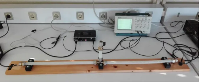
Figure 34 - Setup with the pipe, the sound card and the receiver and transmitter transducers.

The following test was performed with the receiver transducer attached to one end of the pipe, which was filled with water, and the transmitter transducer situated at a given distance. The input signal is a tone with carrier frequency of 40 kHz with a voltage of 6.64 V.

Figure 35 - Experiment with the fixed receiver transducer (brown) and the transmitter transducer (grey) at a given distance.

(66)

In MATLAB, the audioreader function was used to obtain the samples of each signal. The signals powers were calculated using the following equation:

𝑆𝑖𝑔𝑛𝑎𝑙 𝑃𝑜𝑤𝑒𝑟 = 1 𝑁∑ 𝑥2(𝑛) 𝑁 𝑛=1 (21) Power of background noise: 0.58208 ∙ 106_{(dimensionless).}

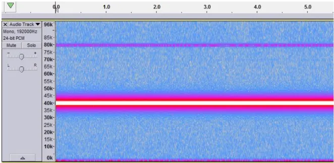
Figure 36 – Received signal of the transmission between the fixed receiver transducer and the transmitter transducer at 20 centimetres.

As shown in the spectrogram of the Figure 36, the transmission was performed with a carrier frequency of 40 kHz. There is power grid noise (50 Hz), which can be seen near the frequency of 0 kHz. In all the experiments performed with the Roland sound card, there was the presence of power in the frequency of 80 kHz. At first, it was thought that it is the second harmonic, which corresponds to the double of the carrier frequency, but changing the carrier frequency would not change the streak at 80 kHz, therefore the assumption that it would be the second harmonic was proved wrong. Transmitting through the inputs of the headphone and the microphone would not generate a streak at 80 kHz, therefore it is assumed that it is caused by the sound card and it will be ignored for analysis purposes.

(67)

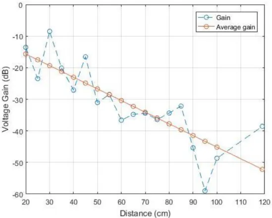
Figure 37 - Gain as a function of distance in the experiment with the fixed receiver transducer. As the gain is not linear, an approximation will be performed with the use of the MATLAB function polyfit. The gain is approximately -36.86 dB/m.

Before analysing this previous experiment, a similar experiment will be described. The following test was performed with the transmitter transducer attached to one end of the pipe, which was filled with water, and the receiving transducer situated at a given distance.

(68)

Figure 38 - Experiment with the fixed transmitter transducer (grey) and the receiving transducer (brown) at a given distance.

Figure 39 - Gain as a function of distance in the experiment with the fixed transmitter transducer.

(69)

As stated in Chapter 3, the theoretical frequency band of the transducers is 39 to 41 kHz. In practice, results showed that the band of frequencies is approximately 39.5 to 41.5 kHz.

The results shown in Figure 37 and Figure 39 do not present a predictable behaviour and its principal reason is the bad mechanical coupling between the transducers and the water pipe. However, the results shown in Figure 37 are considered acceptable, but the results shown in Figure 39 are not good.

With these experiments, it is possible to conclude that the need of having the transducers fixed by a certain connector is indispensable, not only because it provides a better mechanical coupling which is essential for an application in a real piping system, but also because it allows the obtaining of results with robustness. Also, the direction of the wave propagation along the water pipe was not the same as the direction in which it was propagated (according to the orientation of the transducer), which leads to a worse communication, justifying the interest in the next experiments as well.

(70)

4.2.2 Experiment with fixed transducers at the ends of the pipe

Due to the need of using fixed supports for the transducers, it was assembled the following experiment shown in the Figure 40.

Figure 40 - Setup of the experiment with fixed transducers at the ends of the pipe.

The cables assembly shown in the last Chapter were used for this new assembly. The transducers were inserted in the pipe connector, fixed with hot glue and its cables were fixed with adhesive tape as shown in Figure 41, therefore the fixation between the transducer and the connector would not be forced by any intense force applied to the cable. The connectors are made from brass and it is important to note that its internal cavity causes multiple reflections before the signal arrives to the water pipe because the beam pattern is too wide.

(71)

Figure 41 – Transmitter transducer fixed to a pipe connector.

Figure 42 – Receiver transducer fixed to a pipe connector.

The pipe was filled as much as possible and it was performed a signal acquisition. Afterwards, the pipe was changed so it would be possible to test the transmission for a different pipe length. At the receiver there was not the signal sent but power grid noise with

(72)

frequency of 50 Hz. Some tests were performed where the twisting of the pipe connector was relieved, and the pipe was refilled but at the receiver there was always the noise of 50 Hz. After discussing this problem with my mentors, it was decided to construct new cables, which would have the transducers pins accessible to verify if the connections were not broken. This new setup will be presented in the next section.

4.2.3 Experiment with the transducers pins accessible

As stated in Chapter 3, four transducers were bought, therefore, for this experiment it was used the two transducers available, keeping the previous setups for possible further analysis. The new setups are shown in the Figure 43 and in the Figure 44.

(73)

Figure 44 - Receiver transducer.

The disadvantage of this setup is the lack of shielding at the transducers pins since they are not protected by the cable shielding. The unprotected region was wrapped with aluminium foil, however, the received signal was very similar to the one recorded without shielding at the transducers pins, therefore, the aluminium foil did not improve the shielding. In addition, it was also changed the type of piping system used, which before was just one pipe, by adding a male tee connector with a tap (see Figure 45). The purpose of this change was to allow the pipe to be completely filled with water without any air bubbles. It is also important to note that from now, the amplifier will be used.

(74)

Figure 45 - Setup with the 1-meter pipe with a male tee connector in the middle.

After devoting some experiments to the presence and absence of bubbles inside the pipe, it was possible to conclude that the presence of bubbles denies the communication and the signal received is only the power grid noise of 50 Hz. With the presence of bubbles, the transmitted signal is reflected, since the bubbles are an obstacle, causing dispersion, therefore, the communication does not exist. This finding allowed to better understand the acoustic communication inside the pipe and that by eliminating the bubbles, it would be possible to perform the communication.

At this stage of the experiments, it is important to make a pause to think and discuss about the pressure inside the pipe. Considering the transducers were bonded into the pipe connector with silicone, the connection has bad resistance against pressure, therefore, the experiments presented will not take the variable pressure into consideration. It happened twice that the silicone was forced when twisting the pipe connector to an overfilled pipe, which resulted in a displacement of the transducer, therefore a consequent reassembly was needed. To avoid overpressure when tightening the connector to the water filled straight pipe and to work around the problem of the presence of the bubbles, the pipe was drilled and the hole was used for finishing the filling with a syringe. The hole was localized approximately at half of the length of the pipe and had 1mm of diameter. With this method, it was possible to guarantee the absence of bubbles in a straight pipe setup, which does not have a tap.

(75)

Continuing for the following experiment where the peak-to-peak output voltage was registered for various input voltages and for a certain setup. The setups used for this experiment are water filled straight pipe with a length of 0.8 meters (see Figure 46), 1 meter (see Figure 47) and 1 meter with tee connector (see Figure 45 previously shown).

Figure 46 - Setup with the 0.8 meters pipe