ABSTRACT: Aerospace engineering has always had the need for various natural environment parameters to be used as inputs in research and engineering analyses used in the design and development of aircraft and launch/reentry vehicles. Although winds are indeed the main natural environment parameter used as inputs in vehicle design, the thermodynamic atmospheric parameters and models are also of great value and much needed as inputs. This paper will help the design engineer, chief engineer, or project manager understand the role that these thermodynamic parameters/models play.
KEYWORDS: Aerospace meteorology, Launch vehicle development, Mission operations, Atmospheric thermodynamic parameters/models.
Aerospace Vehicle Development
Applications of Atmospheric
Thermodynamic Inputs
William Walton Vaughan1,Dale Leroy Johnson2INTRODUCTION
This paper is a follow-up to the article “Aerospace Meteorology: An Overview of Some Key Environmental Elements”, published in the Journal of Aerospace and Technology Management (Vaughan and Johnson, 2013). It has presented an overview with background on how the natural environment plays a major role in the design and development of launch vehicles, with an emphasis on what is presented in the NASA technical report, “Terrestrial Environment (Climatic) Criteria Guidelines for Use in Aerospace Vehicle Development” (Johnson, 2008), as a help to the design engineer. his paper presents a few speciic examples of how the atmospheric thermodynamic parameters (pressure, temperature and density) along with how thermodynamic model atmospheres play a signiicant role as input in engineering vehicle design and analysis.
Surface and upper air winds are usually the main natural environment driver used in launch vehicle design and development. A launch vehicle’s light control and structural systems are sensitive to extreme wind speed, turbulence, wind gust, and wind shear that may occur during launch and ascent (or lit-of) throughout the Earth’s terrestrial atmosphere (from 0 to 90 km altitude).
However, the three thermodynamic parameters of the atmosphere (pressure, temperature and density) are also very important in aerospace vehicle planning, design, development, testing and launch/reentry. his paper presents a historical look at the use of some of these thermodynamic procedures/models. he NASA Terrestrial Environment (Climatic) Criteria Guidelines Technical Memorandum (Johnson, 2008); hereater referred to
1.University of Alabama – Huntsville/AL – USA 2.NASA (retired) – USA
as TM (Johnson, 2008) has over the years been a major natural environments initial source document. It contains 13 key technical natural terrestrial environment parameters that can be used in the engineering design and development of launch/space vehicles. It presents the surface and in-light thermodynamic parameters of the atmosphere in a statistical and modeling mode. The applicable model should be selected for design use based on the operational requirements for the aerospace vehicle. Mean and extreme values of these thermodynamic parameters can be used in application to many aerospace vehicle design and operational problems, such as (1) research planning and engineering design of remote Earth sensing systems, (2) vehicle design and development, and (3) vehicle trajectory analysis, dealing with vehicle thrust, dynamic pressure, aerodynamic drag, aerodynamic heating, vibration, structural and guidance limitations, and reentry analysis.
Model atmospheres have also been used and improved, starting with use of the U.S. Standard Atmosphere 1976 (Anon., 1976), and its predecessors, for any U.S. site in general. However, if suicient surface and alot atmospheric data (measurements) exist for the exact launch site location, a Range Reference Atmosphere (RRA) can then be developed speciically for that site. Finally a Global Reference Atmospheric Model (GRAM-2010) (Leslie and Justus, 2011), has been developed so that thermodynamic values versus altitude can be obtained for any site on planet Earth. A launch or a re-entry trajectory can also be run through GRAM.
Atmospheric density normally has been the main thermodynamic parameter afecting launch vehicle development for light within the terrestrial environment. Initially, mean or median values of density (from standard or reference atmospheres for a speciic site) were used as input for certain engineering calculations. Extremes of density, i.e. vertical proiles of maximum and minimum have also been used for all altitudes within the terrestrial atmosphere. However, this is very unrealistic in the real atmosphere as density is not an extreme at all terrestrial altitudes. herefore, this brought about the construction of hot (summer) and cold (winter) atmosphere development for the various launch sites of interest to NASA, speciic sites such as Kennedy Space Center (KCS)/FL, Vandenberg Air Force Base (VAFB)/CA, and Edwards Air Force Base (EAFB)/CA, etc. Finally, the NASA MSFC Global Reference Atmospheric Model (Leslie and Justus, 2011) provides in-light atmospheric thermodynamic variables for all global geographical sites.
Another unique thermodynamic procedure developed over the years is also presented within this paper. he Buell statistical relationships (Buell, 1954; Buell, 1970) between the independent
variables of atmospheric pressure (P), temperature (T), and density (ρ) has been developed. his method allows one to obtain simultaneous values of two thermodynamic variables at discrete altitude levels, given that the third variable is an extreme value. Whenever an extreme thermodynamic parameter like ρ is given, the associated P and T values can then be calculated from this statistically developed procedure (equations). Likewise, also for the other two atmospheric thermodynamic parameters, should they be extreme values.
Finally, if meteorological balloon and rocket data exist only up to about 55-km altitude, there is another statistical technique which extrapolates the thermodynamic data from the last level of measurement up to the 90 km terrestrial altitude level, with acceptable accuracy (Graves et al., 1973). his extrapolation procedure is not presented within this paper, but can be obtained directly from Graves, et al.(1973).
he Standard Atmosphere section of TM (Johnson, 2008) presents a more detailed and complete overview of all atmospheric thermodynamic models and procedures than the ones presented here. Most of what is presented in this paper was taken from the Johnson (2008), and much of the description and text presented here has been taken directly from all the various references cited. Keep in mind that the TM (Johnson, 2008) is a terrestrial natural environment engineering applications document that has been maintained and updated by NASA for over the last ity years, as it provides to the engineer or program/project manager all the various natural terrestrial environment statistics and models that can be used in the planning, design and development of aerospace vehicles and payloads.
What is presented within this paper is a discussion of (1) atmospheric density versus altitude, (2) the atmospheric thermodynamic parameters and how they were applied within the Space Shuttle Program design, (3) the Standard and Reference atmospheres, (4) typical hot and cold atmospheres, (5) the Earth Global Reference Atmospheric Model, and (6) the application of the Buell statistical relationships regarding an extreme thermodynamic parameter and the two associated parameters.
DISCUSSION
atmospheric density (surface and at altitude) variability is presented in detail in Johnson (2008). he other key or unique thermodynamic parametric relationships for this paper are discussed below.
IN-FLIGHT ATMOSPHERIC DENSITY AT ALTITUDE
he density of the atmosphere decreases rapidly with height, decreasing to one-half of the surface value at ~7 km altitude at mid latitudes. Density is also variable at a ixed altitude, with the greatest relative variability occurring at ~70 km altitude in the high northern latitudes (60°N). Other altitudes of maximum density variability occur around the surface and 16 km. Altitudes of minimum variability occur around 8, 24 and 90-km altitude. Figure 1 shows these altitude density tendencies for the Kennedy Space Center/FL area along with the extreme density envelope, and hot/cold density values as a percent of the Patrick Reference Atmosphere 1963 (Smith and Weidner, 1964). hese extreme density values approximate the ±3 σ (corresponding to
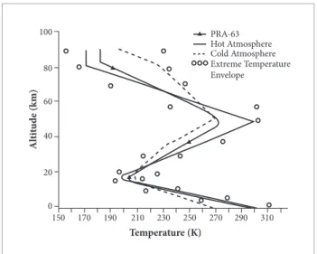
the normal distribution) density values. Figure 2 provides the associated virtual temperature proiles for the KSC extreme, and hot/cold, and PRA-63 Models.
Density varies with latitude in each hemisphere, with the mean annual density near the surface increasing toward the poles. In the region around 8-km altitude in the Northern Hemisphere;
e.g. the density variation with latitude and season is small. Above 8-km to ~28-km, the mean annual density decreases toward the north. Mean monthly densities between 30-km and 90-km increase toward the north in July and toward the equator in January (Smith, 1964; Johnson, 2008). Drag on a reentering spacecrat, which is a direct function of atmospheric density at a given altitude for a speciic vehicle, like the Space Shuttle, has varied up to 19% over a few seconds of light time, resulting from “patchy” density variations (density “pot holes”). he designer must recognize that atmospheric density variations do occur, and they will highly inluence engine performance, speciic fuel consumption, drag, and flight control. GRAM-2010 (Leslie and Justus, 2011) has been designed to reproduce typical density variations that can be encountered along a given light path and should be considered in vehicle design, both ascent and reentry.
THERMODYNAMIC PARAMETER REQUIREMENTS USED IN THE SPACE SHUTTLE PROGRAM
The Space Shuttle Requirements document, NASA NSTS 07700 Book 2, Volume X, Appendix 10.10 (Anon., 1999), contains very speciic atmospheric wind and thermodynamic parametric requirements to use for the design and development of the Space Shuttle launch vehicle. Requirements are given with regard to the atmospheric thermodynamic parameters, as shown in the paragraph below, taken directly from cited document. Key models and purposes are presented. Most of these requirements refer back to the Terrestrial Environment
Figure 1. Relative deviations (%) of extreme KSC density proiles with respect to PRA-63 density. KSC hot & cold density also shown (Johnson, 2008).
120
100
80
60
Al
ti
tu
d
e (k
m)
40
20
0
(%)
-30 -20 -10 0 10 20 30
Envelope of Maximum and Minimum Density
COLD HOT
Figure 2. Extreme KSC virtual temperature proiles and the KSC hot & cold temperatures shown with the PRA-63 Temperature (Johnson, 2008).
100
80
60
Al
ti
tu
d
e (k
m)
40
20
0
Temperature (K)
150 170 190 210
PRA-63 Hot Atmosphere Cold Atmosphere Extreme Temperature Envelope
(Climatic) Criteria Guidelines document of 1973 (Daniels, 1973), which was base-lined early-on for the Space Shuttle program. Since the Earth GRAM was not developed when the Shuttle Requirements Document (Anon., 1999) was irst assembled, it was not included initially.
NASA NSTS 07700 (Anon., 1999), contains the neutral atmosphere requirements. he following atmospheric models are base-lined for the Space Shuttle as indicated for the following engineering functions:
• NASA-GRAM: used in Vehicle Design (for Ascent/for Reentry, except at lower altitudes) along given light path; used as subroutine in TRAJECTORy, ORBIT PROPAGATOR, or SIMULATIONS of IN-FLIGHT programs.
• NASA-Hot & Cold Atmospheres: used in ASCENT DESIGN for all ALTITUDES; used in REENTRy STUDIES from 30 km to SURFACE; used in DESIGN CALCULATIONS (aerodynamic heating, engine performance, and ferry operation); used for aerospace ferrying vehicles, in conjunction with hot or cold day design ambient air temperatures over runways, producing the extreme atmosphere resulting in the maximum vehicle design requirement.
• Cape Kennedy Reference Atmosphere (PRA-63): used as NOMINAL CRITERIA for SURFACE to ORBIT INSERTION, ABORT TRAJECTORy and ANALySES for LAUNCHES; used as nominal criteria 30 km altitude to surface, for vehicle reentry; used for return to landing site (RTLS), and EXTERNAL TANK analysis and disposal design. • Buell Extrapolation Technique: used for design
analyses requiring a knowledge of the two atmospheric variables that are associated with a third extreme variable at discrete altitudes.
• U.S. Standard Atmosphere 1976: used as a STANDARD DAy for purposes of ENGINE RATINGS and COMPARISONS THEREOF (SEA level values); used in ORBITER ENTRy (90 km down to 30 km altitude); used for non-RTLS EXTERNAL TANK analysis and disposal design.
STANDARD ATMOSPHERE
A standard atmosphere is a vertical description of atmospheric temperature, pressure and density that is usually established by international agreement and taken to be representative of the Earth’s atmosphere. he irst standard atmospheres established by international agreement were developed in the 1920s, primarily for the purposes of pressure altimeter calibrations and aircrat performance calculations. Later, some countries,
notably the United States, also developed and published standard atmospheres. he term standard atmosphere has, in recent years, also been used by national and international organizations to describe vertical descriptions of atmospheric trace constituents, the ionosphere, aerosols, ozone, atomic oxygen, winds, water vapor, planetary atmospheres, etc. (Vaughan, 2010).
he standard sea-level values of temperature, pressure, and density that have been used for decades are: temperature of 288.15 K, or 15°C; pressure of 1013.25 mbar or 760 mmHg; and density of 1225.00 g/m3 (Anon., 1976).
he history of standard and reference atmospheres are presented and summarized in Vaughan (2010). Key atmospheric engineering models are given in Johnson (2008). he 1966 U.S. Standard Atmosphere Supplements (Anon., 1966) present diferent latitudinal atmospheres for the United States. It includes tables of temperature, pressure, density, sound speed, viscosity, and thermal conductivity for ive northern latitudes (15, 30, 45, 60, 75 degrees), for summer and winter conditions.
REFERENCE ATMOSPHERES
he term reference atmosphere is used to identify vertical descriptions of the atmosphere for speciic geographical locations or globally, such as the Range Reference Atmospheres (RRA) and the Earth-GRAM-2010 version 2 (Leslie and Justus, 2011). hese RRA were developed by organizations for speciic applications, especially as the aerospace industry began to mature ater World War (Vaughan, 2010).
• Argentia, Newfoundland (St. Johns Airport) • Ascension Island, Atlantic
• Barking Sands, Hawaii (Lihue) • Cape Canaveral, Florida
• China Lake Naval Air Weapons Center, California • Dugway Proving Ground (Salt Lake City), Utah • Edwards Air Force Base, California
• Eglin AFB, Florida • El Paso, Texas • Fairbanks, Alaska
• Ft. Huachuca Elec Prvng Grnd (Tucson), Arizona • Great Falls, Montana
• Kwajalein Missile Range, Paciic
• Nimes-Courbessac, France (STS TAL Site) • Nellis AFB, Nevada (Mercury)
• Point Mugu Naval Air Weapons Center, California • Taguac, Guam (Anderson AFB)
• Vandenberg AFB, California • Wallops Island, Virginia (NASA) • White Sands Missile Range, New Mexico
• yuma Proving Ground, AZ (San Diego, California)
A major new feature of the GRAM-2010 (Leslie and Justus, 2011) is the optional ability to use data (in the form of vertical proiles) from a set of RRA as an alternate to the usual GRAM climatology. With this feature, it is possible, for example, to simulate a light proile for an aerospace vehicle that takes of from the location of one RRA site, e.g. EAFB/CA using the range reference atmospheric data to smoothly transition into an atmosphere characterized by the GRAM climatology, then smoothly transition into an atmosphere characterized by a diferent RRA site, e.g. WSMR/NM, to be used as the landing site in the simulation. he user can also prepare data for any other site desired for use in this mode. he GRAM-2010 model will be discussed in more detail later in this paper.
he Patrick Reference Atmosphere (PRA-63) (Smith and Weidner, 1964) is a more extensive site speciic annual reference atmosphere presenting data to 700-km altitude for KSC/FL. Because of the utility of this atmosphere, a simpliied version is given extracted from Johnson (2008). Reference atmospheres are also available for VAFB (Carter and Brown, 1971; Johnson, 2008) and EAFB (Johnson, 1975; Johnson, 2008). hese provide an annual reference atmosphere model to 700 km and have been designated as computer subroutines VRA-71 and ERA-75, respectively.
Currently, some of the most commonly used standard and reference atmospheres used in the U.S. include:
• COSPAR International Reference Atmosphere (CIRA), 1986 • ISO Standard Atmosphere, 1975
• NASA Earth Global Reference Atmosphere Model
(GRAM), 2010
• NRL MSIS Reference Atmosphere, 2000 • RCC/MG Range Reference Atmospheres (RRA) • U.S. Standard Atmosphere, 1976
• U.S. Standard Atmosphere Supplements, 1966
A detailed listing and description of many worldwide reference and standard atmospheric models is given in Vaughan (2010). In 1996, the American Institute of Aeronautics and Astronautics irst published a Guide to Reference and Standard Atmosphere Models (Vaughan, 2010). his document has been updated since then and provides information on theprincipal features for over 70 global, regional, middle atmosphere, thermosphere, test ranges, Earth and planetary referenceand standard atmospheric models.
EXTREME HOT AND COLD ATMOSPHERIC PROFILES FOR KSC, VAFB, AND EAFB
Johnson (2008), gives the two extreme density profiles that correspond to the summer (hot) and winter (cold) extreme atmospheres for KSC, VAFB and EAFB. See Johnson (1973) for VAFB and Johnson (1975) for EAFB, for detailed information pertaining to these extreme atmospheres. The associated values of temperature and pressure versus altitude are also tabulated. These extreme atmospheric profiles should be used in ascent design analyses at all altitudes. For reentry studies, they are to apply only from 30 km to the surface for vehicles to be used at KSC, VAFB, or EAFB. For those aerospace vehicles with ferrying capability, design calculations should use these extreme profiles in conjunction with the hot or cold day design ambient air temperatures. The extreme atmosphere producing the maximum vehicle design requirement should be utilized to determine the design.
large positive deviations of density occur at the surface, correspondingly large negative deviations will occur near 15-km altitude and above. Such a situation occurs during the winter season (cold atmosphere). The reverse is also true — density profiles with large negative deviations at lower levels will have correspondingly large positive deviations at higher levels. This situation occurs in the summer season (hot atmosphere) and is presented in Fig. 1.
he two extreme (hot & cold) KSC density proiles of Fig. 1 are shown as percent deviations from the Patrick Reference Atmosphere, 1963 density proile (Smith and Weidner, 1964). he two proiles obey the hydrostatic equation and the ideal gas law (i.e. the hypsometric relation). he extreme density proiles shown up to 30-km altitude were observed/measured in the atmosphere. he results shown above 30-km altitude are somewhat speculative because of the limited data from that region of the atmosphere. Quasi-isopycnic levels (levels of minimum density variation) are noted at approximately 8 and 86-km. Another level of minimum density variability is seen at ~24 km, and levels of maximum variability occur at zero, ~15 and ~68-km altitude. he associated extreme hot and cold virtual temperature proiles for KSC are given in Fig. 2. Temperatures below ~10-km altitude are virtual temperatures. Virtual temperature includes moisture to avoid computation of the speciic gas constant for moist air (Johnson, 2008).
NASA-MSFC EARTH GRAM-2010
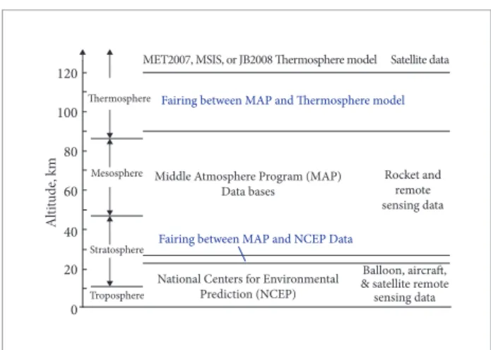
Reference or standard atmospheric models have long been used for design and mission planning of various aerospace systems. The NASA Marshall Space Flight Center Global Reference Atmospheric Model (Leslie and Justus, 2011) was developed in response to the need for a design reference atmosphere (using empirical data bases) that provides complete global geographical variability and complete altitude coverage (surface to orbital altitudes), as well as complete seasonal and monthly variability of the thermodynamic variables and wind components. Figure 3 provides a graphical summary of the data sources and height regions of GRAM-2010. In addition to providing the geographical, height, and monthly variation of the mean atmospheric state, it includes a perturbation model that has the ability to simulate spatial and temporal perturbations in these atmospheric parameters, if dispersions are desired (e.g., fluctuations due to turbulence and other atmospheric perturbation phenomena). When a large number of Monte
Carlo type model profile dispersions are generated at any location, the mean and standard deviation of these data will match those of the observations. The model is statistically equivalent to available measurements. The
±2 σ envelopes encompasses ~95.45% of the observations,
while ±3 σ encompasses ~99.73% of the observations
(according to the normal distribution). This perturbation feature makes Earth GRAM especially useful for Monte Carlo dispersion analyses of guidance and control systems, thermal protection systems, and similar applications. Some of these applications have included operational support for Space Shuttle entry, flight simulation software for other vehicles, entry trajectory and landing dispersion analyses for the Stardust and Genesis missions, planning for aero-capture and aero-braking for Earth-return from lunar and Mars missions, 6 degree-of-freedom entry dispersion analysis for the Multiple Experiment Transporter to Earth Orbit and Return (METEOR) system, and the Crew Exploration Vehicle (CEV). GRAM can also input a spacecraft trajectory and output the various atmospheric parameters along this trajectory path.
The atmospheric model recommended for all reentry analyses, except lower altitudes speciied in Johnson (2008), is GRAM-2010 (Leslie and Justus, 2011). GRAM is also suitable for use as a subroutine in a trajectory code or orbit propagator program or other programs used for simulations of in-light or on-orbit atmospheric variability in density, temperature, or winds.
Figure 3. Summary of the three atmospheric regions in the GRAM-2010 program, sources for the model, and data on which the mean monthly GRAM-2010 values are based. See GRAM-2010 for more details (Leslie and Justus, 2011).
120
100
80
60
A
lt
it
ude
, k
m
40
20
Middle Atmosphere Program (MAP) Data bases
0
Thermosphere
Mesosphere
Stratosphere
Troposphere
MET2007, MSIS, or JB2008 Thermosphere model Satellite data
Fairing between MAP and Thermosphere model
Fairing between MAP and NCEP Data
Rocket and remote sensing data
National Centers for Environmental Prediction (NCEP)
GRAM TRAJECTORY/RE-ENTRY EXAMPLE
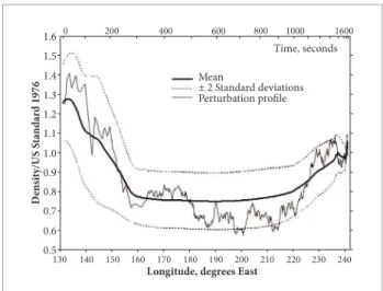
Figure 4 presents a typical re-entry spacecrat trajectory plot of its latitude-longitude location with height and time as indicated. De-orbiting in from a 57°inclination orbit to land at EAFB, in January. Figure 5 shows this same typical trajectory passing through the GRAM-99 derived mean January cross-sectional map of density as a function of height (altitude) vs. longitude (shown as a ratio of U.S.76 Standard density). h e density variability along the trajectory starts at ~20% higher density than the U.S.76 Standard, then goes into a region of ~25% lower than standard, and i nally ~5% higher than standard before landing at Edwards. Figure 6 presents
the same trajectory, and density results, as before; but now includes one Monte Carlo type density perturbation run along this trajectory. This time the trajectory is plotted showing the mean calculated GRAM-99 density, along with the ±2 σ
densities, and the one perturbed density track, all plotted on a density ratio versus longitude graph. Note that the perturbed density does exceed the +-2 σ boundary from time to time, as ±2 σ represents approximately 95.45% of the observations,
according to the normal distribution.
SIMULTANEOUS VALUES OF KSC TEMPERATURE, PRESSURE, AND DENSITY AT DISCRETE
ALTITUDES
h is section presents simultaneous values of atmospheric temperature, pressure, and density as guidelines for aerospace vehicle design considerations. h e necessary assumptions and the lack of sui cient statistical data samples restrict the precision with which these data can currently be presented. h e analysis is currently limited to KSC, FL only. h e Buell (Buell, 1954; Buell, 1970) statistical relationships between atmospheric P, T, and ρ, when 1 is an extreme value, are presented here.
Method of Determining Simultaneous Values
An aerospace vehicle design problem that often arises in considering natural environmental data is stated by the
Figure 4. January Ground Track of a Typical Re-entry Trajectory (57° Inclination Orbit) Landing at Edwards AFB, CA).
40 35 30 L a ti tu d e, d eg re es N o rth 25 20 15
150 160 170 180 190 200 210 z=90km
Circles every 10 km in height Tick marks every 100 seconds
220 230 240 250 260 130 140
45 50 55
Longitude, degrees East
z=120km t=500s z=80km t=1000s z=70km t=1500s t=0
Figure 5. Typical trajectory through GRAM-99 Mean January Height versus Longitude Cross Section of Density (as ratio of US 76 Standard Density).
50 40 30 H eig h t, K m 20 10 0
150 160 170 180 190 200 210
0.90
220 230 240 130 140
60 70 80
Longitude, degrees East 0.80 1.15 1.20 0.75 1.10 1.00 90 100 110 0.95 1.05 0.85 0.95 1.05 1.00 0.90 0.95 0.90 1.00 1.05 1.00
Figure 6. Typical trajectory through GRAM-99 Mean January Atmospheric Density with ±2 s Density Envelopes
(95.45%) and one Monte-Carlo Density Perturbation Proi le
versus Longitude (as a Ratio of US76 Standard Density).
1.0 0.9 0.8 D en si t y/ U S S ta nd ar d 1 9 7 6 0.7 0.6 0.5
150 160 170 180 190 200 210 220 230 240 130 140
1.1 1.2 1.3
L on gitude, degrees E ast
1.5 1.6
1.4
200 400 600 800 1000 1600 0
Mean
Time, seconds
Table 1. Associated Parameters for Extreme Density, Temperature, and Pressure (Johnson, 2008).
Use + sign when extreme parameter is maximum and use – sign when extreme parameter is minimum. M is the 1, 2, or 3 sigma (normal) for the extreme parameter in question.
For Extreme Density For Extreme Temperature For Extreme Pressure
Passoc.
Tassoc.
ρassoc.
following question: “How should the extremes (maxima or minima) of temperature, pressure, and density be combined (1) at discrete altitude levels and (2) versus altitude?” As an example, suppose one wants to know what temperature and pressure should be used simultaneously with a maximum density at a discrete altitude. From statistical principles set forth by Buell (1970), the solution results by allowing mean density plus three standard deviations to represent maximum density and using the coefficients of variations, correlations, and mean values as expressed in Eq. 1 below (Johnson, 2008):
(1)
The associated values for pressure and temperature are the last two terms of Eq. 1, (A) and (B), multiplied by and , respectively, and then this result is added to and , respectively. Appropriate values of the thermodynamic correlation coefficients (r) and coefficients of variation (CV) are obtained from Johnson (2008).
In general, the three extreme ρ, P, and T equations of interest are:
(2)
(3)
(4)
where M denotes the multiplication factor to give the desired deviation. The values of M for the normal distribution and the associated percentile levels are shown in Johnson (2008). h e two associated atmospheric parameters that deal with a third extreme parameter are listed in more detail in Table 1.
It must be emphasized that this procedure is to be used at discrete altitudes only, and holds for a specii c site (KSC FL). Whenever extreme vertical proi les of pressure, temperature, and density are required for engineering application, the use of these correlated variables at discrete altitudes is not satisfactory. In TM (Johnson, 2008) there is a section (hot and cold atmospheres) that deals directly with this problem, since proi les of only extreme values of pressure, temperature, or density at every level from zero to 90-km altitude is unrealistic in the real atmosphere. GRAM can also be used to represent by Monte Carlo process the respective range of thermodynamic parameters for a given geological site.
Table 3. Patrick Reference Atmosphere 1963 (PRA-63) Annual Thermodynamic Parameters of T, P, and ρ at 18 km altitude (from Johnson, 2008).
Altitude (km)
Mean Temperature
(K)
Mean Pressure
(mb)
Mean Density (kg/m3)
0 296.68 1017.01 1.18355
18 205.30 78.0974 0.132392
(5)
and
(6)
And, for Extreme High Summer time Density at 18 km:
(7)
h e following example is shown for the KSC 18-km altitude level during a hot summer day when the surface value of temperature is high (hot) and surface density low. Whereas the value of temperature at the18-km (tropopause) altitude level is very low (cold) while the atmospheric density is very high. To compute the Eqs. 5 and 6 values for the associated density and pressure for this KSC extreme case of low (cold) temperature at 18-km altitude, one just needs to insert the thermodynamic CV and r values from Table 2 into Eqs. 5 (and 6) of Table 1. h e associated value of 18-km density then turns out to be:
ρassoc. = 0.132392 [1 -{ 3 (0.0275) (-0.7904)}] or
ρassoc. = 0.141025 kg/m3
Which gives a higher density value than the annual PRA-63 density value does at 18-km. h e percentage is 6.5% greater than the PRA-63 18-km density value (from Table 3).
ρPRA63
∆ρ = ρmax or min - ρPRA63 x 100 %
(8)
Next, the associated value for pressure at 18 km, from Eq. 6, is calculated as follows:
Passoc.=78.0974 [1-{ 3 (0.0175) (-0.2706)}] or
Passoc=79.20689 mb
Which is 1.4% greater than the PRA-63 18-km pressure value at 18 km altitude.
Next, we should compute the calculated low temperature value at 18 km altitude, given a high value maximum density condition at that same altitude level. So, using Eq. 7, for a given high density extreme, we can compute the associated value of temperature as follows:
Tassoc=205.3 [1+{ 3 (0.0170) (-0.7904)}] or
Tassoc=197.02 K
Which is -4.0% of the PRA-63 temperature value at 18-km altitude.
Finally, we should determine if these calculated values of associated density, pressure, and temperature, given an extreme parametric condition at 18-km altitude (i.e. extreme low temperature, extreme high density), are close to reality or not. We have obtained a few extremely hot summer day vertical sounding measurement taken at KSC. One sounding in particular (June 16, 1958) is very extreme at the surface (hot temperature) and at 18-km altitude (cold temperature), as presented in Table 4. By the way, this sounding was one of the key soundings used in the derivation of the KSC Hot atmosphere.
Comparing the Buell calculated values of associated pressure, temperature and density at altitude of 18 km with the measured observations (Radiosondes-Raob) values gives good results as shown in Table 5. h e three parametric value percent dif erences Atmospheric deviations as a percentage from the
annual PRA-63 were computed by the following Eq. 8 (only density shown):
Table 2. KSC atmospheric thermodynamic coefi cients of variation (CV) and correlation coefi cients (r) between P, T, and ρ, at 18-km altitude (from Johnson, 2008).
CV (%)
[σ
ρ/ ] [σP/ ] [σT/ ]
2.75 1.75 1.70
(r )
r(Pρ) r(PT) r(ρT)
0.8036 -0.2706 -0.7904
REFERENCES
Anon., 1966, “U.S. Standard Atmosphere Supplements, 1966”, U.S. Government Printing Ofice, Washington, DC, 1966, pp. 3-36.
Anon., 1976, “U.S. Standard Atmosphere, 1976”, U.S. Government Printing Ofice, Washington, DC, October 1976.
Anon., 1984, “Range Reference Atmosphere Documents” published by Secretariat, Range Commanders Council (RCC), Meteorology Group (MG), White Sands Missile Range, NM.
Anon., 1999, “NASA NSTS 07700 Natural Environment Space Shuttle Flight and Ground System Speciication, Book 2, Vol. 10, Apx. 10.10”.
Buell, C.E., 1954, “Some Relations Among Atmospheric Statistics”, Journal of Atmospheric Sciences, Vol. 11, No. 3, pp. 238-244.
Buell, C.E., 1970, “Statistical Relations in a Perfect Gas”, Journal of Applied Meteorology, Vol. 9, No. 5, pp. 729-731.
Carter, E.A. and Brown, S.C., 1971, “A Reference Atmosphere for Vandenberg AFB, California, Annual (1971 Version),” NASA/TM X–64590, NASA Marshall Space Flight Center, AL.
Cole, A.E. and Kantor, A.J., 1978, “Air Force Reference Atmospheres”, AFGL–TR–78–0051, Air Force Surveys in Geophysics, No. 382.
Daniels, G.E., 1973, “Terrestrial Environment (Climatic) Criteria Guidelines for Use in Aerospace Vehicle Development, 1973 Revision”, NASA/TMX-64757.
Graves, M.E., Lou, Y.S. and Miller, A.H., 1973, “Speciication of Mesospheric Density, Pressure, and Temperature by Extrapolation”, NASA/CR-2223, March 1973. Retrieved in January 23, 2013,from http://ntrs.nasa.gov/archive/nasa/casi.ntrs.nasa. gov/19730012637_1973012637.pdf
are all within 0.8% of the measured Raob values. his is to be expected due to the fact that the inter- and intra-level correlations are very high at and between the surface level and the tropopause level for temperature and density.
SUMMARY REMARKS
This paper presents some of the function and use that atmospheric thermodynamic parameters of pressure, temperature and density have had in the design and development of aerospace launch and reentry vehicles for flight through the terrestrial atmosphere. The application and use of these atmospheric models, or statistical values, will help the program/project managers and engineers with useful atmospheric inputs for engineering design, usage and trade studies. Most of the information presented here came from (Johnson and Vaughan, 2012) and especially (Johnson, 2008).
Table 5. Calculated versus KSC Measured Values of T, P, and ρ at 18 km altitude.
Calculations Temperature Pressure Density
PRA-63 values 205.30 K 78.09740 mb 0.132392 kg/m3
Buell Computed (% of PRA-63) 197.02 K 79.20689 mb 0.141025 kg/m
3
-4.0 % +1.4 % +6.5 %
Raob Measured (% of PRA-63) 195.50 K 79.77020 mb 0.142200 kg/m
3
-4.8 % +2.1 % +7.4%
KSC-Hot values (% of PRA-63)
200.0 K 81.36950 mb 0.141732 kg/m3
-2.6 % +4.2 % + 7.1 %
(% of Computed from Measured) +0.78 % -0.71 % -0.83 %
Table 4. Actual KSC Atmospheric Raob Sounding Measurement for 1958-06-16-00Z.
Altitude (km)
Temperature (K)
Pressure (mb)
Density (kg/m3)
Sfc. 307.46 1010.00 1.1366
Johnson, D.L., 1973, “Hot and Cold Atmospheres for Vandenberg AFB, California (1973 Version)”, NASA TM–64756, NASA Marshall Space Flight Center, AL.
Johnson, D.L., 1975, “Hot, Cold, and Annual Reference Atmospheres for Edwards Air Force Base, California (1975 Version)”, NASA/TM X–64970, NASA Marshall Space Flight Center, AL.
Johnson, D.L., 2008, “NASA/TM-2008-215633 Terrestrial Environment (Climatic) Criteria Guidelines for Use in Aerospace Vehicle Development, 2008 Revision”, Dec. 2008. Retrieved in January 23, 2013, from http://ntrs.nasa.gov/archive/nasa/casi.ntrs.nasa. gov/20090022159_2009021428.pdf
Johnson, D.L. and Vaughan, W.W., 2012, “How Atmospheric Thermodynamic Parameters and Model Atmospheres Have Been Used to Help Engineering in Aerospace Launch Vehicle Design & Development”, 50th AIAA 2012 Aerospace Sciences Meeting, Nashville, TN.
Leslie, F.W. and Justus, C.G., 2011, “The NASA Marshall Space Flight Center Earth Global Reference Atmospheric Model-2010 Version 2”, NASA/TM—2011–216467.
Smith, J.W., 1964, “Density Variations and Isopycnic Layers”, Journal of Applied Meteorology, Vol. 3, No. 3, pp. 290-298.
Smith, O.E. and Weidner, D.K., 1964, “A Reference Atmosphere for Patrick AFB, Florida, Annual (1963 Revision)”, NASA/TM X–53139, NASA Marshall Space Flight Center, AL.
Vaughan, W.W., 2010, “Guide to Reference and Standard Atmospheric Models”, AIAA G-003C-2010, American Institute of Aeronautics and Astronautics, Reston, VA.