ABSTRACT: The noise source distribution of a short-cowl coaxial jet operating at different velocity ratios is described in this work. This was motivated by an ongoing research about noise prediction of coaxial jets through Acoustic Analogy with purposes of industrial engine application. This research has been carried out between Universidade Federal de Uberlândia (UFU), Brazil and the Institute of Sound and Vibration Research (ISVR) at Southampton University, UK. The numerical approach employed is originally based on Lighthill Acoustic Analogy. This technique, although likely known, is associated with an improved energy transfer time-scale, used in the turbulence two-point correlation function, in order to enhance the source model. The source model is coupled with the aerodynamic calculation of low through turbulence quantities evaluated by using a standard k-ε turbulence modeling. The Computational Fluid Dynamics data have also been used to provide complementary information about the coaxial jet noise production mechanisms. Experimental data were used in order to corroborate the results from the current model. Good agreement has been found, showing that high and low frequency contributors to the radiated noise for low velocity ratio are aggregated in a region about seven to ten secondary diameters downstream, while at higher velocity ratios sources are continuously spread from about one up to ten secondary diameters from the jet exit.
KEYWORDS: Aeroacoustics, Acoustic analogy, Turbulence, Noise, Nozzle.
Noise Source Distribution of Coaxial
Subsonic Jet-Short-Cowl Nozzle
Odenir de Almeida1, João Roberto Barbosa2, Juan Battaner Moro3, Rodney Harold Self3
INTRODUCTION
Measuring and locating noise sources in jet lows is doubtless a diicult task since it requires special equipments and reined techniques. However, the understanding of noise production and radiation mechanisms in these lows would perfectly hold up by such achievement. Indeed, knowing exactly all the patterns behind the sources of jet noise and their location would lead towards a new phase of developing noise suppression devices and optimization of diferent concepts for industrial applications, for example, aero-engines.
One of the most common methods for investigating the noise radiated by a jet low is the determination of the source strength distribution along the jet axis. For single jet lows, this has been experimentally done by diferent techniques, using microphone phase array system and/or by using a highly directive microphone system like an elliptic mirror (Laufer et al., 1976; Fisher et al., 1977; Harper-Bourne, 1999).
he problem of noise source distribution intensiies when considering coaxial jets due to the nature or structure of the coaxial low and mainly because the introduction of a number of additional variables, such as area ratio (AR), velocity ratio (VR) and temperature ratio (TR). Nevertheless, many experimental works were set in the last years in order to provide source location data of such lows (Battaner-Moro, 2003; Femi and Bridges, 2004). Concomitantly, numerical research has been evolved through some diferent approaches in order to overcome the lack of information in this ield (Groschel et al., 2006; Tinney et al., 2006; Eschricht et al., 2008).
One of the irst works towards the use of acoustic analogy in order to evaluate noise sources is attributed to Ribner (1958).
1.Universidade Federal de Uberlândia – Uberlândia/MG – Brazil 2.Instituto Tecnológico de Aeronáutica – São José dos Campos/SP – Brazil 3.University of
Southampton – Southampton/United Kingdom
Author for correspondence: Odenir de Almeida | Avenida João Naves de Ávila, 2.121 – Santa Mônica | CEP 38.408-100 Uberlândia/MG – Brazil | Email: [email protected]
Despite the work was quite simple, the most important inding was that the overwhelming bulk of the jet noise is emitted in the region of eight up to ten nozzle diameters downstream the jet exit plane. Chen (1976), also presented a simple analytical model for predicting sound power spectra density of coaxial jets at ambient temperature. It is shown that for coaxial jets the sound source strength distribution along the jet axis is constant in the initial mixing region, decaying like x-7 in the fully turbulent region.
Based on the Lighthill (1952) acoustic analogy, Self (2004) introduces a jet noise source model in which a new feature is taken into account that is the inclusion of frequency dependence for the time and length scales used in the turbulence two-point correlation function. It is found that allowing for this dependence markedly improves the agreement of the prediction of the model with experimental data. his model has been utilized to describe the noise source distribution in a subsonic single jet with potential to other applications.
hus, an extension of this model is presented in this work as part of an ongoing research about noise prediction of coaxial jet through acoustic analogy. Clearly, the source model can be generalized to use Reynolds Averaged Navier-Stokes (RANS) and other Computational Fluid Dynamics (CFD) data to predict jet noise, for single and coaxial jets and also for more novel nozzle geometries. Based on that, the main goal was to identify and quantify noise sources for coaxial jets for industrial application, through the development of a simpler model, which predicts the source noise distribution mainly based on simple turbulence scales quantities. Although the approach may be simplistic from the acoustic and low interaction standpoint, since the predictions are limited to 90° to the jet axis, the source model shows promising results and contribute for the physical understanding of noise generation, being useful to address practical problems in industry.
he mathematical modeling is coupled and processed with the aerodynamic low computation by turbulence quantities like turbulent kinetic energy (k) and turbulent dissipation rate (ε). hese quantities have been calculated by using CFD RANS approach with a standard k-εturbulence model – such details are given in sections; Acoustic model, he polar correlation technique, Test article and operating conditions and Computational luid dynamics. he CFD simulations in this work were employed with two fold purposes: irst, to provide turbulence quantities to the acoustic model and, second, to give support in understanding the jet noise production mechanism
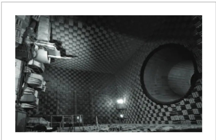
through the analysis of the pattern of the turbulence in the low over diferent operating conditions. he numerical results were compared against experimental data collected from Coaxial and Jet Noise (CoJeN) project (European Union Research Programme – FP6), which undertook several measurements of various types of coaxial nozzles at diferent working conditions. he experimental validation data is available from the work of Battaner-Moro, carried out in 2008 (not published yet), which undertook coaxial jet source location measurements using the Polar Correlation Technique (Battaner-Moro, 2003). hese measurements were performed at QinetiQ’s Jet Noise Facility in Farnborough, UK, and consist of source images and frequency distribution. his large facility (Fig. 1) is able to generate model-scale cold and hot jets in an anechoic environment.
ACOUSTIC MODEL
In this section, the acoustic model is described. The mathematical model for jet noise source distribution is based on the Lighthill acoustic analogy as shown in the following equations. In order to make predictions of the noise for coaxial jet lows, it is necessary to couple the acoustic model to CFD-turbulence results as an input for the source modeling. It is important to emphasize that although the Lighthill acoustic analogy includes convective ampliication efects, such theory will not itself account for low-acoustic interaction. his means that an accurate prediction of the far-ield pressure distribution is limited to an angle of 90° to the jet axis, in which such efects are unimportant.
he model itself is quite simple and easy to be numerically implemented. he whole mathematical description will not be presented herein and additional details about the mathematical formulation can be seen in Self (2004). he overall intensity as an integral over the axial extent of the jet is considered according to Eq. 1:
(1)
where Ix is the overall sound intensity, R is the radial distance,
w is the angular frequency and x is the microphone distance.
Following Goldstein (1976), Eq. 1 deines the axial source distribution for a speciic frequency (w) at any radial distance (R). Since the aim is to identify the source distribution for a 90° observer, the following relation can be readily found from Lighthill’s equation:
(2)
where Ln are the characteristic correlation length scales in the three axial directions, characterizing the size of the eddies. In this case it is assumed L1 = L2 = L3. he time-scale is represented by t and u is a velocity characteristic of the turbulence. he angular frequency, 2πƒ, is represented by w, c0 is the mean sound speed,ϕ is the azimuthal location and r is the radial location.
As it has been pointed out by several authors, a crucial factor for describing the turbulence in a flow is t. The definition of t in the current model plays an important role for predicting the location and the contribution in the frequency range. It has been shown by experiments of Harper-Bourne (1998), that both length and time-scales are frequency dependent, which means that for a good spectrum prediction such dependence must be taken into account. The frequency dependence in both length and time-scales can control both the location of the peak-frequency and also the shape of the spectrum at higher frequencies.
In this work, an energy transfer time-scale (TET) has been used in order to enhance the predictions in the source model. his time-scale that is based on the transfer of turbulent energy between diferent wave numbers of the turbulent luctuations is associated with the inertial sub range where the noise production mechanism is largely governed by the energy transfer phenomenon.
hus, t in Eq. 2 assumes the following relation (Azarpeyvand et al., 2006):
(3)
where aT is an empirical constant that must be adjusted. his
coeicient aTis currently utilized to correct the shape of the
spectrum and set the peak frequency location. A complete study about the inluence of this factor aTwas presented in
Almeida (2009). In this work, a range of values aT= [0.38 – 0.45]
was applied showing satisfactory results. hese values are in agreement with the work of Almeida (2009). In Eq. 3, td is
the traditional time-scale based on the turbulence decay rate k/ε. Λ denotes the size of the eddy which can be either found from experimental results or be estimated. In this work, a range of values of Λ=[1.8 – 2.0] has been used. Finally, l is the length-scale, as deined by:
(4)
Equation 4 gives the values for L1 = L2 = L3. It is important to observe at this time that a model for anisotropy could be taken into account to describe the relationship among the three axial directions. he use of the TET time-scale has provided a good agreement with the experimental results, showing a more physically realistic shape of source distribution.
he acoustic model presented herein is fed in with CFD RANS results. Both t and l are evaluated by using k and ε values provided by the aerodynamic simulation of the subsonic low through a short-cowl nozzle as seen in aero-engines. Details of CFD simulations and analysis of results will be described in section Computational luid dynamics.
THE POLAR CORRELATION
TECHNIQUE
and an equivalent line-source strength distribution (S) along the jet axis y (Fig. 2). For an array of incoherent sources, the following relation holds:
(5)
where a is the polar angle from the reference microphone at 90°. In principle,
(6)
his Fourier relationship holds for uncorrelated far ield sources. he following assumptions can then be taken: 1 he distances from each source to the jth microphone r
j (y)
and to the reference microphone rref (y) are equal to the array radius, i.e. rref (y) = rj (y) = r.
2 All the source/microphone angles are equal, i.e. for the directivity terms di (θj (y)) = di (θref (y)) = constant. 3 he phase term, rref (y)– rj (y) may be approximated by y
sin (aj).
It is important to emphasize that successful polar correlation imaging is based on careful consideration to the design of the microphone array. This design must take into account
the characteristics of what are going to be measured and the frequency of interest. his is so because all practical microphone array techniques are subjected to geometric constraints which limit the available resolution and introduce undesired spatial aliasing. For the CoJeN nozzle, a ± 30° aperture microphone polar array with 63 microphones was used, as detailed in Table 1. Further details about the experimental setup can be found in Battaner-Moro (2003).
he microphones are positioned downstream the nozzle exit, covering a spherical arc, and numbered as described on Table 1 and Fig. 2.
SOURCE IMAGES
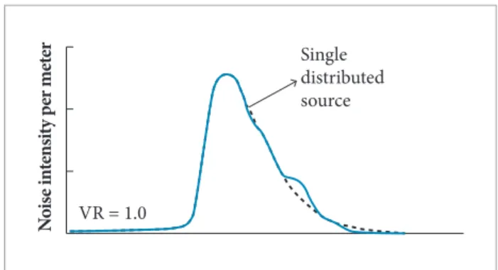
The experimental approach by using Polar Correlation Technique provided source images assumed to be in the form of a line distribution and the noise intensity/meter of both the measured and the fitted data are plotted as a function of axial distance along the centerline of the jet. Figure 3 is an example, in which the measured image, obtained by taking a Fourier transform of the measured coherence data, is shown as a solid line. When source images of model coaxial exhaust jets were first studied, an important phenomenon was observed. Over a wide frequency range, the images were seen to display a double peak (Strange et al., 1984). This double peak phenomenon was seen consistently over a range of coaxial nozzles of different size, showing the presence of a secondary source downstream the jet.
Further investigation, as presented by literature, showed that the appearance of this secondary downstream source was strictly related to the low aerodynamics and the velocity ratio parameters. As presented by Strange et al. (1984), for a coaxial low at velocity ratio equal to 1, only a single distributed source appears in the image. The emergence of the downstream source from its subdominant role, at a velocity ratio of 0.8, to the dominant source, at a velocity ratio of 0.62, gives a very clear indication that what is being observed in the source image is closely related to the low conditions.
Table 1. Polar microphone array angular spacing (CoJeN).
Mic spacing Mic positions Mic units
0.25° 60° to 64° and 86° to 90° 32 mics
0.5° 64° to 68° and 82° to 86° 16 mics
1.0° 68° to 82° 15 mics
Figure 2. Polar microphone array and equivalent line jet noise source distribution.
1 2
N
y S(y,ω)
αN
α2
TEST ARTICLE AND OPERATING
CONDITIONS
The test article consists of a short-cowl nozzle which is representative of a large modern high bypass ratio aero-engine, assuming a nominally 1/
10
th scale. It has a secondary nozzle diameter of 274.4 mm, followed by a primary nozzle and a centerbody (Fig. 4). he experimental acoustic data used in this section, for comparison purposes, are collected from the CoJeN project (European Union Research Programme – FP6) Contract no. AST3-CT-2003-502790. he current work has been processed at
Figure 3. A typical coaxial jet source image (Strange et al.
1984).
N
o
is
e in
te
ns
it
y p
er me
te
r
VR = 1.0
Single distributed source
Institute of Sound and Vibration Research (ISVR) at Southampton University in 2009 and 2010.
Table 2 presents the low conditions for the coaxial jet lows investigated in this work. Both primary and secondary streams where considered isothermal, i.e. the static temperature in the nozzle exit plane, Tj, is equal to the static temperature of the ambient air, T0. he nozzle operating velocities have been changed to match three diferent velocity ratios VR=1.0, VR=0.75 and VR=0.63. he VR has been deined as the ratio between the secondary and primary stream (Vs/Vp).
COMPUTATIONAL FLUID DYNAMICS
CFD through RANS methodology has been applied in this research in order to provide the mean low quantities necessary to the acoustic model, as shown in section Acoustic model. he turbulence modeling is also a key point in the whole formulation, since quantities like k and ε are used to compute the noise source strength, and is of great importance for understanding the underlying physics of the noise production mechanisms. It is clear that the CFD RANS alone does not reveal the frequency content of the sources. However, it is still possible to interpret CFD results by knowing that the high frequency sources are oten aggregated in the close vicinity of the jet exit (between the potential core and the surrounding medium) and the low frequency sources further downstream (mixing region).
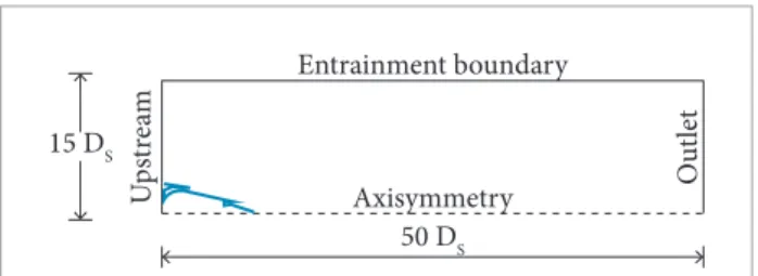
The dual-stream isothermal jets operating at the velocity ratios mentioned in Table 2 have been considered in this study and a RANS scheme using a finite volume scheme with a standard k-ε turbulence model (Launder and Spalding, 1972) was used to calculate the mean and turbulence quantities. The dimensions and boundary conditions for the computational domain used in the RANS simulations are illustrated in Fig. 5. Figure 6 shows part of the short-cowl mesh used for the CFD calculations. For such a kind of approach, there is no need to process a 3D full model, since RANS is only able to provide an average flow-field for the parameters of interest quantities like k and ε. A comparison between 3D and 2D simulations has shown a very good agreement, as presented in Almeida (2009). It must be remembered that the analysis is performed by a noise source distribution in a centerline at the exit plane of the nozzle. Such approach is useful for industry application Figure 4. Short-cowl nozzle geometry.
VS
Vp DS = 0.274 m
Dp = 0.136 m
D
S: secondary diameter; Dp: primary diameter; V
S: velocity at secondary stream; Vp: velocity at primary stream.
Table 2. Operating conditions – isothermal low.
Condition Vp (m/s) Vs (m/s) VR
1 217.2 217.2 1.0
2 217.2 162.9 0.75
3 217.2 136.8 0.63
V
p: velocity at primary stream; Vs: velocity at secondary stream; VR: velocity ratio; P
since it requires less computational power and good results can be achieved. A well-deined axisymmetric 2D simulation is a compromise between time of processing and reasonable low prediction. With modern hardware availability, such analysis could provide results around one and two days of work, being the mesh generation the most complex part of the process.
The final axisymmetric computational domain discretization consisted of a block structured mesh with 12 blocks and a total of 203,942 elements. The mesh points were concentrated to the shear layer region and clustered
in the nozzle wall following a 7th- law turbulent boundary
layer approach in order to provide a Y+ of approximately
30 in the near wall regions. A linear growing law is used to increase the elements in axial and radial direction. A sharper mesh jump is avoided during block transitions. It
is important to mention that, despite the fact that the Y+ is
not too large, some additional tests provided in Almeida (2009), showed the need to include near wall treatment for the short-cowl nozzles simulations.
Figure 6. Short-cowl mesh reinement over the domain – 203,942 quadrilateral elements.
x
y
Figure 5. Computational Fluid Dynamics domain and boundary conditions – short-cowl nozzle (application).
Entrainment boundary
U
p
st
re
am
Ax i symmetry O
u
tlet
15 DS
50 DS
Inlet: total pressure and enthalpy; Entrainment: static pressure and temperature; Outlet: static pressure and temperature; Axis: axisymmetry.
AERODYNAMICS AND SOURCE
DISTRIBUTION RESULTS
he numerical results in this section are separated between the low prediction through RANS simulations and the noise source distribution through the acoustic modeling. he section Aerodynamic Calculation describes the CFD results for diferent
subsonic short-cowl coaxial jet low operating at diferent VR
of 1.0, 0.75 and 0.63, in accordance with Table 2. Following, the section Source distribution presents the predicted noise distribution at each frequency for the cases, respectively.
AERODYNAMIC CALCULATION
Aerodynamic calculations for the short-cowl nozzle
jet operating at the VR mentioned in Table 1 have been
considered in this study by employing a RANS scheme using
a standard k-ε turbulence model to evaluate the mean and
turbulence quantities.
Figure 7 presents the contours of Mach and k for the diferent
VR investigated. It is possible to observe that as the velocity
ratio is close to 1.0 the coaxial jet low resembles a single jet low with the noise source region (high kinetic energy) spread
over two up to ten diameters. As the VR is decreased, it can
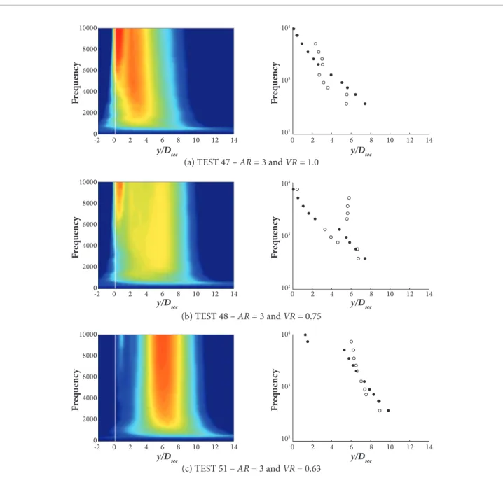
VR=0.75, seems to peak earlier and with a higher frequency. At VR=0.63, the downstream source appears to be more “compact” and peaks at approximately 6 DS. For cases of VR equal to 1.0 and 0.63, the numerical and experimental data agreed satisfactorily. However, a close look on Fig. 9b reveals a discrepancy between experimental and numerical data. he reason for that discrepancy is associated to the presence of some “external” noise content coming either from internal sources in the rig or due to the presence of some solid surface close to the jet. Additional noise tests (experiments) may be necessary to conirm this observation.
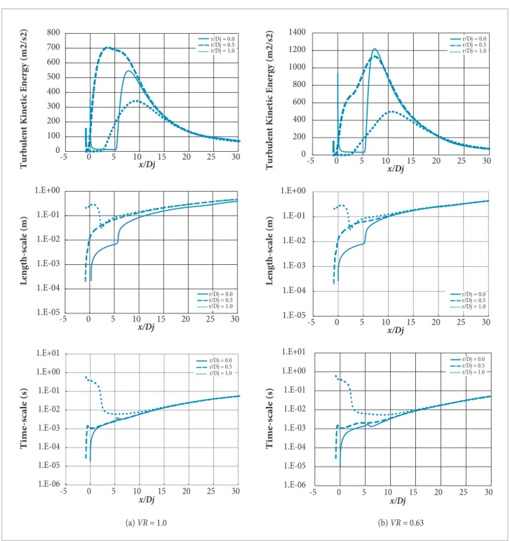
Although the appearance of extra noise sources in the experimental data (it needs further investigation), the numerical location of the sources are reasonably predicted. Such approach is clearly important for study and investigation of regions of diameters. Finally, based on t and l, it can be inferred that the
large structures (big eddies) also start to dominate ater 15 DS.
SOURCE DISTRIBUTION
Figure 9 shows the axial locations of peak of the IX at diferent frequencies for an observer located at 90° and a radial distance of R=65.4 DS. his result indicates a good agreement for the whole range of frequency (200 Hz up to 10 kHz) by using the source model associated with a TET time-scale.
In the let hand side, the contours (images) of the sources can be visualized. On the right hand side, it is illustrated a comparison of the source distribution over a transversal line placed at the origin – line plot. For VR equal to 1 and 0.75, the sources are not well distributed, peaking at diferent axial locations. The second downstream source, appearing for
Figure 7. Mach number (M) (left) and turbulent kinetic energy (k) (right) – short-cowl nozzle (AR = 3).
(a) VR = 1.0
(b) VR = 0.75
(c) VR = 0.63
0.6 0.55 0.5 0.45 0.4 0.35 0.3 0.25 0.2 0.15 0.1 0.05 5 4 3 2 1 0 r/D S x/DS
0 2 4 6 8 10
1200 1000 800 600 400 200 5 4 3 2 1 0 r/D S x/DS
0 2 4 6 8 10
0.6 0.55 0.5 0.45 0.4 0.35 0.3 0.25 0.2 0.15 0.1 0.05 5 4 3 2 1 0 r/D S x/DS
0 2 4 6 8 10
1200 1000 800 600 400 200 5 4 3 2 1 0 r/D S x/DS
0 2 4 6 8 10
5 4 3 2 1 0 0.6 0.55 0.5 0.45 0.4 0.35 0.3 0.25 0.2 0.15 0.1 0.05 0 2 x/DS r/D S
4 6 8 10
1200 1000 800 600 400 200 5 4 3 2 1 0 r/D S x/DS
Figure 8. Flow quantities distribution at different radial locations – short-cowl nozzle (AR = 3; VR = 1.0 and VR = 0.63). In the
plot, the origin (x = 0) is placed at the end of the plug.
(a) VR = 1.0 (b) VR = 0.63
1.E-06 1.E-05 1.E-04 1.E-03 1.E-02 1.E-01 1.E+00 1.E+01
-5 0 5 10 15 20 25 30
x/Dj
Time-scale (s)
1.E-06 1.E-05 1.E-04 1.E-03 1.E-02 1.E-01 1.E+00 1.E+01
-5 0 5 10 15 20 25 30
x/Dj
Time-scale (s)
r/Dj = 0.0 r/Dj = 0.5 r/Dj = 1.0
r/Dj = 0.0 r/Dj = 0.5 r/Dj = 1.0 0
100 200 300 400 500 600 700 800
-5 0 5 10 15 20 25 30
x/Dj
Turbulent Kinetic Energy (m2/s2)
0 200 400 600 800 1000 1200 1400
-5 0 5 10 15 20 25 30
x/Dj
Turbulent Kinetic Energy (m2/s2)
r/Dj = 0.0 r/Dj = 0.5 r/Dj = 1.0
r/Dj = 0.0 r/Dj = 0.5 r/Dj = 1.0
1.E-05 1.E-04 1.E-03 1.E-02 1.E-01 1.E+00
-5 0 5 10 15 20 25 30
x/Dj
Length-scale (m)
1.E-05 1.E-04 1.E-03 1.E-02 1.E-01 1.E+00
-5 0 5 10 15 20 25 30
x/Dj
Length-scale (m)
r/Dj = 0.0 r/Dj = 0.5 r/Dj = 1.0
r/Dj = 0.0 r/Dj = 0.5 r/Dj = 1.0
n oi se source in coaxial jet lows. Especially for a VR=0.63, the numerical source location matched well the experimental results. The final words in this section will be devoted to highlight the potential for using the acoustic model in the source location. However, as previously discussed, the exact
Figure 9. Coaxial source location – short-cowl nozzle; left: image; right: axial source strength/m: (¡) experimental; (l) prediction. (a) TEST 47 – AR = 3 and VR = 1.0
(b) TEST 48 – AR = 3 and VR = 0.75
(c) TEST 51 – AR = 3 and VR = 0.63
Fr
eq
u
en
cy
Fr
eq
u
en
cy
10000
8000
6000
4000
2000
0
10000
8000
6000
4000
2000
0
10000
8000
6000
4000
2000
0
-2 0 2 4 6 8 10 12 14 0 2 4 6 8 10 12 14
104
103
102
104
103
102
104
103
102
y/Dsec y/Dsec
Fr
eq
u
en
cy
Fr
eq
u
en
cy
-2 0 2 4 6 8 10 12 14 0 2 4 6 8 10 12 14
y/Dsec y/Dsec
Fr
eq
u
en
cy
Fr
eq
u
en
cy
-2 0 2 4 6 8 10 12 14 0 2 4 6 8 10 12 14
y/Dsec y/Dsec
B ased on this affirmation and in all the results presented in this work, it is possible to affirm that the acoustic model is promising to deal with coaxial jet flows. However, the model seems to be much more dependent on the aerodynamic results (CFD) when the VR is decreased below 1.0. This is mainly due to the shifting in the noise source location inside the jet plume, which may not be correctly captured with a coarse mesh at downstream positions.
CONCLUSION
main observations were registered as: a) high and low frequency contributors to the radiated noise for low velocity ratio are aggregated in a region about seven to ten secondary diameters downstream, while at higher velocity ratios sources are continuously spread from about one up to ten secondary diameters from the jet exit; b) as the velocity ratio is decreased, the noise sources move downstream the jet axis. his has been corroborated by experimental results. he numerical technique exposed herein is useful for industrial application and can be surely applied to investigate noise source regions in short-cowl nozzles, as seen in modern aircrats.
ACKNOWLEDGMENTS
Prof. Odenir Almeida thanks the financial support provided by Coordenação de Aperfeiçoamento de Pessoal de Ensino Superior (CAPES), Brazil, for the development of this work. He also thanks for all the support received at the Institute of Sound and Vibration for the conclusion of his Ph.D thesis and the Fundação de Amparo à Pesquisa do Estado de Minas Gerais (FAPEMIG).
REFERENCES
Almeida, O., 2009, “Aeroacoustics of Dual-stream Jets with Application to Turbofan Engines”, Ph.D. thesis, Instituto Tecnológico da Aeronáutica, São José dos Campos, Brazil.
Azarpeyvand, M., Self, R.H. and Golliard, J., 2006, “Improved Jet Noise Modeling Using a New Acoustic Time Scale, No.
2006-2598”, 12th AIAA/CEAS Aeroacoustics Conference,
Cambridge, MA, USA.
Battaner-Moro, J., 2003, “Report on Automated Source Breakdown for Coaxial and Single Jet Noise Measurements”, ISVR Internal Report No. 03/10.
Chen, C.Y., 1976, “A Model for Predicting Aeroacoustic Characteristics of Coaxial Jets”, AIAA Paper 76-4.
Eschricht, D., Yan, J., Michel, U. and Thiele, F., 2008, “Prediction of Jet Noise from a Coplanar Nozzle, No. 2008-2969”, 14th AIAA/CEAS
Aeroacoustics Conference, Vancouver, Canada.
Femi, A.A. and Bridges, J., 2004, “Jet Noise Source Localization Using Linear Phased Array”, NASA TM-2004-213041.
Fisher, M.J., Harper-Bourne, M. and Glegg, S.A.L., 1977, “Jet Engine Noise Source Location: The Polar Correlation Technique”, Journal of Sound and Vibration, Vol. 51, No. 1, pp. 23-54. doi: http://dx.doi. org/10.1016/S0022-460X(77)80111-9
Goldstein, M.E., 1976, “Aeroacoustics”, McGraw-Hill, New York, USA.
Groschel, E., Schroder, W. and Meinke, M., 2006, “Noise Sources in Single and Coaxial Jets”, ECCOMAS CFD Paper, T.U Delft, Netherlands.
Harper-Bourne, M., 1998, “Radial Distribution of Jet Noise Sources Using Farield Microphones”, 4th AIAA Aeroacoustics Conference,
Toulouse, France (AIAA Paper 98-2357).
Harper-Bourne, M., 1999, “Jet near ield noise prediction, No. 2002-2554”, 5th AIAA/CEAS Aeroacoustics Conference, Seattle, WA, USA.
Laufer, J., Schlinker, R. and Kaplan, R.E., 1976, “Experiments on Supersonic Jet Noise”, AIAA Journal, Vol. 14, No. 4, pp. 489-497.
Launder, B.E. and Spalding, D.B., 1972, “Lectures in Mathematical Models of Turbulence”, Academic Press, London, England.
Lighthill, M.J., 1952, “On Sound Generated Aerodynamically. I. General Theory”, Proceedings of the Royal Society, Vol. 211, No. 1107, pp. 564-587. doi: 10.1098/rspa.1952.0060
Ribner, H.S., 1958, “Strength Distribution of Noise Sources along a Jet”, Journal of the Acoustical Society of America, Vol. 30, No. 9, pp. 876.
Self, R.H., 2004, “Jet noise prediction using the Lighthill acoustic analogy”, Journal of Sound and Vibration, Vol. 275, No. 3-5, pp. 757-768. doi: 10.1016/j.jsv.2003.06.020
Strange, P.J.R., Podmore, G., Fisher, M.J. and Tester, B.J., 1984, “Coaxial jet noise source distributions”, American Institute of Aeronautics and Astronautics, NASA, 9th Aeroacoustics Conference,
New York, USA. (AIAA Paper N. 84-2361).