ABSTRACT: This work describes initial results obtained from an ongoing research involving the development of optimization algorithms which are capable of performing multi-disciplinary aircraft trajectory optimization processes. A short description of both the rationale behind the initial selection of a suitable optimization technique and the status of the optimization algorithms is irstly presented. The optimization algorithms developed are subsequently utilized to analyze different case studies involving one or more light phases present in actual aircraft light proiles. Several optimization processes focusing on the minimization of total light time, fuel burned and oxides of nitrogen (NOx) emissions are carried out and
their results are presented and discussed. When compared with others obtained using commercially available optimizers, results of these optimization processes show satisfactory level of accuracy (average discrepancies ~2%). It is expected that these optimization algorithms can be utilized in future to eficiently compute realistic, optimal and ‘greener’ aircraft trajectories, thereby minimizing the environmental impact of commercial aircraft operations.
KEYWORDS: Trajectory optimization, Aircraft emissions, Environmental impact.
Theoretical Optimal Trajectories for
Reducing the Environmental Impact of
Commercial Aircraft Operations
Cesar Celis1, Vishal Sethi2, David Zammit-Mangion2, Riti Singh2, Pericles Pilidis2
INTRODUCTION
In this globalized world, where the eicient transportation of people and goods greatly contributes to the development of a given region or country, the aviation industry has found the ideal conditions for its development. hese conditions have made the aviation industry one of the fastest growing economic sectors during the last decades. he growth in the aviation industry is relected in the increase in air transport, expressed in terms of Revenue Passenger-Kilometers (RPKs), which has risen in an average annual rate of around 5% over the past 20 years (Boeing Commercial Airplanes, 2009). Market projections associated with this industry indicate that this growth will continue over the following years.
Environmental issues associated with aircrat operations are currently one of the most critical aspects of commercial aviation (Green, 2003; Clarke, 2003; Brooker, 2006; Riddlebaugh, 2007). hese are due to both the continuing growth in air traic and the increasing public awareness about anthropogenic contribution to global warming. he critical nature of this problem means that currently several organizations worldwide are focusing their eforts towards large collaborative projects whose main objective is to identify the best alternatives or routes to reduce the environmental impact of aircrat operations. Particular examples of these projects are Partnership for AiR Transportation Noise and Emissions Reduction (PARTNER) project (PARTNER, 2003) and European Clean Sky JTI (Joint Technology Initiative) project (Clean Sky JTI, 2008). he Clean Sky JTI project has been demonstrating and validating diferent technologies, thereby making a major move towards achieving
1.Pontifícia Universidade Católica do Rio de Janeiro – Rio de Janeiro/RJ – Brazil. 2.Cranield University, Cranield – United Kingdom.
Author for correspondence: Cesar Celis | Departamento de Engenharia Mecânica | Pontifícia Universidade Católica do Rio de Janeiro – Rua Marquês de São Vicente 225, Rio de Janeiro/RJ | CEP: 22453-900 – Brazil | Email: [email protected]
the environmental goals set by Advisory Council for Aeronautics Research in Europe (ACARE). hese targets for 2020 include reductions in carbon dioxide (CO2) and NOX emissions by 50% and 80%, respectively.
Cranfield University (CU) and other partners of the European Aviation Industry are collaboratively participating in several areas of Clean Sky JTI, including the Systems for Green Operations (SGO) Integrated Technology Demonstrator (ITD). he SGO ITD concentrates on two key areas: (1) Management of Aircrat Energy (MAE) and (2) Management of Trajectory and Mission (MTM). One of the main contributions of CU to the SGO ITD is the development of suitable computational algorithms for the management of aircrat trajectory and mission, in particular, for carrying out aircrat trajectory optimization processes. This paper focuses on the initial stages of the development of these optimization algorithms and their applications for determining theoretical optimum aircrat trajectories. he optimization algorithms developed are a part of an optimization suite known as ‘Polyphemus’ (oPtimisatiOn aLgorithms librarY for PHysical complEx MUlti-objective problemS).
As a part of the ongoing research about trajectory optimization, a methodology for optimizing aircrat trajectories has been initially devised. hen, Polyphemus has been developed and/or adapted for carrying out these aircrat trajectory optimization processes. Computational models simulating diferent disciplines, such as aircrat performance, engine performance, and formation of pollutants, have also been selected or developed as required. Simpliied aircrat trajectory optimization processes have inally been carried out to evaluate the mathematical performance of Polyphemus primarily. Main results of these optimization processes are summarized in this paper.
AIRCRAFT TRAJECTORY OPTIMIZATION
Optimization can be deined as the science of determining the best solutions for certain mathematically deined problems which are oten representations of physical reality (Fletcher, 1987). here are several criteria and methodologies for classifying and solving optimization problems, respectively (Walsh, 1975; Schwefel, 1981; Bunday, 1984; Everitt, 1987; Krotov, 1996; Rao, 1996). hus, aircrat trajectory optimization problems can be mainly classiied as constrained, dynamic, optimal control, nonlinear – the functions relating inputs (design variables) and outputs (objective functions) are unknown in this work and they are presumed to be non-linear, non-smooth, and non-diferentiable – real-valued
(mostly), deterministic (mostly), multimodal, multidimensional, and multiobjective. A number of optimization methods have been developed in the past, many of which are customized for a speciic problem. Most important optimization methods can be grouped under three broad categories (Schwefel, 1981): (1) hill climbing methods (direct search methods, gradient methods and Newton methods); (2) random search methods; and (3) evolutionary methods. A detailed review of these methods can be found in Celis et al. (2009) and Celis (2010).
• GAs do not use speciic knowledge of the optimization problem domain. Instead of using previously known domain-speciic information to guide each step, they make random changes in their candidate solutions and then use the itness function to determine whether those changes result in an improvement. As GAs optimization routines are both model- and problem-independent, and they allow the users to (simultaneously) run diferent models for simulating diferent disciplines, they appear to be the ideal methods.
• GAs are well-suited to solve problems where the itness landscape is complex (discontinuous and multimodal), number of constraints and objectives are involved and the space of all potential solutions is large (particular characteristic of nonlinear problems).
• GAs make use of a parallel process of search for the optimum, which means that they can explore the solution space in multiple directions at once. If one path turns out to be a dead end, they can easily eliminate it and progress in more promising directions, thereby increasing the chance of inding the optimal solution.
From four main evolutionary algorithms, GAs have been initially chosen because of their large number of previous successful applications, worldwide. However, it is important to highlight that the hybridization of GAs with other optimization techniques has also been considered. his is due to fact that although GAs are an extremely eicient optimization technique, they are not the most eicient for the entire search phases (Rogero, 2002). hus, hybrid optimization methods will be developed in future, as they have the potential to improve the performance in a given search phase; for example, GAs techniques involving the use of both a random search phase during the beginning of the optimization process (to increase the quality of the initial population) and a hill climbing phase at the end of the optimization (to reine the quality of the optimum point once the global optimum region has been found).
STATUS OF OPTIMIZATION ALGORITHMS (POLYPHEMUS)
Diferent numerical methods that could be used for solving the aircrat trajectory optimization problem were irstly reviewed, and a suitable optimization technique was initially selected (see “Aircrat Trajectory Optimization” section). he next step in the development of Polyphemus was reviewing the track record
of optimizers developed by CU for a range of applications, and identifying a candidate which could be used as a suitable ‘starting point’. his resulted in the decision to use GA-based optimization routines developed by Rogero (2002) as the basis for the development of Polyphemus. Rogero’s optimizer already includes several algorithms for each of the main phases involved in a GA-based optimization process; however, there are additional enhancements that can be introduced to further improve the quality of the optimizer. hese improvements include the use of adaptive GAs (e.g., ‘master-slave’ conigurations), which would allow using optimum GA parameters (e.g., population size, crossover ratio, mutation ratio, etc.) during the optimization processes; and also inclusion of the concept of Pareto optimality (Pareto fronts), which would improve its capabilities when performing multiobjective optimization processes. hese improvements can be made based on successful past experiences of these concepts as part of previous optimizers (Gulati, 2001; Sampath, 2003) developed by CU.
Another phase of the optimization performance improvement involved the implementation of more advanced and ei cient GA operators (crossover, mutation and selection) (Rogero, 2002). h us, several crossover techniques suitable for real-number encoding have been implemented, including weighted averaging crossover method, blend crossover BLX-a method and simulated binary crossover SBX method. h e simulated binary crossover SBX method involves the creation of solutions within the whole search space. For instance, for a problem with ‘k’ design variables (or genes), a real-number vector (chromosome) can be given by:
(1)
h en, one of the most simple ways of performing a crossover operation using any two parent chromosomes, X1 and X2, involves the combination of the two vectors representing them, which is as follows:
(2)
Here, the multipliers λ1 and λ2 (subject to the condition λ1 + λ2 = 1) represent the weights randomly selected during the crossover process, and X1’ and X
2
’are the child chromosomes. Depending on
the permissible values of the multipliers λ1 and λ2, dif erent subtypes of crossover methods can be derived. h e (weighted) averaging crossover corresponds to the special case, in which λ1 = λ2 = 0.5. h e averaging crossover suf ers from contraction ef ects because it allows the creation of of spring only along the line generated between the two parental chromosomes. h is problem is solved to some extent in the blend crossover BLX-a method, which uses an exploration factor (α) to increase the exploration capability of the crossover operator.
In addition to the standard random mutation operator, others such as creep mutation, with and without decay, and Dynamic Vectored Mutation (DVM) – have also been implemented. In general, for a given parent chromosome
X, Eq. (1), if its element (gene) xi is selected for mutation, a (random) change in the value of this selected gene within its domain, given by a lower LBi and upper UBi bound, will result in the following transformation:
(3)
As creep mutation is basically operated by adding or subtracting a random number to a gene of the chromosome selected for mutation, the mutation of a given gene, xi, using this method is limited to a creep range centered on its original value (Davis, 1991). A creep mutated gene, xiʹ, is then computed as follows:
(4)
(5)
In Eqs. (4) and (5), ∆max is the maximum size used for the creep mutation, δ is the range ratio, and r is a random number from [0,1]. h e level of disruption produced by the mutation process is controlled by the creep size δ. In the creep mutation with decay method, the creep size is altered as a function of the stage of the search process as follows:
(6)
In Eq. (6), γ represents the creep decay rate and t is the generation number. h is type of implementation allows the use of large values of δ in the beginning of the search process and small values at the end; the exploration and exploitation capabilities required during the process are balanced in this way. Details about the DVM method can be found in Rogero (2002).
roulette wheel containing a number of equally spaced pointers equal to the number of chromosomes to be selected (Callan, 2003). With regard to replacement operators, tournament replacement and ranked replacement have been improved and implemented as replacement operators.
Finally, Polyphemus uses a unique optimization method based on Wienke’s idea of target vector optimization (Wienke et al., 1992). In this method, designers can deine, for each parameter, a target to be attained, a range within which this parameter should remain, and the requirement to maximize or minimize the given parameter. Accordingly, the quality of the design is determined by the level of both the achievement of the targets and the violation of the parameters ranges. his approach enables designers to have total control over the optimization process with neither having to know much about the optimization algorithms, nor having to devise a itness function (Rogero and Rubini, 2003). he optimization results presented in the following sections were obtained using the current version of Polyphemus, whose main characteristics have been summarized above.
TRAJECTORY OPTIMIZATION CASE STUDIES In this section, computational models utilized, light proiles optimized and the methodology followed for optimizing these light proiles have been particularly emphasized.
Computational Models
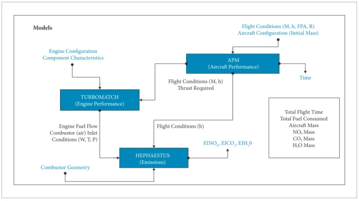
In the aircraft trajectory optimization processes, three computational models, i.e., aircraft performance simulation model (APM), engine performance simulation model (TurboMatch) and emissions prediction model (Hephaestus), have been utilized. Figure 1 illustrates the general arrangement of these models, as well as different parameters exchanged among them. The APM (Long, 2009) is a generic tool that determines flight path performance for a given aircraft design. It uses steady-state performance equations to resolve aerodynamic lift and drag and to determine the thrust required for a given kinematic flight state. In order to easily identify the behavior of Polyphemus, airspeed limitations – such as critical Mach number (M), never-exceed speed and wave drag at transonic M – have not been implemented in the model. As APM uses endpoints to compute performance, the user must declare a trajectory segment in terms of ground range and altitude intervals, whereby a constant flight path angle is then defined. Flight conditions are then assumed to be constant over that segment. The aircraft modeled in this work corresponds to a typical mid-sized, single-aisle, twin turbofan airliner with a maximum takeoff weight (MTOW) of about 72,000 kg and a seating capacity of about 150 passengers.
Figure 1. Computational models coniguration and exchange of parameters.
Models
Engine Configuration Component Characteristics
TURBOMATCH (Engine Performance)
Engine Fuel Flow Combustor (air) Inlet Conditions (W, T, P)
Combustor Geometry
HEPHAESTUS (Emissions)
EINOX, EICO2, EIH20
Flight Conditions (h) Flight Conditions (M, h)
Thrust Required
APM (Aircraft Performance)
Flight Conditions (M, h, FPA, R) Aircraft Configuration (Initial Mass)
Time
Total Flight Time Total Fuel Consumed
Aircraft Mass NO Mass CO Mass H O Mass
X
The performance of the engines was simulated using TurboMatch (Palmer, 1999), which is the in-house CU gas turbine performance code that has been developed and reined over a number of decades. TurboMatch performance simulations range from simple steady-state (design and of-design point) to complex transient performance computations. Finally, the gaseous emission predictions have been performed using the CU emissions prediction sotware, Hephaestus. An integral part of Hephaestus constitutes the emissions prediction model described in Celis et al. (2009), which follows an approach based on the use of a number of stirred reactors for modeling combustion chambers and estimating the level of pollutants emitted from them. Additional details of these computational models can be found in Celis et al. (2009) and Celis (2010).
Flight Proiles
It is clear that in order to demonstrate the suitability of an optimizer for optimizing aircrat trajectories, an extensive validation process of the algorithms that are implemented needs to be carried out using diferent analytical problems with known optimal values. In the case of Polyphemus, this part of the validation process has already been performed (Rogero, 2002) and is therefore not repeated here. In order to provide insight into the results that can be expected using Polyphemus, simpliied aircrat trajectory optimization processes using this optimizer have been performed. It is relevant to note that the main objective of these processes was evaluation of the mathematical performance of Polyphemus rather than the generation of realistic aircraft trajectories. Consequently, simplifications (in terms of number of light segments, design variables, constraints and objective functions, etc.) have been introduced when optimizing the aircrat light proiles. Indeed, the results discussed in this work correspond to single-objective optimization processes only, which means that the determination of non-dominated or Pareto optimal solutions that characterize multi-objective optimization processes is out of the scope of this work.
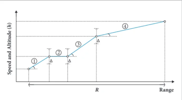
In this work, the aircrat light proiles have been divided into only a small number of segments, as illustrated in Fig. 2. his helps getting a greater visibility on the characteristics of the Polyphemus performance when assessing results. his would have been more diicult if the trajectory had been divided into a greater number of segments. hese hypotheses are a simpliication of real cases but provide numerical solutions that are used to commission the methodology. In order to obtain meaningful results in terms of actual optimum trajectories, the light path needs to be divided into a much larger number of segments, each small enough so
that the errors associated with the assumptions made within each segment will be cumulatively insigniicant. All the optimization processes carried out involved only vertical proiles. herefore, only three parameters have been used to deine a given aircrat trajectory: (1) light altitude (h); (2) aircrat speed: true airspeed (TAS), equivalent airspeed (EAS) or Mach number (M); and (3) range (R):the horizontal distance lown by the aircrat. One of the main uses of Polyphemus involves the optimization of aircrat trajectories between city pairs. hus, R has been usually kept constant during the optimizations, and only altitude and aircrat speed vary (i.e., used as design variables) to compute optimum aircrat trajectories that minimize, separately, total light time, fuel burned and NOx emissions.
Several aircraft flight profiles have been optimized in order to assess the mathematical performance of Polyphemus. he optimization results associated with three of these light proiles are summarized in this paper. A brief description of these proiles, which were analyzed as part of three separate case studies, is presented as follows:
• Case 1: Simple Climb Proile Optimization. (i) Flight proile has been divided into four segments (Fig. 2). (ii) Climb segments have been deined by arbitrary segment lengths (range, R). (iii) Overall climb has been deined by the cumulative range, start and end altitudes, and Mach numbers. (iv) Variation in intermediate Mach numbers (initial M in segments 2 and 3) and altitudes (initial altitude in segments 2, 3 and 4) has been allowed during the optimization processes. (v) Only explicit constraints have been utilized, i.e., range of permissible values of the design variables (h and M) are limited. (vi) Lower and upper bounds for these permissible ranges have been set at 457 m (1,500 t) and 10,668 m (35,000 t), respectively, for h (proile start and end altitudes); and 0.38 and 0.80, respectively, for M. (vii) International Standard Atmosphere
Figure 2. Generic aircraft light proile.
S
p
ee
d a
nd Al
ti
tu
d
e (
h
)
R Range
4
3 2
(ISA) conditions are assumed. (viii) Range of light path angle (FPA) allowed: [0, 7.5] deg. Data corresponding to this particular proile optimization are summarized in Table 1. • Case 2: Implicitly Constrained Climb Proile Optimization.
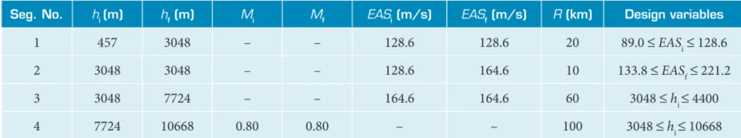
(i) Flight proile is similar to the proile used in Case 1; however, aircrat speeds have been speciied at the start and end of each climb segment allowing continuity in aircrat speed. (ii) Climb schedule has been described as follows; 1st seg.: climb at constant EAS from 1,500 t (457 m) up to 10,000 t (3,048 m); 2nd seg.: EAS acceleration at 10,000 t (level light); 3rd seg.: climb at constant EAS up to a segment inal altitude where (cruise) M is about 0.8; 4th seg.: climb at constant M from this altitude up to 35,000 t (10,668 m). (iii) Design variables and their range of permissible values: initial EAS in segment 1 (EAS1i [89.0, 128.6] m/s), inal EAS in segment 2 (EAS2f [133.8, 221.2] m/s), initial altitude in segment 3 (h3i [3048, 4400] m), and initial altitude in segment 4 (h4i [3048,10668] m). (iv) Implicit constraint: initial M in segment 4 (M4i)–allowable range ±0.5% of its nominal value, 0.8. (v) ISA conditions have been assumed. (vi) FPA range allowed: [0, 7.5] deg. Additional details about this case study are shown in Table 2.
• Case 3: Quasi-Full Flight Proile Optimization. (i) Flight proile (involving climb, cruise and descent) has been divided into eight segments. (ii) Proile has been deined following a similar approach to that used in Case 2. (iii) Flight schedule has been described as follows; 1st seg.: climb at constant EAS
from 1,500 t (457 m) up to 10,000 t (3,048 m); 2nd seg.: EAS acceleration at 10,000 t (level light); 3rd seg.: climb at constant EAS up to a segment inal altitude where (cruise) M
is about 0.8; 4th and 5th seg.: level light cruise at constant
M; 6th seg.: descent at constant EAS to 10,000 t (3,048 m); 7th seg.: EAS deceleration at 10,000 t (level light); and 8th seg.: descent at constant EAS from 10,000 t (3,048 m) to 1,500 t (457 m). (iv) Design variables and their range of permissible values: initial EAS in segment 1 (EAS1i [89.0, 128.6] m/s), inal EAS in segment 2 (EAS2f [117.1, 184.6] m/s), initial altitude in segment 3 (h3i [3048, 4400] m), initial altitude in segment 4 (h4i [6096, 12192] m), initial altitude in segment 7 (h7i [3048, 4400] m), and initial EAS in segment 8 (EAS8i [89.0, 128.6] m/s). (v) Implicit constraint: initial M
in segment 4 (M4i)–allowable range ±0.5% of its nominal value, 0.8. (vi) ISA conditions have been assumed. (vii) FPA range allowed: [0, 7.5] deg during climb and cruise, and [-7.5, 0] deg during descent. Table 3 summarizes the data associated with this light proile optimization.
he lower and upper bounds of the range of permissible values of the design variables were in general deined in a way to reduce the computational time of the optimization processes, to take into account typical air traic control (ATC) restrictions, and/or to avoid the aircrat losing (gaining) altitude during climb (descent) processes. For instance, below 10,000 t, the EAS lower and upper bounds usually correspond to, respectively, the aircrat stall speed (89.0 m/s
Table 1. Case 1 (simple climb proile) – Baseline trajectory and design variables.
Seg. No. hi(m) hf(m) M R (km) Design variables
1 457 3048 0.38 20 –
2 3048 3048 0.46 10 0.38 ≤Mi≤ 0.80; 457 ≤hi≤ 10668
3 3048 7000 0.58 60 0.38 ≤Mi≤ 0.80; 457 ≤hi≤ 10668
4 7000 10668 0.80 100 457 ≤hi≤ 10668
Table 2. Case 2 (implicitly constrained climb proile) – Baseline trajectory and design variables.
Seg. No. hi (m) hf(m) Mi Mf EASi (m/s) EASf (m/s) R (km) Design variables
1 457 3048 – – 128.6 128.6 20 89.0 ≤EASi≤ 128.6
2 3048 3048 – – 128.6 164.6 10 133.8 ≤EASf≤ 221.2
3 3048 7724 – – 164.6 164.6 60 3048 ≤hi ≤ 4400
EAS for the particular aircra odeled) and the maximum EAS
permissible below this altitude (according to ATC restrictions), i.e., 250 kts EAS or 128.6 m/s. In Case 3, in particular, the range of values in which the initial altitude in segment 4 can vary was established in a way to allow the aircrat cruising at altitudes between 20,000 t (6,096 m) and 40,000 t (12,192 m). hus, EAS2f permissible values were limited to those speeds that yield Mach numbers of about 0.8 at these cruise altitudes. Similar considerations were made in the other case studies analyzed in this work.
Optimization Process
According to the methodology followed in this work for optimizing a given aircrat trajectory, Polyphemus irst randomly changes the values of the design variables (altitude and/or aircrat speed in one or more trajectory segments) in order to create a group of potential solutions. For a given potential solution, by making use of the initial aircrat weight (aircrat empty weight plus fuel on-board, constant), the APM carries out the computations related to the irst segment of the aircrat trajectory, and determines the thrust required, light time, etc. (Fig. 1). TurboMatch subsequently uses the light conditions and the thrust required to determine the engine operating point, thereby establishing the engine fuel low and the combustor inlet conditions among others. Hephaestus then makes use of the combustor inlet conditions and combustor geometric parameters to calculate the emission indices for the main pollutants. Based on the fuel low and light time, the fuel burned during the irst trajectory segment and the new aircrat weight (i.e. the initial weight less fuel burned) are calculated. Computations continue in a similar fashion for all the remaining trajectory segments. When all the segments have been computed, among other calculations, the total light time, fuel burned and gaseous
emissions produced during the whole aircrat trajectory are also computed. his process is repeated for all the potential solutions, and for all generations of potential solutions that Polyphemus utilizes in order to determine an optimum trajectory according to given criteria initially speciied by the designer. he results were obtained following a procedure similar to that described before.
RESULTS AND DISCUSSIONS
Main results of the optimization processes corresponding to three case studies indicated above are summarized in this section. In these processes, the minimization of total light time, fuel burned, and NOX emissions have been considered as the objective functions.
Case 1: Simple Climb Proile Optimization
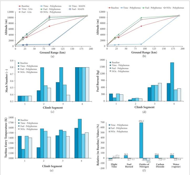
he baseline climb proile for this case study as well as the optimum trajectories computed using Polyphemus and two commercial optimizers (MATLAB
®
, 2008) are illustrated in Fig. 3. Two diferent approaches used within the commercial package were (i) a pattern search algorithm called mesh adaptive search (MADS), and (ii) GAs. Both Polyphemus and the commercial optimizers yielded very similar results (Fig. 3a). Even though this irst optimization case study (climb proile) corresponded to a hypothetical one, the reasonable agreement among the optimizers (average discrepancies ~2%) conirmed the validity of the approach. Figure 3c shows that in order to minimize the time spent during climb, Polyphemus suggests a solution where the aircrat lies at the highest M permissible, which was ixed at 0.38 and 0.80 in the irst and fourth segment, respectively, and free to rise to 0.8 in the remaining middle two. Polyphemus alsoTable 3. Case 3 (quasi-full light proile) – Baseline trajectory and design variables.
Seg. No. hi (m) hf (m) Mi Mf EASi (m/s) EASf (m/s) R (km) Design variables
1 457 3048 – – 128.6 128.6 20 89.0 ≤EASi≤ 128.6
2 3048 3048 – – 128.6 164.6 10 117.1 ≤EASf≤ 184.6
3 3048 7724 – – 164.6 164.6 160 3048 ≤hi ≤ 4400
4 7724 7724 0.80 0.80 – – 230 6096 ≤hi ≤ 12192
5 7724 7724 0.80 0.80 – – 230 –
6 7724 3048 – – 164.6 164.6 140 –
7 3048 3048 – – 164.6 128.6 20 3048 ≤hi ≤ 4400
suggests that the aircra should ly at low altitudes for as long as possible
before climbing rapidly to the target end altitude (Fig. 3b). his is mathematically correct because the speed of sound is the highest at sea level, thus enabling the aircrat to ly faster (maximization of TAS) if it could actually achieve M 0.8 at this level. his solution, however, does not represent practical light proiles because never exceed speed (VNE) is much lower than M 0.8 at sea level, thus restricting large transport category aircrat from approaching such high Mach numbers. Nevertheless, it is an interesting solution, conirming that the optimizer is working correctly in the absence of M (or TAS) constraints.
Figure 3 also illustrates that in order to reduce fuel burn, the optimizer suggests lying slower (Fig. 3c) and higher (Fig. 3b) than the reference trajectory (segment 3). his is again conceptually correct given the current reference trajectory. It is interesting to note that the fuel optimized trajectory proposes second and third segments afording a greater fuel burn (relative to the baseline) (Fig. 3d) in order to gain height (Fig. 3b), which then subsequently yields a lower fuel burn in the last segment and an overall lower fuel burn for the climb proile as a whole. In terms of light proile, one could conclude from Fig. 3b that the trajectories optimized for minimum fuel burned and NOX emissions are similar. However,
Baseline
200
Time - Polyphemus Time - MADS
12000 Al ti tu d e (m )
Time - GAs Fuel - GAs
Fuel - Polyphemus Fuel - MADS
NOx - Polyphemus
10000 8000 6000 4000 2000 0
Ground Range (km)
175 150 125 100 75 50 25 0 Baseline 200 Time - Polyphemus
12000 Al ti tu d e (m)
Fuel - Polyphemus NOx - Polyphemus
10000 8000 6000 4000 2000 0
Ground Range (km)
175 150 125 100 75 50 25 0 Baseline Time - Polyphemus 0.9 M ac h N um b e r
(--) Fuel - Polyphemus
NOx - Polyphemus 0.8 0.7 0.6 0.5 0.4 0.3
Climb Segment
4 3
2 1
Baseline Time - Polyphemus 1800 F u e l B urne d (kg)
Fuel - Polyphemus NOx - Polyphemus 1500 1200 900 600 300 0 Climb Segment 4 3 2 1 Baseline Time - Polyphemus 1800 T urb ine E n tr y T em p er at ur e (K)
Fuel - Polyphemus NOx - Polyphemus 1700 1600 1500 1400 1300 1200 Climb Segment 4 3 2 1 1100 1000 694.2 Time - Polyphemus
700 R el at iv e (t o Bas eline) V al u
es (%) Fuel - PolyphemusNOx - Polyphemus 600 500 400 300 200 100 0 -100 -200 17.1 3.7 -16.2 -1.1 50.5 -6.7 -1.3 55.6 -7.0 -1.4 55.7 -6.9 -43.6 -19.3 Carbon Dioxide Oxides of Nitrogen Fuel Burned Flight
Time (vapour)Water
(a) (c) (e) (b) (d) (f)
there are signant diferences between these two trajectories.
The main diference is related to the fact that the NOX emissions optimized trajectory is lown at relatively lower Mach numbers than the fuel burned optimized trajectory (Fig. 3c). hese lower Mach numbers result in lower engine thrust settings, i.e., the thrust required to ly a given segment is lower, which in turn results in lower engine turbine entry temperature (TET) values (Fig. 3e). Consequently, as one of the main factors determining the level of NOX emissions produced (besides the fuel burned) is TET, the trajectory optimized for minimum NOX emissions produces a signiicant reduction in the amount of NOX emitted (~-43%). Interestingly, Fig. 3e shows that in order to minimize NOX emissions, the optimizer proposes a trajectory in which the engine TET remains almost constant (~1,400–1,500 K) for the entire climb proile. It is relevant to note in this discussion that the level of NOX formed at temperatures near to and above 1,700–1,800 K increases exponentially with temperature.
An aspect to be highlighted in Fig. 3f is the level of gaseous emissions (NOX, CO2 and H2O) associated with the optimum trajectories relative to the reference climb trajectory. As expected, variations in CO2 and H2O are directly proportional to the variations in the amount of fuel burned (species in chemical equilibrium). However, the aircrat trajectory optimized for total light time significantly increases the amount of NOX emissions. One of the main factors responsible for this signiicant increase in NOX emissions (besides the increase in fuel burn) is the increase in TET resulting from the higher thrust settings. Fig. 3f also illustrates the increase in total light time associated with the trajectory optimized for minimum NOX emissions. Although this parameter increases, the total fuel burned slightly decreases as a consequence of the lower thrust settings (i.e., lower engine fuel low relative to the baseline trajectory). Additional details about the results analyzed in this irst case study can be found in Celis et al.(2009). In the following two case studies, complexities (in terms of operational constraints, number of segments, number of trajectory light phases, etc.) were included gradually. his gradual approach aforded greater visibility of the mathematical performance of Polyphemus when assessing results, which would have been more diicult if the analysis had been initiated with very complex trajectories.
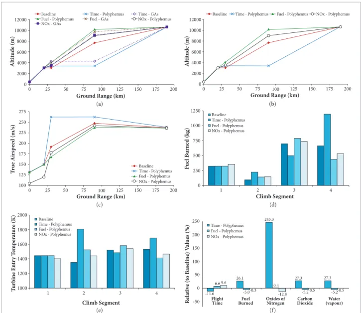
Case 2: Implicitly Constrained Climb Proile Optimization
Results obtained in the second case study (Fig. 4) are in general similar to those obtained in the irst case study. hus, when minimizing the time spent during climb, i.e., maximizing
TAS, Polyphemus suggests a solution where the aircrat lies the irst segment at the highest EAS permissible (ixed at 128.6 m/s) (Fig. 4c). his is conceptually correct because in the irst segment, since the light altitude is ixed, TAS increases with the increase in EAS. The optimizer also suggests that the aircraft should accelerate in the second segment to the highest EAS permissible (ixed at 221.2 m/s), and ly the following segments at low levels (Fig. 4b) as long as possible before climbing rapidly to the target end altitude. his is again mathematically correct because, irstly, as previously indicated, once the light altitude has been established, the TAS increases with increase in EAS; and, secondly, for a given M, TAS increases with the decrease in altitude (speed of sound is the highest at sea level). Clearly, the inluence of the third and fourth segments on the total climb time is more important than the corresponding second segment. Otherwise, the initial altitude in segment 3 would be the highest permissible.
Baseline
200 Time - Polyphemus
12000 Al ti tu d e (m)
Time - GAs Fuel - GAs
Fuel - Polyphemus NOx - Polyphemus
10000 8000 6000 4000 2000 0
Ground Range (km)
175 150 125 100 75 50 25 0
NOx - GAs
Baseline
200 Time - Polyphemus
12000 Al ti tu d e (m)
Fuel - Polyphemus NOx - Polyphemus
10000 8000 6000 4000 2000 0
Ground Range (km)
175 150 125 100 75 50 25 0 Baseline Time - Polyphemus
T r u e A irs p ee d (m/s)
Fuel - Polyphemus NOx - Polyphemus
200
Ground Range (km)
175 150 125 100 75 50 25 0 200 175 150 125 100 225 250 275 Baseline Time - Polyphemus 1250 F u e l B urne d (kg)
Fuel - Polyphemus NOx - Polyphemus 1000 750 500 250 0 Climb Segment 4 3 2 1 Baseline Time - Polyphemus 1800 T urb ine E n tr y T em p er at ur e (K)
Fuel - Polyphemus NOx - Polyphemus 2000 1600 1400 1200 Climb Segment 4 3 2 1 1000 245.3 Time - Polyphemus
R el at iv e (t o Bas eline) V al u es (%)
Fuel - Polyphemus NOx - Polyphemus 250 200 150 100 50 0 -50 9.6 6.6 -11.6 -0.3 26.1 -5.0 -0.5 27.3 -5.2 -0.5 27.3 -5.2 -12.8 0.4 Carbon Dioxide Oxides of Nitrogen Fuel Burned Flight
Time (vapour)Water
Figure 4. Case 2 – Implicitly constrained climb proile optimisation results.
(a) (c) (e) (b) (d) (f)
negatively afects the fuel burned during the process. herefore, a compromise between aircrat light altitude and speed, which directly affect the changes in the aircraft mass, needs to be achieved at some stage. he fuel-optimized trajectory computed is a typical example of the referred compromise. It is interesting to note in Fig. 4d that this fuel-optimized trajectory proposes second and third segments afording a greater fuel burn (relative to the baseline) in order to gain height (Fig. 4b), which, then, is translated into a lower fuel burn in the last segment and an overall lower fuel burn for the whole climb proile.
Regarding the trajectory optimized for minimum NOX emissions, the results show that, similar to the fuel optimized one, this trajectory
utilized, the total amount of fuel burned is slightly reduced. In Fig. 4f, it should also be noticed that the aircrat trajectory optimized for minimum light time signiicantly increases the amount of NOX emissions. his is partially because of the large amount of thrust required to increase both aircrat kinetic energy in segment 2 and potential energy in segment 4. his higher engine thrust requirement is translated into higher TET values (Fig. 4e), and consequently into a signiicant increase in the level of NOX emissions.
Case 3: Quasi-Full Flight Proile Optimization
As highlighted before and illustrated in Fig. 5, which shows the main results obtained for this particular case study, minimization of total flight time implies maximization of TAS (Fig. 5c).
hus, when determining the minimum light time-optimized trajectory, Polyphemus suggests a solution in this case, where the aircrat lies the irst and the last segments at the highest EAS permissible (ixed at 128.6 m/s). his is conceptually correct because the irst and last segments are lown at ixed altitudes, where TAS increases with the increase in EAS. Polyphemus also suggests that the aircrat should accelerate in the second segment to the highest EAS permissible (ixed at 184.6 m/s), and start the third segment as high as possible, and the fourth one as low as possible. his is again mathematically correct because, irstly, TAS increases with the increase in both light altitude and EAS (segments 2 and 3); and, secondly, for a given Mach number, the TAS increases with the decrease in altitude (segments 4 and 5).
Baseline
800 Time - Polyphemus
12000 Al ti tu d e (m)
Time - GAs Fuel - GAs
Fuel - Polyphemus NOx - Polyphemus
10000 8000 6000 4000 2000 0
Ground Range (km)
700 600 500 400 300 200 100 0
NOx - GAs
900
Baseline
800 Time - Polyphemus
12000 Al ti tu d e (m)
Fuel - Polyphemus NOx - Polyphemus
10000 8000 6000 4000 2000 0
Ground Range (km)
700 600 500 400 300 200 100 0 900 Baseline Time - Polyphemus
T ru e A irs p ee d (m/s)
Fuel - Polyphemus NOx - Polyphemus
Ground Range (km) 195 155 115 75 235 275 800 700 600 500 400 300 200 100 0 900 Baseline Time - Polyphemus 1500 F u e l B urne d (kg)
Fuel - Polyphemus NOx - Polyphemus 1200
900
600
300
0
Flight Segment4
3 2
1 5 6 7 8
Baseline Time - Polyphemus 1800 T urb ine E n tr y T em p er at ur e (K)
Fuel - Polyphemus NOx - Polyphemus 2000 1600 1400 1200 1000 800 Flight Segment 4 3 2
1 5 6 7 8
126.7 Time - Polyphemus
R el at iv e (t o Bas eline) V al u
es (%) Fuel - PolyphemusNOx - Polyphemus
75 125 150 100 25 Carbon Dioxide Oxides of Nitrogen Fuel Burned Flight Time 0 -50 9.8 8.8 -5.2 -13.3 14.5 -17.2 -13.5 14.7 -17.4 -35.1 -24.7 -25 50 -13.5 14.7 -17.4 Water (vapour) (a) (c) (e) (b) (d) (f)
As a consequence of the larger distance covered by the cruise segments 4 and 5 , their inluence on the total light time is more important than that associated with the third and sixth segments. his is emphasized by the fact that the aircrat has a tendency to cruise at low altitude levels as observed in Fig. 5b.
Regarding the fuel-optimised trajectory, it is observed that in order to reduce the total fuel burned, the optimiser suggests flying mostly slower (Fig. 5c) and higher (Fig. 5b) than the reference trajectory. In particular, it suggests lying the irst segment at the highest EAS permissible. his situation is similar to that encountered in the second case study. In order to minimize the total fuel burned during the light proile, the total energy required during the process must be minimized. In this case, it implies, in turn, minimization of the aircrat kinetic energy change; or, more speciically, maximization of the initial aircrat speed and minimization of the inal one (in terms of TAS). As in the second case study, this TAS maximization makes the aircrat ly the irst segment at the highest EAS permissible. Results also show that even though the aircrat arrives to the endpoint at a low speed, this does not correspond to the lowest EAS permissible (ixed at 89.0 m/s), as it could be expected. It is believed that one aspect that might be inluencing this particular result is the path-dependent energy, which has a direct relationship with the aircrat speed and also needs to be minimum. In the foregoing analysis, the aircrat mass changes were not considered. hese mass changes cannot be ignored however because in reality they are one of the main factors driving the minimization of the fuel burned during the optimization process. As highlighted before, there are two main parameters that afect the fuel burned and, consequently, the changes in the aircrat mass: the aircrat speed and the aircrat light altitude. hese two parameters directly or indirectly afect, in turn, other parameters, such as drag, thrust required, light time and engine thrust setting (consequently, fuel low, TET, etc.), among others. It implies that a fuel-optimized trajectory represents in fact a tradeof among all these parameters, some of which conlict with each other.
he light proile optimized for minimum NOx emissions is lown similar to the fuel-optimized one, i.e., mostly slower (Fig. 5c) and higher (Fig. 5b) than the baseline trajectory utilized. In general, the relative lower speed and higher altitude utilized to ly this trajectory lead to a reduction in the thrust required to ly the trajectory segments. hese lower thrust requirements are in turn translated into lower engine TET values (Fig. 5), which ultimately result in a reduction in the level of NOX emissions produced (Fig. 5f). Fig. 5e shows, in particular, that from all TET
values, those corresponding to the NOX emissions, optimised trajectory values are the lowest ones. his is expected, of course, because this parameter has a direct inluence on the level of NOX emissions produced. In Fig. 5f, it can also be observed that the changes in CO2 and H2O present the expected behavior, and, even though the NOX emissions optimized trajectory increases the total light time, the total amount of fuel burned is largely reduced. his is a consequence of the lower engine thrust settings utilized to ly this trajectory. As in the irst two case studies, the aircraft trajectory optimized for minimum flight time signiicantly increases the amount of NOx emissions (Fig. 5f). his is partially due to the large amount of thrust required to ly some of the segments of this particular optimized trajectory.
CONCLUSIONS
REFERENCES
Betts, J., 1998, “Survey of Numerical Methods for Trajectory Optimization”, Journal of Guidance, Control, and Dynamics, Vol. 21, No. 2, pp. 193–207.
Boeing Commercial Airplanes, “Market Analysis, Boeing Current Market Outlook 2009 to 2028”, Available from: www.boeing.com/cmo. Accessed on: 16 August 2009.
Brooker, P., 2006, “Civil Aircraft Design Priorities: Air Quality? Climate Change? Noise?”, The Aeronautical Journal, Vol. 110, No. 1110, pp. 517–532.
Bunday, B.D., 1984, “Basic Optimisation Methods”, Edward Arnold, London, UK.
Callan, R., 2003, “Artiicial Intelligence”, Palgrave Macmillan, New York, US.
Celis, C., 2010, “Evaluation and Optimisation of Environmentally Friendly Aircraft Propulsion Systems”, Ph.D. Thesis, School of Engineering, Cranield University.
Celis, C., Long, R., Sethi, V. and Zammit-Mangion, D., 2009, “On Trajectory Optimisation for Reducing the Impact of Commercial Aircraft Operations on the Environment”, 19th Conference of the International Society for Air Breathing Engines, ISABE-2009, Montréal, Canada.
Celis, C., Moss, B. and Pilidis, P., 2009, “Emissions Modelling for the Optimisation of Greener Aircraft Operations”, Proceedings of GT2009, ASME Turbo Expo 2009, Power for Land, Sea and Air, Orlando, Florida, USA.
Clarke, J.P., 2003, “The Role of Advanced Air Trafic Management in Reducing the Impact of Aircraft Noise and Enabling Aviation Growth”, Journal of Air Transport Management, Vol. 9, No. 3, pp. 161–165.
Clean Sky JTI (Joint Technology Initiative), 2009, Available from: www. cleansky.eu. Accessed on: 18 August 2009.
Davis, L. (editor), 1991, “Handbook of Genetic Algorithms”, Van Nostrand Reinhold, New York, US.
Everitt, B., 1987, “Introduction to Optimization Methods and their Application in Statistics”, Chapman and Hall, London, UK.
Fletcher, R., 1987, “Practical Methods of Optimization”, 2nd Edition, John Wiley, Chichester, UK.
Goldberg, D.E., 1989, “Genetic Algorithms in Search, Optimization and Machine Learning”, Addison-Wesley, Reading, MA, US.
Green, J. E., 2003, “Civil Aviation and the Environmental Challenge”, The Aeronautical Journal, Vol. 107, No. 1072, pp. 281–299.
Gulati, A., 2001, “An Optimization Tool for Gas Turbine Engine Diagnostics”, Ph.D. Thesis, School of Engineering, Cranield University.
Hartley, S.J., 1998, “Concurrent Programming: The Java Programming Language”, Oxford University Press, New York, US.
Krotov, V.F., 1996, “Global Methods in Optimal Control Theory”, Marcel Dekker, New York, US.
Long, R.F., 2009, “An Aircraft Performance Model for Trajectory Optimisation”, School of Engineering, Cranield University, UK (unpublished).
MATLAB®, 2008, “The Language of Technical Computing, Version 7.7
(R2008b)”, The MathWorks, Inc. Available from: www.mathworks.com.
Palmer, J.R., 1999, “The TurboMatch Scheme for Gas-Turbine Performance Calculations, User’s Guide”, Cranield University, Cranield, UK.
PARTNER, 2009, “Partnership for AiR Transportation Noise and Emissions Reduction”, Available from: web.mit.edu/aeroastro/ partner/. Accessed on: 18 August 2009.
Quagliarella, D., 1998, “Genetic Algorithms and Evolution Strategy in Engineering and Computer Science, Recent Advances and Industrial Applications”, John Wiley & Sons, Ltd., Chichester, UK.
Rao, S.S., 1996, “Engineering Optimization: Theory and Practice”, 3rd Edition, John Wiley, New York, US.
Riddlebaugh, S.M. (editor), 2007, “Research & Technology 2006, NASA/TM – 2007-214479”, NASA Glenn Research Center, Cleveland, Ohio, USA.
Rogero, J.M., 2002, “A Genetic Algorithms-based Optimisation Tool for the Preliminary Design of Gas Turbine Combustors”, Ph.D. Thesis, School of Mechanical Engineering, Cranield University.
Rogero, J.M. and Rubini, P.A., 2003, “Optimisation of Combustor Wall Heat Transfer and Pollutant Emissions for Preliminary Design Using Evolutionary Techniques”, Proceedings of the Institution of Mechanical Engineers, Part A: Journal of Power and Energy, Vol. 217, No. 6,pp. 605–614.
Russell, S. and Norvig, P., 2003, “Artiicial Intelligence: A Modern Approach”, 2nd Edition, Prentice Hall, New Jersey, US.
Sampath, S., 2003, “Fault Diagnostics for Advanced Cycle Marine Gas Turbine Using Genetic Algorithms”, Ph.D. Thesis, School of Engineering, Cranield University.
Schwefel, H.P., 1981, “Numerical Optimization of Computer Models”, John Wiley, Chichester, UK.
Walsh, G.R., 1975, “Methods of Optimization”, John Wiley, London, UK.
Wienke, D., Lucasius, C.B. and Kateman, G., 1992, “Multicriteria Target Vector Optimization of Analytical Procedures Using a Genetic Algorithm. Part I. Theory, Numerical Simulation and Application to Atomic Emission Spectroscopy”, Analytica Chimica Acta, Vol. 265, No. 2, pp. 211–225.
ACKNOWLEDGMENTS
During this work, Cesar Celis was partially supported by the Programme Alβan, the European Union Programme of High Level Scholarships for Latin America, Scholarship No. E07D400097BR. Source of inancing: European Union.