Optimizing global CO emissions using a four-dimensional variational data assimilation system and surface network observations

(1)

ACPD

11, 341–386, 2011

Optimizing CO emissions in a 4D-VAR framework

P. B. Hooghiemstra et al.

Title Page

Abstract Introduction

Conclusions References

Tables Figures

◭ ◮

Back Close

Full Screen / Esc

Printer-friendly Version Interactive Discussion

Discussion

P

a

per

|

Dis

cussion

P

a

per

|

Discussion

P

a

per

|

Discussio

n

P

a

per

|

Atmos. Chem. Phys. Discuss., 11, 341–386, 2011 www.atmos-chem-phys-discuss.net/11/341/2011/ doi:10.5194/acpd-11-341-2011

Atmospheric Chemistry and Physics Discussions

This discussion paper is/has been under review for the journal Atmospheric Chemistry and Physics (ACP). Please refer to the corresponding final paper in ACP if available.

Optimizing global CO emissions using

a four-dimensional variational data

assimilation system and surface network

observations

P. B. Hooghiemstra1,2, M. C. Krol1,2,3, J. F. Meirink4, P. Bergamaschi5, G. R. van der Werf6, P. C. Novelli7, I. Aben2,6, and T. R ¨ockmann1

1

Institute for Marine and Atmospheric Research Utrecht, University of Utrecht, Utrecht, The Netherlands

2

Netherlands Institute for Space Research (SRON), Utrecht, The Netherlands

3

Wageningen University and Research Centre, Wageningen, The Netherlands

4

Royal Netherlands Meteorological Institute (KNMI), de Bilt, The Netherlands

5

European Commission Joint Research Centre, Institute for Environment and Sustainability, Ispra, Italy

6

Faculty of Earth and Life Sciences, VU University, Amsterdam, The Netherlands

7

(2)

ACPD

11, 341–386, 2011

Title Page

Tables Figures

◭ ◮

Back Close

Full Screen / Esc

Discussion

P

a

per

|

Dis

cussion

P

a

per

|

Discussion

P

a

per

|

Discussio

n

P

a

per

|

Received: 8 October 2010 – Accepted: 13 December 2010 – Published: 6 January 2011

(3)

ACPD

11, 341–386, 2011

Title Page

Tables Figures

◭ ◮

Back Close

Full Screen / Esc

Discussion

P

a

per

|

Dis

cussion

P

a

per

|

Discussion

P

a

per

|

Discussio

n

P

a

per

|

Abstract

We apply a four-dimensional variational (4D-VAR) data assimilation system to optimize carbon monoxide (CO) emissions for 2003 and 2004 and to reduce the uncertainty of emission estimates from individual sources using the chemistry transport model TM5. The system is designed to assimilate large (satellite) datasets, but in the current study

5

only a limited amount of surface network observations from the National Oceanic and Atmospheric Administration Earth System Research Laboratory (NOAA/ESRL) Global Monitoring Division (GMD) is used to test the 4D-VAR system. By design, the system is capable to adjust the emissions in such a way that the posterior simulation reproduces background CO mixing ratios and large-scale pollution events at background stations.

10

Uncertainty reduction up to 60% in yearly emissions is observed over well-constrained regions and the inferred emissions compare well with recent studies. However, with the limited amount of data from the surface network, the system becomes data sparse. This results in a large solution space and the 4D-VAR system has di_fficulties in sep-arating anthropogenic and biogenic sources in particular. In addition we show that

15

uncertainties in the model such as biomass burning injection height and the OH distri-bution largely influence the inversion results. The inferred emissions are validated with NOAA aircraft data over North America and the agreement is significantly improved from prior to posterior simulation. Validation with the Measurements Of Pollution In The Troposphere (MOPITT) instrument version 4 (V4) shows only a slight improved

20

(4)

ACPD

11, 341–386, 2011

Title Page

Tables Figures

◭ ◮

Back Close

Full Screen / Esc

Discussion

P

a

per

|

Dis

cussion

P

a

per

|

Discussion

P

a

per

|

Discussio

n

P

a

per

|

1 Introduction

Understanding the budget of carbon monoxide (CO) is important, because by reaction with the radical OH, CO influences the oxidizing capacity of the atmosphere signifi-cantly (Logan et al., 1981). Enhanced CO concentrations reduce OH concentrations and this has a feedback on the concentration of methane, the second most important

5

anthropogenic greenhouse gas. CO is also a precursor of tropospheric ozone un-der high NO_x (NO₊NO₂) conditions (Seinfeld and Pandis, 2006). CO is emitted into the atmosphere by incomplete combustion of fossil fuels, biofuels and during biomass burning events. In addition, CO is produced throughout the atmosphere by oxidation of methane and non-methane volatile organic compounds (NMVOCs). The main sink

10

of CO is the reaction with the OH radical, the so-called cleansing agent of the atmo-sphere (Logan et al., 1981). Deposition of CO on the Earth’s surface is a minor sink, accounting for 5–10% of the total sink strength (Sanhueza et al., 1998; P ´etron et al., 2002).

The magnitude of CO emissions from different source categories is not well

quan-15

tified. In particular, emissions from biomass burning (most importantly forest and sa-vanna fires) carry large uncertainties partly due to the variability of fires in both space and time. In addition, bottom-up inventories like the widely used Global Fire Emission Database (GFED) (van der Werf et al., 2004, 2006, 2010) come with substantial un-certainties due to insufficient knowledge about burned area, fuel load, and emission

20

factors (van der Werf et al., 2006). Uncertainties in biomass burning emission esti-mates are largest in deforestation regions (e.g., South America and Indonesia) and regions where organic soils burn (e.g., Indonesia and the Boreal region).

One way to better constrain emissions of CO is inverse modeling (Enting, 2002). In short, atmospheric measurements, a chemistry transport model (CTM) and a priori

25

(5)

lit-ACPD

11, 341–386, 2011

Title Page

Tables Figures

◭ ◮

Back Close

Full Screen / Esc

Discussion

P

a

per

|

Dis

cussion

P

a

per

|

Discussion

P

a

per

|

Discussio

n

P

a

per

|

erature there are basically two inversion methods used for CO inversions: Synthesis Bayesian inversions (e.g., Bergamaschi et al., 2000; Kasibhatla et al., 2002; P étron et al., 2002; Palmer et al., 2003, 2006; Arellano et al., 2004, 2006; Heald et al., 2004; Jones et al., 2009) and adjoint inversions (e.g., M üller and Stavrakou, 2005; Yumimoto and Uno, 2006; Stavrakou and M üller, 2006; Chevallier et al., 2009; Kopacz et al., 2009,

5

2010; Fortems-Cheiney et al., 2009; Tangborn et al., 2009). The synthesis inversion optimizes CO emissions over large geographical regions with a preset CO emission distribution in each region, whereas the adjoint inversion technique is capable to derive optimized CO emissions on the grid-scale of the underlying CTM, thereby reducing the risk of aggregation errors (Kaminski et al., 2001). An iterative approach is used to

10

minimize the mismatch between model and observations. Adjoint inversions are in par-ticular suited for assimilation of large observational (satellite) datasets (Bergamaschi et al., 2009; Meirink et al., 2008b).

In the current study we apply a 4D-VAR system for CO based on the earlier work for methane (Meirink et al., 2008a,b; Bergamaschi et al., 2009). Although this system is

15

designed to assimilate large amounts of observational data, it will be tested in this first study by only assimilating surface observations from a limited number of NOAA stations to optimize monthly mean CO emissions for a period of two years. This approach is followed to obtain a benchmark characterization of the system for future assimilation of satellite data. Firstly, we focus on the capability of the system to estimate annual

20

continental emissions by inspecting the reduction of the prior errors that are set on the sources. The optimized emissions will be validated by comparing model results to independent aircraft data from NOAA and satellite data from the Measurements Of Pollution in The Troposphere (MOPITT) instrument (Deeter et al., 2003, 2007, 2010). Secondly, we will investigate the influence of prior settings and model errors on the

25

inversion results by performing sensitivity studies.

(6)

ACPD

11, 341–386, 2011

Title Page

Tables Figures

◭ ◮

Back Close

Full Screen / Esc

Discussion

P

a

per

|

Dis

cussion

P

a

per

|

Discussion

P

a

per

|

Discussio

n

P

a

per

|

results are discussed in Sect. 4 and the performance of the 4D-VAR system is further investigated by performing sensitivity studies (Sect. 5). Finally we give conclusions in Sect. 6.

2 Description of the four dimensional variational data assimilation system

The 4D-VAR modeling system for CO is based on the TM5-4DVAR system originally

5

developed for methane (Meirink et al., 2008b; Bergamaschi et al., 2009). Given a set of atmospheric observations y and a chemistry transport model H it is possible to

optimize a set of fluxesx (the state vector) using the Bayesian technique (Rodgers,

2000). The a posteriori vector x is found by minimizing the mismatch between the

model forward simulationH(x) and the observations (y) weighted by an observation

10

error covariance matrixR while staying close to a set of a priori fluxes x_b, weighted

with the a priori error covariance matrixB. Mathematically this problem can be written as the following minimization problem:

ˆ

x=ArgminJ (1)

J(x)=1

2(x−xb)

T

B−1(x−x_b)+1

2 n X

i=1

(Hi(x)−yi)TR

−1

i (Hi(x)−yi), (2)

15

where the indexi refers to the time step and T is the transpose operator. Observations

y_i are assimilated in the 4D-VAR system at time i. The classic Bayesian approach

determines the a posteriori solutionxˆ (Rodgers, 2000):

ˆ

x=x_b+K(Hx−y), (3)

withK=BHT HBHT+R−1

and His the Jacobian matrix corresponding to the CTMH

20

(Arellano et al., 2004). The a posteriori error covariance matrixAcan be written as

A₌ HTR−1H₊B−1−1

(7)

ACPD

11, 341–386, 2011

Title Page

Tables Figures

◭ ◮

Back Close

Full Screen / Esc

Discussion

P

a

per

|

Dis

cussion

P

a

per

|

Discussion

P

a

per

|

Discussio

n

P

a

per

|

When the number of state vector variables is large, it is not possible to compute the inverse matrices in the above equations directly. Hence an iterative minimization al-gorithm is required. The conjugate gradient method (Fisher, 1998) can be used to minimize the cost function (2) if the CTM is linear. In general, the CTMH is nonlinear with respect to the state vectorxsince the CO emissions perturb OH concentrations

5

and hence the CO sink term. However, for tropospheric CO, P ´etron et al. (2002) have shown that to a reasonable approximation, the system can be linearized by using fixed OH fields. In this case the cost function J is quadratic and can be minimized using the conjugate gradient method (Fisher, 1998). This method is a generalization of the steepest descend method that also yields the leading eigenvaluesλ_i and eigenvectors

10

νi of the Hessian of the cost function. The a posteriori error covariance matrix (Eq. 4) describing the uncertainty in the optimized state vectorxˆ, equals the inverse Hessian

of the cost function. Hence, the a posteriori error covariance matrix is approximated by a finite combination of the leading eigenvalues and eigenvectors of the Hessian of the cost function added by the a priori error covariance matrixB(Fisher and Courtier,

15

1995):

A≈B₊

N X

i=1

1

λi

−1

(Lνi)(Lνi)T, (5)

whereLis the preconditioner explained below.

The rate of convergence of the minimization is in general quite slow, but a precondi-tioner can be used to speed up the convergence rate. Fisher and Courtier (1995) have

20

shown that the matrixLsuch thatLLT₌Bis a suitable preconditioner when used in this 4D-VAR approach. However, due to the large number of state vector elements, it is not possible to store this preconditioner in this form in memory. We will follow the approach of Meirink et al. (2008b) to store the preconditionerL. In our study, we consider the method converged when the norm of the gradient of the cost function is reduced by

25

(8)

ACPD

11, 341–386, 2011

Title Page

Tables Figures

◭ ◮

Back Close

Full Screen / Esc

Discussion

P

a

per

|

Dis

cussion

P

a

per

|

Discussion

P

a

per

|

Discussio

n

P

a

per

|

The chemical transport modelH, the prior statex_b with uncertainty Band the

ob-servationsy with their uncertainty Rwill be described in more detail in the following

sections.

2.1 The chemical transport model TM5

The CTM (also called the forward model) used in this study to relate CO emissions

5

to atmospheric CO mixing ratios is the two-way nested chemical transport model TM5 (Krol et al., 2005). TM5 is an offline model driven by 3-hourly meteorological fields (6-hourly for 3-D input fields) from the European Centre for Medium-Range Weather Forecasts (ECMWF). Here we do not use the full-chemistry TM5 model, but the so-called TM5 CO-only model (svn-version 3197). This model, running on a coarse 6◦×4◦

10

horizontal grid with 25 vertical layers in this study, deviates from the full chemistry version by employing simplified CO-OH chemistry. In order to keep the model linear, a monthly OH climatology is used (Spivakovsky et al., 2000), which is scaled by a factor 0.92 based on methyl chloroform simulations performed for 2000–2006 (Huijnen et al., 2010).

15

2.2 Specification of a priori state

The state vector (x in Eq. 2) consists of the variables to be optimized by the

inver-sion. Here we distinguish between monthly surface CO emissions, monthly varying parameters that scale the chemical production of CO from oxidation of methane and NMVOCs, and the initial 3-D CO mixing ratio field. The emissions are divided in three

20

categories: anthropogenic (combustion of fossil fuels and biofuels), natural sources (direct CO emissions from vegetation and the oceans) and biomass burning (open vegetation fires, both natural and human induced).

The a priori anthropogenic emissions are taken from the Emission Database for Global Atmospheric Research (EDGARv3.2) inventory (Olivier et al., 2000, 2003).

25

(9)

ACPD

11, 341–386, 2011

Title Page

Tables Figures

◭ ◮

Back Close

Full Screen / Esc

Discussion

P

a

per

|

Dis

cussion

P

a

per

|

Discussion

P

a

per

|

Discussio

n

P

a

per

|

115 Tg CO yr−1which is well within the range of the estimate by Schade and Crutzen (1999) (50–170 Tg CO yr−1). Biomass burning emissions are taken from GFED2 (van der Werf et al., 2006). Biomass burning CO is distributed over the vertical model grid as follows: 20% is released in the layers 0–100 m, 100–500 m and 500– 1000 m. The remaining 40% is released between 1000–2000 m in accordance to

5

Labonne et al. (2007). The sensitivity of the optimized emissions with respect to the chosen injection height is discussed further in Sect. 5.

The chemical production of CO from oxidation of methane and NMVOCs requires monthly 3-D CO production fields. Constant methane mixing ratios of 1800 parts per billion (ppb) are used throughout the atmosphere. Methane is oxidized by the OH

cli-10

matology using a temperature dependent reaction rate constant (Seinfeld and Pandis, 2006)

k=2.45·10−12exp(−1775/T). (6)

The CH4 to CO conversion yield is taken as unity. We acknowledge the possibility

of introducing a bias due to a significant N-S gradient in tropospheric CH₄and a

ver-15

tical gradient in stratospheric CH4. The observed 10% N-S gradient in tropospheric

methane would result in a 10% gradient in CO produced from methane oxidation. Since in our approach, about 875 Tg CO is produced annually from CH₄oxidation, this leads to an overestimate of 45 Tg CO yr−1on the SH and a similar underestimate on the NH. Although such a bias is small compared to the global CO emissions and chemical

pro-20

duction, we will improve the CH4 oxidation scheme in the next version of the 4D-VAR

system.

A full-chemistry model run using TM4 (Myriokefalitakis et al., 2008) yields monthly 3-D CO fields produced by oxidation of biogenic and anthropogenic hydrocarbons. We construct the monthly NMVOC-CO source by subtracting the monthly CH₄-CO

25

(10)

ACPD

11, 341–386, 2011

Title Page

Tables Figures

◭ ◮

Back Close

Full Screen / Esc

Discussion

P

a

per

|

Dis

cussion

P

a

per

|

Discussion

P

a

per

|

Discussio

n

P

a

per

|

et al., 2000; M ¨uller and Stavrakou, 2005). The CH₄-CO and NMVOC-CO fields them-selves will not be optimized: instead a monthly scaling factor with unit a priori value is optimized. Hence, for these sources we apply a traditional synthesis inversion in the sense that the prior spatial emission patterns are constant and only the global total magnitude of CH4-CO and NMVOC-CO is optimized.

5

A forward model simulation with these a priori emissions has been performed for the years 2002–2005 and daily mean CO mixing ratios have been archived. The a priori initial CO mixing ratio field is taken from this archive and further optimized by including the initial 3-D field in the state vector (Meirink et al., 2008b).

2.3 Specification of a priori uncertainties

10

2.3.1 Emissions

The prior emission errors on grid-scale are set in such a way that in combination with prior correlations (see below), the prior emission errors aggregated to continental re-gions are in a realistic range. The prior anthropogenic emission inventory used in this study (EDGAR v3.2) is compiled for the year 1995. Inverting for the years 2003/2004,

15

we expect large emission increments due to rapid economic development, particularly in Asia. Hence we assign large errors to this region. In contrast, for the Western de-veloped world (North America, Europe and Australia) we expect that the 2003/2004 anthropogenic emissions are close or somewhat smaller compared to 1995. There-fore, we apply grid-scale errors of 250% of the corresponding grid-scale emission for

20

the developing world (Asia, Africa and South America) and 50% for the Western devel-oped world. With these settings, realistic continental-scale errors are computed for the developing world (58–72%) and the Western developed world (20–48%).

The grid-scale prior emission errors for biomass burning and the natural source are set to 250% of the corresponding grid-scale emission, since both inventories bear large

25

(11)

ACPD

11, 341–386, 2011

Title Page

Tables Figures

◭ ◮

Back Close

Full Screen / Esc

Discussion

P

a

per

|

Dis

cussion

P

a

per

|

Discussion

P

a

per

|

Discussio

n

P

a

per

|

Emission uncertainties are correlated in time and space resulting in a reduction of the e_ffective number of variables to be optimized. For the three emission categories we use a Gaussian spatial correlation length of 1000 km. An e-folding temporal correlation length of 9.5 months (0.9 month to month correlation) is chosen for anthropogenic emissions because we do not expect pronounced seasonal cycles for this emission

5

category. Due to the variable nature of fires in time, the temporal correlation length for biomass burning emissions is set to 0.62 months (0.2 month to month correlation). For natural emissions the temporal correlation length is set to 9.5 months.

2.3.2 Initial concentration field and additional parameters

The grid-scale prior initial concentration error is 5% of the corresponding prior initial

10

concentration. The initial concentration field is correlated in space by a Gaussian cor-relation length of 1000 km as in Meirink et al. (2008b). The a priori errors on the monthly scaling factors for CO production from methane and NMVOCs are set to 2% and 8%, respectively. The scaling factors are correlated in time with a correlation length of 3 months (0.7 month to month correlation). This tight error setting is chosen because the

15

posterior emission estimates are quite sensitive to the combination of anthropogenic and NMVOC prior emission uncertainties as discussed further in Sect. 5.

2.4 Atmospheric observations

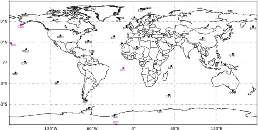
In this first TM5 CO inversion study, only surface observations from NOAA/ESRL GMD are assimilated in the 4D-VAR system. The NOAA surface network provides CO

ob-20

servations from a globally distributed network of stations (Novelli et al., 1998, 2003). A subset of 31 stations, mainly remote stations and stations at larger distances from continental source regions are used in the inversions. Stations close to source regions as well as other stations for which we expect large model errors due to the coarse model resolution are left out. The selected stations are shown in Fig. 1. The

observa-25

(12)

ACPD

11, 341–386, 2011

Title Page

Tables Figures

◭ ◮

Back Close

Full Screen / Esc

Discussion

P

a

per

|

Dis

cussion

P

a

per

|

Discussion

P

a

per

|

Discussio

n

P

a

per

|

error is set to 1.5 ppb. The model error in the vertical direction is based on the mod-eled CO mixing ratio gradient for the grid boxes adjacent to the one the station is in (Bergamaschi et al., 2005). For the horizontal model error, subgrid-scale variability of the emissions is accounted for as described in Bergamaschi et al. (2010). The model error is usually much larger than the measurement error for stations on the NH. Only

5

in remote areas in the SH, the measurement error is the dominant term in the obser-vational error. No correlations between the observations are set resulting in a diagonal observational error covariance matrixR.

2.5 Inversion specifics

In this study the simulations with TM5 are performed on a rather coarse 6◦×4◦

hori-10

zontal grid with 25 vertical layers. This means that after the application of emissions each time step, the CO mixing ratio is smeared out over the entire grid box. Hence, we do not expect the model to simulate all measured pollution events at non-background stations. To account for this and to prevent possible biases due to a few single outliers, the inversion is done in two cycles: After the first inversion we reject all data points

15

that are outside a 3σ error range of the model simulation (Bergamaschi et al., 2010). Then the second inversion cycle is performed. In the CH4 inversion of Bergamaschi

et al. (2010), typically 3% of the data were rejected, but the a posteriori emissions for both inversion cycles did not differ very much in general. However, in the current study, focusing on the shorter-lived CO, approximately 15–20% of the data from the first

inver-20

sion are rejected. Inferred continental emissions in the second cycle are within 15% of the emissions in the first cycle for most sources/regions and show a similar pattern of adjustments. However, biomass burning emissions for Africa and Asia may differ up to 30%. This is due to the low month to month correlation of biomass burning emissions and the sparsity of NOAA surface observations in these regions.

25

(13)

ACPD

11, 341–386, 2011

Title Page

Tables Figures

◭ ◮

Back Close

Full Screen / Esc

Discussion

P

a

per

|

Dis

cussion

P

a

per

|

Discussion

P

a

per

|

Discussio

n

P

a

per

|

inversion with more strict observational errors. This is illustrated by the behaviour of the cost function. The background part of the optimized cost function (first term in Eq. 2) amounts to 238 compared to 460 in the base inversion (presented in Sect. 3). The observational part of the cost function (second term in Eq. 2) amounts to 839 compared to 1139 in the base inversion, again due to the larger observational errors.

5

The years 2003 and 2004 are inverted separately because the inversions are computer-time demanding. The inversions use a one month spin up, in which the emissions are optimized already, but not analyzed, and 2 months spin down to supply enough observations to optimize the emissions in the last months of the year. Given a lifetime of about 2 months for CO, it has been investigated that to optimize emissions

10

in a certain monthm, it is su_fficient to use observations for monthsm,m+1 andm+2 (not shown). Observations at later times will not significantly influence the emissions in monthm, because the emission signal is sufficiently diluted and chemically removed by that time. It should be borne in mind, however, that emissions in monthm are still influenced by emission estimates in surrounding months (m−3,...,m+3) via the prior

15

temporal correlation length.

The length of the state vector is 189030, according to (15 months×3 source cate-gories+25 vertical layers of the initial concentration field)×(60×45 grid boxes)+

15 months×2 scaling factors. In contrast, the total number of observations is only about 1400 per year. By introducing a non-diagonal prior error covariance matrix, the

num-20

ber of “true” unknowns is greatly reduced to approximately 25 000, but the problem still remains underdetermined (data sparse and hence strongly dependent on a priori knowledge of the emissions). Nevertheless, a grid-scale inversion is performed here to reduce the risk of aggregation errors, which often occur in a big region approach (Meirink et al., 2008b; Stavrakou and M ¨uller, 2006) and to prepare for the future

inges-25

(14)

ACPD

11, 341–386, 2011

Title Page

Tables Figures

◭ ◮

Back Close

Full Screen / Esc

Discussion

P

a

per

|

Dis

cussion

P

a

per

|

Discussion

P

a

per

|

Discussio

n

P

a

per

|

3 Inversion results

3.1 Comparison of modeled and observed CO mixing ratios

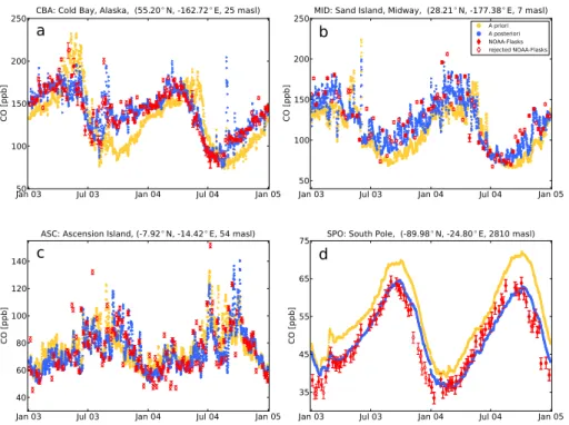
In this section we will discuss the capability of the current 4D-VAR system to adjust the state vector in such a way that background CO mixing ratios as well as observed large scale pollution events are adequately captured. Figure 2 shows the prior and

5

posterior simulation of CO mixing ratios and surface observations for a subset of four stations used in the inversion (purple squares in Fig. 1). All panels show that the model simulation with a priori settings (yellow) is capable to simulate the seasonal cycle and some pollution peaks even though the simulations are performed on a coarse 6◦×4◦ grid. However, differences with the observations (red) up to 50 ppb are observed. In

10

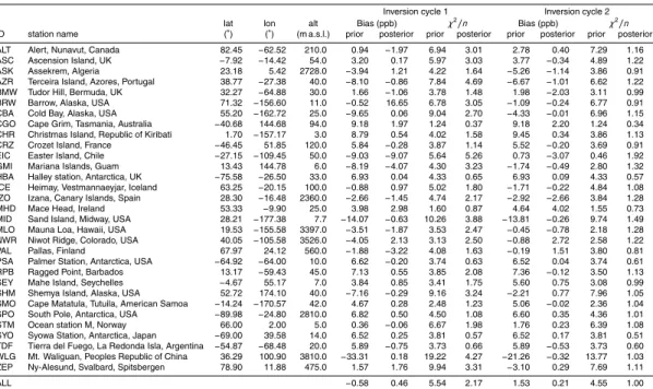
contrast, the posterior simulation (blue) fits the observations at all four stations rather well. This better fit is obviously caused by combined changes in the surface emissions and in the global source of CO from methane and NMVOCs. A quantitative analysis for all assimilated stations is shown in Table 1 for 2004. Here we present the bias per station for the prior and posterior simulation of the two inversion cycles. A value for

15

the goodness of fit parameterχ2/nis also given in this table. Aχ2/nvalue close to 1 indicates that the system is behaving well.

For station Cold Bay, Alaska (Fig. 2a), representing the high latitude NH, the prior simulation underestimates observed CO mixing ratios up to 50 ppb, in the period September 2003 to February 2004 and from September 2004 to January 2005. For

20

the year 2003, the inversion decreases biomass burning emissions from Russia in spring, but emissions are increased in summer. The posterior annual biomass burn-ing emission estimate for Russia in 2003 is 97±28 Tg CO (compared to the prior es-timate of 75±77 Tg CO), well within the range reported by Kasischke et al. (2005) (55–139 Tg CO yr−1). This shows that Russian fires account for 60% of the total CO

25

(15)

ACPD

11, 341–386, 2011

Title Page

Tables Figures

◭ ◮

Back Close

Full Screen / Esc

Discussion

P

a

per

|

Dis

cussion

P

a

per

|

Discussion

P

a

per

|

Discussio

n

P

a

per

|

36±9 Tg CO as posterior emission estimate. This increase in Alaskan and Canadian biomass burning emissions was also reported by Pfister et al. (2005) and Turquety et al. (2007), and in closer correspondence to 30 Tg CO as estimated in the recently released updated GFED (version 3.1, van der Werf et al., 2010). Pfister et al. (2005) inferred CO emissions using satellite observations and reported a posterior emission

5

estimate of 30±5 Tg CO. Turquety et al. (2007) constructed a daily biomass burning emission inventory taking into account the emissions from peat burning. They esti-mated a total of 30 Tg CO from June to August 2004 for North America. Outside the biomass burning season, the inversion attributes increased CO levels to enhanced an-thropogenic emissions in East Asia. From Table 1 it is observed that for station Cold

10

Bay the prior bias decreases from −9.7 ppb in the first inversion cycle to −4.3 ppb in the second inversion cycle due to rejection of observations that are not reproduced by the model. This rejection improves the a posterioriχ2/ndiagnostic for this station from 2.7 to 1.15. The posterior bias is reduced to nearly zero.

For station Sand Island, Midway (Fig. 2b), the prior simulation underestimates

obser-15

vations during the entire period. This was expected due to the use of the EDGARv3.2 inventory (compiled for the year 1995) for anthropogenic emissions for this region for the years 2003 and 2004. Rapid economic development, particularly in China and India over the last decade led to increased anthropogenic emissions. The posterior simulation shows that increased anthropogenic emissions over China and India (the

20

inversion roughly doubles Asian anthropogenic emissions, see Table 2) results in 15– 25 ppb higher CO mixing ratios on stations downwind of South East Asia. Individual observations due to pollution plumes that were not reproduced in the prior simulation are captured better by the model in the posterior simulation. This is due to the fact that the 4D-VAR system computes emission increments on the grid-scale of the underlying

25

(16)

ACPD

11, 341–386, 2011

Title Page

Tables Figures

◭ ◮

Back Close

Full Screen / Esc

Discussion

P

a

per

|

Dis

cussion

P

a

per

|

Discussion

P

a

per

|

Discussio

n

P

a

per

|

The tropics are represented here by station Ascension Island (Fig. 2c), and although the improvement from prior to posterior simulation is not clearly visible, Table 1 shows that the posterior bias is nearly zero, and theχ2/ndiagnostic is reduced from 3.03 to 1.22. For the remote SH, represented here by station South Pole (Fig. 2d), the prior simulation overestimates the observations by 5–10 ppb all year long. The inversion

5

attributes this to too high production of CO from NMVOCs since the station is far away from major sources, but neglecting the N-S gradient in tropospheric methane in the model, as discussed before, may also play a role. Again, the posterior bias is nearly zero in both inversion cycles and theχ2/ndiagnostic obtains a value of 1.01.

Table 1 shows that the inversion reduces prior biases for most of the stations and

10

that theχ2/ndiagnostic is decreased to approximately 1. However, for remote stations in the SH,χ2/nshows values far smaller than 1 indicating that the measurement error of 1.5 ppb might be too conservative or indicating the need to take correlations in the observation errors into account.

3.2 Posterior emission estimates

15

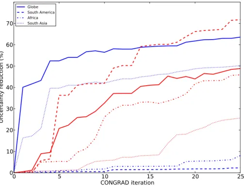
We present the posterior emission estimates and their uncertainties aggregated over continental scale regions as yearly totals, because the monthly emission estimates on grid-scale level are highly variable as a consequence of the loose prior error settings and the small amount of observations. Also, as shown by Meirink et al. (2008b), the posterior errors converge only rapidly for larger spatial and temporal scales (Fig. 3).

20

Table 2 and Fig. 3 (blue, solid line) show that on a global scale, a substantial un-certainty reduction of 60% for the anthropogenic emissions is achieved. Columns 2 and 3 of Table 2 show that in particular Asian anthropogenic emissions are well con-strained by the observations (258±150 Tg CO a priori compared to 497±82 Tg CO in 2003 and 526±75 Tg CO in 2004 a posteriori, see also Fig. 3, dotted blue line). In

con-25

(17)

ACPD

11, 341–386, 2011

Title Page

Tables Figures

◭ ◮

Back Close

Full Screen / Esc

Discussion

P

a

per

|

Dis

cussion

P

a

per

|

Discussion

P

a

per

|

Discussio

n

P

a

per

|

error reduction in those regions is largest for the dominant biomass burning source term.

For biomass burning emissions, uncertainty reduction is achieved in South America (e.g., 98±105 Tg CO a priori compared to 136±39 Tg CO a posteriori in 2004, Fig. 3 red dashed line), Asia (e.g., 114±81 Tg CO a priori compared to 158±38 Tg CO in 2003

5

(not shown)) and North America (23±19 Tg CO a priori and 47±10 Tg CO a posteriori in 2004 only). Large changes in biomass burning emissions from 2003 to 2004 are ob-served for South America and Africa. For South America (with posterior emissions of 75±37 Tg CO in 2003 and 136±39 Tg CO in 2004) this increment was partly present in the GFED2 prior. Higher emissions in 2004 were also confirmed by observations from

10

the Scanning Imaging Absorption Spectrometer for Atmospheric Cartography (SCIA-MACHY) (Gloudemans et al., 2009) showing the large inter annual variability in South American biomass burning emissions. In contrast, the posterior biomass burning emis-sion estimates for Africa in 2003 and 2004 seem to compensate for the di_fference in NMVOC-CO. This is confirmed by the relatively small error reduction and by the study

15

of Chevallier et al. (2009), who optimized African emissions using MOPITT observa-tions for 2000 to 2006 and did not show large inter annual variability from 2003 to 2004. Table 2 (columns 6 and 7) shows that natural emissions are hardly constrained by the data.

Finally, the uncertainty of the global scaling parameters for the production of CO from

20

methane and NMVOC oxidation is only slightly reduced from the prior to the posterior estimate. This indicates that the current observational dataset does not constrain these parameters substantially. However, the value of the scaling factor for the NMVOC-CO (NMVOC-CO from NMVOCs) source is adjusted significantly from a prior global total of 812±40 Tg CO to a posterior global total of 574±38 Tg CO in 2003 and 410±36 Tg CO

25

(18)

ACPD

11, 341–386, 2011

Title Page

Tables Figures

◭ ◮

Back Close

Full Screen / Esc

Discussion

P

a

per

|

Dis

cussion

P

a

per

|

Discussion

P

a

per

|

Discussio

n

P

a

per

|

global parameter have a strong influence on the solution of the inversion. Sensitivity studies with respect to these error settings have been performed as discussed in more detail in Sect. 5.

3.3 Validation with independent NOAA aircraft observations and MOPITT total

columns

5

We validate our inferred emissions with independent (that is, non-assimilated) aircraft observations from the NOAA aircraft program for 2004. The comparison with aircraft data provides a valuable test for the vertical transport in the model. The NOAA pro-files are taken mainly over North America. Figure 4 shows monthly mean deviations (model-observations) for the prior and posterior simulation for aircraft samples with

10

altitudes above 2000 m, thus representing the free troposphere. The prior simulation underestimates the observations throughout the year (except for May and June) proba-bly due to too low anthropogenic emissions in East Asia. The significant overestimation of the prior simulation in May and June is attributed to a too large a priori source of CO from NMVOCs. The posterior simulation matches the observations much better, since

15

the inversion increased Asian anthropogenic emissions and reduced the NMVOC-CO source (Table 2), in particular in May and June (not shown). The uncertainty, given here as a 1σ deviation from the mean, is not reduced significantly from prior to pos-terior simulation because these observations are not assimilated. Overall, the mean monthly difference is reduced by 50–90% except for April when deviations were small

20

anyway. The annual mean and standard deviation of the residuals is −6.4±23 ppb a priori and−0.5±22 ppb a posteriori, showing that the inversion is capable to improve the comparison with independent observations in the free troposphere.

We further validate our posterior emissions with CO total column retrievals from MO-PITT V4 (level 3, gridded daily profiles, Deeter et al., 2003, 2007, 2010). The MOMO-PITT

25

(19)

ACPD

11, 341–386, 2011

Title Page

Tables Figures

◭ ◮

Back Close

Full Screen / Esc

Discussion

P

a

per

|

Dis

cussion

P

a

per

|

Discussion

P

a

per

|

Discussio

n

P

a

per

|

the MOPITT averaging kernels are used to compare properly. Surprisingly, the overall agreement with MOPITT seems to deteriorate from the prior to the posterior simulation. However, over the well-constrained NH, the agreement improves slightly for 2004 from a prior underestimate of 12% to a posterior overestimate of 6%. Over the continents, the agreement improves even more. For 2003, the prior simulation underestimates

5

MOPITT by 8% but the posterior simulation overestimates MOPITT by 13%. In the re-mote SH (30◦to 62◦S), the comparison with MOPITT deteriorates from a slight model underestimate of 6% a priori to an underestimate of 40% a posteriori in both years. The prior simulation overestimates surface observations of CO at the remote SH stations (see Fig. 2d). These SH surface observations thus cause a decrease in CO sources

10

(mainly NMVOC-CO) which results in even less CO compared to MOPITT. The un-derestimation of the model may have to do with the vertical transport in the model. For instance, if vertical transport in the model is too slow, CO emissions will remain at low altitudes where the MOPITT instrument is not very sensitive. The comparison with NOAA aircraft profiles showed however that the vertical transport in TM5 is

rea-15

sonable. Hence, a possible bias in the MOPITT V4 product as was the case for the previous product MOPITT V3 (Emmons et al., 2009; de Laat et al., 2010) may also play a role. The suspect land-sea differences in Fig. 5, especially in the vicinity of desert regions indeed indicate that not all retrieval issues may have yet been resolved.

In conclusion, validating our inversion results with independent aircraft data shows an

20

improved agreement with respect to the prior simulation in the free troposphere even though only surface observations are assimilated. For satellite data, the agreement with MOPITT total column CO shows a slight improvement over the well-constrained NH, but deteriorates in the SH below 30◦S.

3.4 Comparison with recent inverse modeling results

25

(20)

ACPD

11, 341–386, 2011

Title Page

Tables Figures

◭ ◮

Back Close

Full Screen / Esc

Discussion

P

a

per

|

Dis

cussion

P

a

per

|

Discussion

P

a

per

|

Discussio

n

P

a

per

|

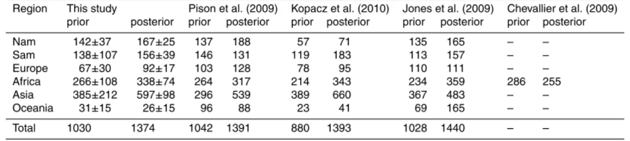
optimization by assimilating methyl chloroform observations. Results are comparable to our results, but slightly higher for Europe and lower for South America. However, the Australian source of Pison et al. (2009) included CO emissions from Indonesia and is thus significantly higher than the current study. Kopacz et al. (2010) used satellite data (from MOPITT, the Atmospheric Infrared Sounder (AIRS) instrument and

SCIA-5

MACHY) to optimize CO emissions for the period May 2004 to April 2005 and their results showed slightly higher emissions over South America and Asia, but significantly lower emissions over North America. This might be due to their very low prior value for anthropogenic emissions over the United States (35 Tg CO) based on the US Envi-ronmental Protection Agency National Emission Inventory for 1999 (EPA NEI99). This

10

value was decreased by 60% following Hudman et al. (2008). In this study we use 105 Tg CO as prior anthropogenic emission over North America. Jones et al. (2009) optimized emissions for November 2004 only using observations from the MOPITT and TES instruments, but they presented their results as yearly totals. These results are also comparable to the current study except for the Australian source. This is explained

15

by their inclusion of Indonesia into this region. Chevallier et al. (2009) have performed a detailed analysis of African CO emissions for the period 2000–2006. The total emis-sions are 25% lower than in this study but stay well within the error bounds. The dif-ference with our results is probably explained by the lack of surface data in the tropics. Chevallier et al. (2009) used MOPITT data to constrain the CO emissions and

anthro-20

pogenic emissions in particular were more constrained than in the current study. Fi-nally, the large increment in Asian anthropogenic emissions shown in Table 2 also con-firms the previous findings of e.g., Kasibhatla et al. (2002) and Arellano et al. (2004) that anthropogenic emissions over Asia are too low in EDGARv3.2. All inversions roughly doubled the Asian emission estimate.

(21)

ACPD

11, 341–386, 2011

Title Page

Tables Figures

◭ ◮

Back Close

Full Screen / Esc

Discussion

P

a

per

|

Dis

cussion

P

a

per

|

Discussion

P

a

per

|

Discussio

n

P

a

per

|

4 Discussion

In our inversions we have used a limited amount of observations from the NOAA sur-face network. A consequence of solving a data sparse system is a large solution space, because not all degrees of freedom (≈25 000) are constrained by the observa-tions (≈1400 per year). Thus, the obtained solution will depend on the prior emissions

5

and their error settings. Another consequence might be that model errors are compen-sated for by emission increments. To investigate these issues, a series of sensitivity studies is presented in Sect. 5.

The 4D-VAR system is in general not capable to distinguish between the an-thropogenic, biomass burning and the NMVOC-CO sources. Although globally the

10

posterior source estimate for these three sources is 1744±76 Tg CO in 2003 and 1690±75 Tg CO in 2004 and the difference is well within the error bounds, in partic-ular anthropogenic emissions and the NMVOC-CO source show large shifts from 2003 to 2004. Some of these shifts seem not driven by observations, but rather a compen-sation for a change in another source. For example, the derived NMVOC-CO source

15

shows a large drop from 2003 to 2004 (574 Tg CO in 2003 to 410 Tg CO in 2004), which seems to be an artefact of the system rather than a real signal of reduced NMVOC-CO, caused by the design of the system. Since the global NMVOC-CO source is scaled by a monthly varying parameter, the large changes in these parameters have only little ef-fect on the background part of the cost function (Eq. 2 left-hand term), but a huge effect

20

on the observational part of the cost function (Eq. 2 right-hand term) in particular in the SH. This drop is compensated (within the error bounds) by increased anthropogenic emissions (770 Tg CO in 2003 to 871 Tg CO in 2004). We calculated the posterior cor-relation (from the posterior covariance matrix A, Eq. 2) between the two sources to be negative (−0.29 in 2003 and −0.23 in 2004), further indicating this compensation

25

(22)

ACPD

11, 341–386, 2011

Title Page

Tables Figures

◭ ◮

Back Close

Full Screen / Esc

Discussion

P

a

per

|

Dis

cussion

P

a

per

|

Discussion

P

a

per

|

Discussio

n

P

a

per

|

burning emissions in 2003 increase without a reduction in the error from 32±32 Tg CO to 61±30 Tg CO (Table 2). Hence, the increase seems a further compensation for the reduction in the NMVOC-CO source.

For specific regions where biomass burning emissions are the dominant source (e.g., South America), the 4D-VAR system appears to be capable to distinguish biomass

5

burning emissions from the anthropogenic source. This is probably caused by the timing of these emissions as proposed by the prior inventory and the low month to month temporal correlation used. An example of this differentiation between anthro-pogenic and biomass burning sources is observed for North America and South Amer-ica in 2004. Although anthropogenic source estimates show no uncertainty reduction

10

and are equal or slightly smaller than the prior estimate, biomass burning emissions increase from the prior emission estimate and the posterior emission uncertainty is reduced significantly. In 2003 this is also observed in South America, where anthro-pogenic emissions are even reduced to non-significant negative values (Table 2), while biomass burning emissions increase from 60±48 to 75±37 Tg CO yr−1.

15

5 Sensitivity analysis

In this section we discuss 7 sensitivity studies with respect to prior settings and model errors. Sensitivity studies S1–S4 focus on the effect of the prior grid-scale error for the surface emissions and the prior NMVOC-CO error on the derived posterior emissions. Study GFED3.1 uses the new version of the GFED product (GFEDv3.1, van der Werf

20

et al., 2010). For the year 2004, this biomass burning inventory prescribes lower emis-sions by a factor 2 to 3 from January to March compared to GFED2. Peak emisemis-sions in September in GFED2 of 69 Tg CO/month globally are reduced to 55 Tg CO/month in GFED3.1.

Since the distribution of OH and its north-south gradient remains uncertain, we also

25

(23)

ACPD

11, 341–386, 2011

Title Page

Tables Figures

◭ ◮

Back Close

Full Screen / Esc

Discussion

P

a

per

|

Dis

cussion

P

a

per

|

Discussion

P

a

per

|

Discussio

n

P

a

per

|

2010) and scaled by a factor 1.02 to obtain comparable CO and methyl chloroform lifetimes as for the OH field used in the base inversion. Compared to the OH field of the base inversion, the north-south gradient (computed as an airmass-weighted average (Lawrence et al., 2001)) in the TM5-OH field is more pronounced (NH/SH ratio of 1.15) compared to the OH field used in the base inversion (NH/SH ratio of 1.0).

5

Study FVERT focusses on model uncertainty in the vertical distribution of biomass burning emissions. The base inversion uses an injection height for biomass burning emissions up to 2000 m (distributed as 20% in layers 0–100 m, 100–500 m and 500– 1000 m and 40% in 1000–2000 m layer). However, some recent studies (Gonzi and Palmer, 2010; Val Martin et al., 2009) found evidence that biomass burning emissions

10

are partly injected higher up in the atmosphere. In study FVERT we apply a vertical distribution of biomass burning emissions following the results of Gonzi and Palmer (2010). The vertical biomass burning emission distribution is defined as

– Boreal region (>30◦N): 82% below 2 km, 10% in 2–5 km, 2.5% in each of the layers 5–8 km and 8–11 km. The remaining 3% is injected above 11 km.

15

– Tropical region: 85% below 2 km, 10% in 2–5 km, 2.5% in both layers 5–8 km and 8–11 km.

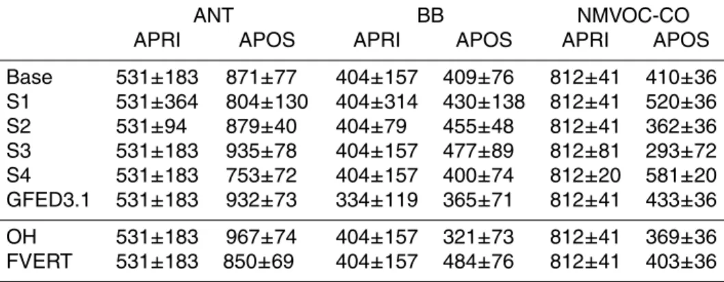
A summary of the sensitivity studies is provided in Table 4. The inversion results for these sensitivity tests are averaged globally for 2004 and are summarized in Table 5, where we omit the natural emissions and CH4-CO since these sources do not change

20

significantly from the prior to the posterior emission estimates in the base inversion.

5.1 Sensitivity studies S1–S4

Overall, the inferred anthropogenic and biomass burning emissions for studies S1 to S4 (Table 5) are quite robust as nearly all posterior emission estimates are within the error bounds of each other. The differences in emission estimates for S1 to S4 are likely

25

(24)

ACPD

11, 341–386, 2011

Title Page

Tables Figures

◭ ◮

Back Close

Full Screen / Esc

Discussion

P

a

per

|

Dis

cussion

P

a

per

|

Discussion

P

a

per

|

Discussio

n

P

a

per

|

before. This compensation mechanism depends on the combination of the prior er-rors in the anthropogenic and NMVOC-CO emissions. For example, in sensitivity study S1, the NMVOC-CO prior error dominates, resulting in less reduction in this source compared to the base inversion. The anthropogenic source compensates for this by reducing the emission estimate with 67 Tg CO yr−1compared to the base inversion. In

5

contrast, for sensitivity study S3, the anthropogenic emission prior error dominates, resulting in higher anthropogenic emissions and a more pronounced reduction in the NMVOC-CO source compared to the base inversion. Biomass burning emission es-timates are only slightly sensitive to the prior error settings, as all sensitivity studies estimate posterior biomass burning emissions in the range 400–477 Tg CO yr−1.

10

We conclude that anthropogenic emissions and the NMVOC-CO source can not be properly separated by assimilation of a limited number of observations. The situation will likely improve when we start the assimilation of large amounts of satellite data in our system. However, a separation between di_fferent source categories will remain extremely challenging and might require additional information from other sources. For

15

example, satellite observations of formaldehyde and glyoxal may further constrain the distribution of NMVOCs (Stavrakou et al., 2009).

5.2 Sensitivity study GFED3.1

The results for sensitivity study GFED3.1 (Table 5) show an increase in biomass burning of 30 Tg CO yr−1 with respect to the prior estimate of 334 Tg CO yr−1.

20

Biomass burning emissions mainly increase in South America (₊45 Tg CO yr−1) and Africa (+9 Tg CO yr−1). However, Asian biomass burning emissions decrease by 32 Tg CO yr−1. This behavior was also observed for the base inversion. For exam-ple, for the base inversion the increase in South America was 38 Tg CO, whereas for Africa there was no significant increase. Asian biomass burning emissions decreased

25

(25)

ACPD

11, 341–386, 2011

Title Page

Tables Figures

◭ ◮

Back Close

Full Screen / Esc

Discussion

P

a

per

|

Dis

cussion

P

a

per

|

Discussion

P

a

per

|

Discussio

n

P

a

per

|

waste burning and deforestation fires (van der Werf et al., 2010). To compensate for the lower biomass burning emissions, anthropogenic emissions (932±73 Tg CO) and the NMVOC-CO source (433 Tg CO) are increased with respect to the base inversion.

5.3 Sensitivity study OH

The OH field from the TM5 full-chemistry simulation shows lower OH over tropical land

5

masses compared to the OH field from Spivakovsky et al. (2000) (Fig. 6, top), in par-ticular over South America. This OH gap is present since large amounts of emitted isoprene are oxidized by OH and hence reduce OH concentrations in the model. How-ever, as shown by Lelieveld et al. (2008), this OH gap is not confirmed by field cam-paigns that show high OH over the tropical forests. An OH recycling mechanism was

10

proposed by Lelieveld et al. (2008), but was not yet incorporated in the TM5 simula-tion (Huijnen et al., 2010). Lower OH concentrasimula-tions over tropical land masses (Fig. 6, top) result in a reduction of biomass burning emissions of 88 Tg CO yr−1 globally in 2004 compared to the base inversion (Table 5, Fig. 6 bottom). Africa (−51 Tg CO yr−1) and South America (−30 Tg CO yr−1) contribute substantially to this decrease. The

15

NMVOC-CO source is reduced to 369 Tg CO yr−1, which is 41 Tg CO yr−1lower than in the base inversion. This reduction is also attributed to the lower OH concentrations in the SH. In contrast, the NH OH concentration is higher compared to the OH field from Spivakovsky et al. (2000). Therefore, higher global anthropogenic emissions are ob-served for this study (967 Tg CO yr−1) compared to the base inversion (871 Tg CO yr−1).

20

This di_fference is clearly observed over India in Fig. 6. The comparison with MOPITT is not improved with respect to the base inversion (not shown): The remote SH still shows an underestimate of MOPITT total columns.

5.4 Sensitivity study FVERT

When biomass burning CO emissions are released higher up in the atmosphere, one

25

(26)

concen-ACPD

11, 341–386, 2011

Title Page

Tables Figures

◭ ◮

Back Close

Full Screen / Esc

Discussion

P

a

per

|

Dis

cussion

P

a

per

|

Discussion

P

a

per

|

Discussio

n

P

a

per

|

trations of biomass burning CO decrease and thus, higher CO surface emissions are required to match the observations. Indeed, it is observed that the global biomass burning emissions increase with 75 Tg CO yr−1 with respect to the base inversion (Ta-ble 5). Moreover, this increase is only partly compensated for by decreased an-thropogenic emissions (−21 Tg CO yr−1) and a decrease in the NMVOC-CO source

5

(−7 Tg CO yr−1), indicating that a part of the biomass burning CO emissions is not de-tected by the surface network. Higher biomass burning CO emissions with respect to the base inversion cause the comparison with MOPITT CO total columns to change: Over the main biomass burning regions in Africa, South America and South East Asia, the comparison deteriorates, because the base inversion already overestimates

MO-10

PITT CO total columns over these regions (Fig. 5d). On the remote SH, the comparison does not change significantly since the NMVOC-CO source shows only minor changes with respect to the base inversion. We conclude that the biomass burning injection height is a potentially important parameter to take into account in inversions. However, the agreement with MOPITT CO on the SH total columns does not improve, mainly

15

because it seems that the surface observations and MOPITT CO total columns are not consistent in the model. This was also observed by Kopacz et al. (2010). They inverted CO emissions using satellite data only and SH stations used as validation showed a poorer agreement in the posterior simulation compared to the prior.

The planned assimilation of MOPITT CO total columns may result in a less

pro-20

nounced reduction in the NMVOC-CO in order to fit the satellite data. In turn, more NMVOC-CO may result in lower biomass burning emissions and hence, an improved agreement over the main biomass burning regions in the SH. Moreover, biomass burn-ing emissions might become more comparable with the new GFED3.1 (van der Werf et al., 2010) product. However, when assimilating both MOPITT CO total column data

25

(27)

ACPD

11, 341–386, 2011

Title Page

Tables Figures

◭ ◮

Back Close

Full Screen / Esc

Discussion

P

a

per

|

Dis

cussion

P

a

per

|

Discussion

P

a

per

|

Discussio

n

P

a

per

|

6 Conclusions

We have presented a 4D-VAR data assimilation system for CO using simplified chem-istry and a fixed OH field, meant to assimilate large satellite datasets, but tested here using surface network observations from NOAA only. The proper functioning of the system is shown by the fact that the posterior simulation reproduces background CO

5

mixing ratios including events with enhanced CO mixing ratios. The mean bias between modeled CO mixing ratios and observations from the NOAA surface network reduces for nearly all stations and theχ2/ncharacteristic is reduced to values around 1, indicat-ing that the chosen prior errors result in a well-balanced system. As expected, regions that are well constrained by the observational data show large uncertainty reductions,

10

whereas non-constrained regions show only minor error reductions.

Our annual continental emissions compare well with recent inverse modeling studies, indicating that the global budget of CO is well constrained in our inversion. The poste-rior emissions have been validated using non-assimilated aircraft data from NOAA and vertical column data from MOPITT V4. The forward simulation with the inferred

emis-15

sions showed much more resemblance with NOAA aircraft observations in the free troposphere compared to the prior simulation, showing that the inversion is capable to improve the free tropospheric CO distribution even though only surface observations are assimilated. The comparison with MOPITT total column CO improves slightly over the well-constrained NH from the prior to the posterior simulation. However, in the

20

SH, the comparison with MOPITT deteriorates from approximately a 6% low a priori to a 40% low a posteriori, due to an emission decrease forced by SH surface observa-tions.

With the limited amount of assimilated data and the low spatiotemporal resolution of surface network observations, it is difficult to distinguish between anthropogenic

25

(28)

ACPD

11, 341–386, 2011

Title Page

Tables Figures

◭ ◮

Back Close

Full Screen / Esc

Discussion

P

a

per

|

Dis

cussion

P

a

per

|

Discussion

P

a

per

|

Discussio

n

P

a

per

|

was confirmed by sensitivity studies. However, regions where the timing of the biomass burning emissions is very important (e.g., South America) show that it is possible to distinguish between anthropogenic and biomass burning emissions.

The impact of model errors on the inversion results was investigated by employing a di_fferent OH field and a di_fferent biomass burning emission height. An OH

distri-5

bution from a full-chemistry simulation with TM5 with a more pronounced N-S ratio in OH largely influenced the inversion results: Biomass burning emissions and NMVOC-CO reduced whereas the anthropogenic emissions increased compared to the base inversion. This shows that the OH distribution over the NH and SH is critical for CO inversions. For this OH field the comparison with MOPITT total column CO in the SH

10

did not improve and even less CO emissions were inferred on the SH. The sensitivity study with a different biomass burning injection height showed that the vertical distribu-tion of biomass burning also largely influences the inversion results. Biomass burning emissions increased by 75 Tg CO yr−1 with respect to the base inversion. Again, the comparison with MOPITT total columns did not improve. Increased biomass burning

15

emissions over emission hotspots in South America, Central Africa and Indonesia re-sult in an even larger discrepancy with MOPITT total columns. On the remote SH the comparison with MOPITT was similarly poor as in the base inversion.

The use of satellite data in combination with the network of surface observations is an obvious next step. Assimilation of MOPITT total column CO is expected to lead to more

20

NMVOC-CO on the remote SH, which in turn might reduce biomass burning emissions over the fire hotspots in the SH. Lower biomass burning emissions will be more in line with the new GFED3.1 product. However, surface and satellite observations over the remote SH may bring conflicting information. Therefore, like in the assimilation of SCIAMACHY methane observations (Bergamaschi et al., 2009) a bias correction

25

scheme for satellite data seems necessary.