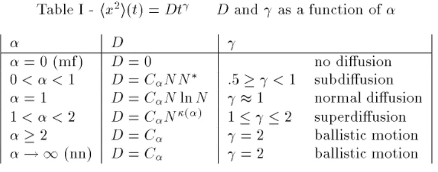
Nonextensive Eects in Tight-Binding Systems
with Long-Range Hopping
Lisa Borland 1
and J.G. Menchero 2 1
CentroBrasileirodePesquisasFisicas(CBPF), RuaDr. XavierSigaud150,22290-180RiodeJaneiro,Brazil.
2
InstitutodeFisica,UniversidadeFederaldo RiodeJaneiro, Cx. P.68.528,21945-970RiodeJaneiro,Brazil
Received 07 December, 1998
Consequences of long-range hopping in one-dimensional tight-binding models are studied. A hop-ping term proportional to 1=r
ij is used, where r
ij denotes the distance between atoms
i and j
anddetermines the range of the interactions within the system. Calculations of the diusion of
an electron along the lattice yield interesting eects of nonextensivity. In particular, we nd that the mean square displacement scales anomalously as D t
in the following way: For 0
< <1,
we ndD/NN
, where
N is the number of atoms on the lattice andN = N
1, ,1
1, is related
to the number of elements interacting at a given . In this regime the behaviour is subdiusive
(:5 <1) but approaches normal diusion ( = 1) for= 1. There exists a transition region
between 1<<2, where the diusion coecient loses its system size dependency and becomes
size independent for all 2. In addition, we nd 1<2 (superdiusion) for>1. Ballistic
motion ( = 2) is recovered for all1:5 and is maintained in the nearest neighbour limit.
Spe-cic heat and internal energy as a function of temperature and system size are also analyzed. They appear extensive on the macroscopic level for all values of.
I Introduction
There is a current interest in studying systems with long-range microscopic interactions. Indeed, they have been found to exhibit a variety of interesting properties, ranging from nonextensive thermodynamic behaviour to anomalous diusion and anomalous Lyapunov expo-nents ([1, 2, 3] and references therein). These results all imply that it may be neccessary to rethink the standard formulation of thermodynamics, which seems to break down when it comes to the description of this vast class of physical systems.
The generalized nonextensive thermostatistics re-cently proposed by Tsallis [4] has proven to be a suc-cessful candidate for treating a growing body of sys-tems for which the standard thermodynamic formal-ism fails, and it appears to be that this is the frame-work neccessary to treat systems with long-range forces as well. Examples of situations where the generalized thermostatistics has been successfully applied { both theoretically and experimentally { are given by self-gravitating systems [5], two-dimensional turbulence in pure-electron plasma [6], the solar neutrino problem [7],
nonlinear maps [8], anomalous diusion of Levy type [9] and correlated type [10] to name just a few.
In this paper we wish to study the eects of long-range hopping in a simple one-dimensional quantum mechanical tight-binding model of electrons on a lat-tice of atoms (see also [11]). This should be interest-ing since it is a quantum mechanical system and, al-though some studies for tight-binding electron models with long-range hopping do exist [12, 13], most of the systems studied with long-range interactions which we are aware of have been classical. Furthermore, models with long-range interactions have a close resemblence to other interesting physical problems as diverse as the Kondo eect [14] and neural systems modeling [15].
First, we shall give a brief background concerning certain scaling laws which have recently been proposed by Tsallis [16] for nonextensive systems. It is suggested that the integral
N =
d Z
N 1=d 1
dr r d,1
r
,=
N 1,=d
,1 1,=d
(1) governs the thermodynamic scalings of systems with power-law decaying interactions of type 1=r
is the system size, d the dimension of the problem, r a distance, and a real number which determines the range of the interactions. In the limit N ! 1, N
behaves as
1
=d,1 ; =d > 1 ;
(2)
lnN ; =d = 1 ; (3)
N1,=d
1,=d ; 0
=d < 1: (4)
It has been shown [16] that these conditions imply that the classical system is thermodynamically exten-sive for =d > 1, wheras it becomes nonextensive for 0 =d 1, and special scalings become necessary in order to have a mathematically and physically well-posed problem. For one-dimensional classical systems (d = 1), we expect the crossover from the extensive to the nonextensive regime to occur at the critical value = 1. Forquantumsystems, it is as yet not quite clear where this crossover will occur. In addition, we point out that N is essentially proportional to the number of elements interacting within the system at a partic-ular range of the interactions, that is, at a particpartic-ular value of . This can be seen most simply for d = 1, as N =
RN 1 drr
, becomes just the integral of the probability r, of a particle interacting with another at distance r.
II The Model
The system under study is a one-dimensional tight-binding model of electrons on a lattice with N atomic sites, with a basis set of one s orbital per site. The tight-binding assumption implies that the electrons are localized on the lattice sites i, and the corresponding Hamiltonian has the form
H =XN
i ic
+
i ci+ N
X
i;j6=i V rijc+
i cj+ cc:: (5)
Here, the c+
i and ci are creation and anhilation
oper-ators for electrons on site i and the i are the on-site
energies, which are all set to zero. The power-law term V=rij describes the hopping of an electron from site i to site j. With a lattice spacing equal to unity, the dis-tance rijwill be measured in integer units. The
param-eter dparam-etermines the range of the interaction between dierent sites. It is clear that for !1we retrieve the conventional nearest neighbour (nn) model, whereas for = 0 we obtain the mean-eld limit where the electron can hop with equal probability to all sites.
III Static and Thermodynamic
Properties
I I I.1 EnergyEigenvalues
If we impose periodic boundary conditions then we obtain the following analytic expression for the energy eigenvalues:
Ek= 2V X
n=1
cos(kn)
n ; (6)
with k = ,2(m,1)=N and m = 1;;N. Here, n corresponds to the integer distance between two sites i and j. We assume that N is an even number, and if we only consider the shortest distance between sites then the summation goes to N=2 and one must subtract o half of the last term to avoid double counting.
We would like to point out that even though the re-sults we obtain are almost exactly the same regardless of whether we use periodic boundary conditions or not, we choose to not use periodic boundary conditions in this paper. This is mainly because there may be some mathematical artifacts introduced when periodicity is imposed on systems with long-range interactions, which we wish to avoid. We will use Eq (6) only to illuminate some of our discussion later on. So instead of calculat-ing the energy spectrum accordcalculat-ing to Eq (6), we nd the energies by numerically diagonalizing the hopping matrix occurring in the Hamiltonian Eq (5).
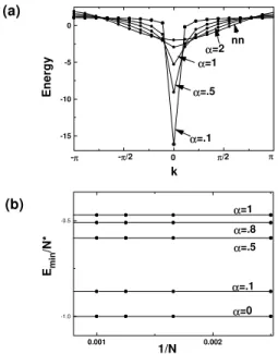
The results are shown in Fig. 1a, where we see the energy eigenvalues for a few dierent values of the pa-rameter , using a xed number of atoms. The results obtained by the analytic formula in Eq (6) are very similar. Notice that for 1, the lowest energy value Eminin the spectrum diverges, while all the others stay
nite. We found that as the system size N increases, the rate of this divergence scales exactly with the vari-able N of Eq(1) leaving E
min=N constant for each value of 1. This result is shown in Fig. 1b, and can be more easily understood with the aid of Eq (6). There we see that Emin is obtained for k = 0, when
all atoms are interacting constructively with all other atoms. This results in the energy term equal to
Ek= 2V X
n=1 1
n; (7)
the other eigenvalues, there are both constructive and destructive contributions to the total energy due to the dierent phase factors. Therefore, these do not diverge with increasing N but stay nite even for1. It is worth remarking that this behaviour is very dierent from what would have been expected in most classical cases, where we would have expected a situation where allthe energies diverge, and not just one.
π/2 -π/2 0 π -π
-15 -10 -5 0
0.001 0.002
-1.0 -0.5
(b) (a)
Energy Spectrum and Size Dependence
α=1
α=.5
α=.8
α=.1
α=0
Emin
/N*
1/N
Energy
k
α=.1
α=.5
α=1
α=2 nn
Figure 1. a) Energy levels for a system with 20 atoms (in units of 2V), calculated numerically without periodic boundary conditions, but plotted as a function of k =
(1,2(m,1)=N); m = 120. Here and in all
Fig-ures, nn denotes the nearest neighbour limit of ! 1.
Note that the lowest energy level Emindiverges for1,
while all other energies remain nite. b) We found that the lowest energy levelEmindiverges with system size such that Emin=Nis constant for each given value of
1. I I I.2 Sp ecicHeat andInternalEnergy
Now we shall calculate some thermodynamic quan-tities such as the specic heat and internal energy. Let us assume that the system consists of a lattice of size N atoms andN =2 electrons, neglecting spin. At tem-perature = 0 the internal energy is given by
U(0) =
N=2 X
i=1
Ei; (8)
where the N =2 electrons occupy all states up to the Fermi levelEF. At a given temperature the internal energy becomes
U() =
N
X
i=1
Eif(Ei) (9) which is simply the sum of energies of each state weighted by the probabilityf(Ei) of that state being occupied. Here,f(Ei) is given by the Fermi-Dirac dis-tribution (with the Boltzmann constantkB set to 1)
f(Ei) =
1
exp[(Ei,())=] + 1
; (10)
whereis the temperature dependent chemical poten-tial which can be determined implicitly by
N =2 =
N
X
i=1
f(Ei) =
N
X
i=1
1
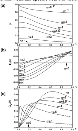
exp[(Ei,())=] + 1 : (11) We have plotted() in Fig. 2a, and in Fig. 2b we show U()=N for dierent N. First of all, note that the in-ternal energy U is an extensive variable for all values ofat all temperatures, resulting in data collapse for all values of N. There is no dependence on N
, even though we saw that the lowest energy Emin scales as N
with system size. This behaviour can be understood by rewriting the expression for the internal energy as U() =
PN
i=1
Eif(Ei) =E, PN
i=1
Ei(1,f(Ei)), where Eis the sum over all energy levels
PN
i=1
Eiand is equal to a nite constant which we have chosen to be 0. Now, Emin is so low that it is always occupied with proba-bilityf(Emin) = 1. However, in the second expression this implies thatEmin does not contribute to the sum at all. The internal energy is therefore determined only by the behaviour of all other energy levels, which re-main nite and well behaved. As was seen in the en-ergy spectrum (compare Fig. 1), those levels exhibit no noticeable change as we go from>1 to1, so it is not surprising that the same holds true for the internal energy. This result is very dierent from what we would have expected in the classical case, where it is predicted that the internal energy scales with the system size as U=(NN
0.0 0.2 0.4 0.6 0.8 1.0 -0.65 -0.60 -0.55 -0.50 -0.45 -0.40 nn
0.0 0.2 0.4 0.6 0.8 1.0 0.00 0.05 0.10 0.15 0.20 0.25 0.30 0.35 (c) (b) (a)
Chemical Potential, Specific Heat and Internal Energy
U/N τ NN α=2 α=1 α=.5 α=.2 α=.1 α=0 τ CV /N α=2 α=1.5 α=1 α=.5 α=.1 α=0 τ µ nn α=0 α=.1 α=.5 α=1 α=1.5 α=2 α=4
0.0 0.2 0.4 0.6 0.8 1.0 0.0 0.2 0.4 0.6 0.8 1.0
Figure 2: a) The chemical potentialis plotted as a function
of the temperature for dierent values of. The
temper-ature is expressed in fractions of the characteristic
inter-action energyV. b) The internal energyU=N is plotted as
a function of temperature for dierent values ofand N.
Again, all curves for dierent N coincide. c) The specic
heatC V
=Nas a function of temperature is shown for
dier-ent values ofand dierent values ofN. Note that there
is data-collapse for all N, implying that C
V is an
exten-sive variable. (The uctuations on the curves are numerical artifacts).
Next, we use the denitionCV =@(U()=@ in con-junction with Eq (9) to obtain the specic heat of the system. CV()=N is plotted in Fig. 2c for dierent values of. The curves for dierentN all coincide, im-plying thatCV() is an extensive variable scaling with N for all values of. The reason this is so despite the N
divergence of the lowest energy value is again be-causeEmin is always occupied, so that any changes in the internal energy due to temperature will only involve the well behaved nite energy levels. In any case, it is interesting to note the marked dierence in the temper-ature dependency of the specic heat for the dierent values of.
We calculated all of the above also using periodic boundary conditions, as well as varying the occupation level (i.e. number of electrons in the lattice). Neither
of these variations aected our results in any signicant way.
IV Dynamic Properties
IV.1 Disp ersionandDiusion
We now turn our attention from the static, thermo-dynamic properties to the thermo-dynamic, diusive properties of the system. In contrast to the extensive behaviour observed for the thermodynamic properties, the diu-sive properties show interesting nonextendiu-sive character-istics. There is a denite transition in behaviour as we go from the classically extensive (>1) to the classi-cally nonextensive (1) regime.
At timet= 0, a wavepacket may be expressed as
j (0)>=
N
X
i=1
aijfi>; (12) where theaiare the expansion coecients with respect to the localized basis set j fi >, which are essentially just the sites of the atoms. We choose to start out with localized on a single atom at siteN =2 in the middle of the lattice, so that only aN=
2
6
= 0 = 1. Alterna-tively, we can represent the wavepacket in terms of the energy eigenbasis which we nd numerically. Let us denote these eigenvectors byk,k= 1;N. Then we get
j (0)>=
N
X
k=1
bkjk> (13) with the expansion coecients bk =
PN
i=1
ai < k j fi>. The time evolution of this wavepacket is given by
j (t)>=
N
X
k=1
bk jk >eiE kt=
~
; (14)
which can be projected back onto the localized basis states to give the time-dependent amplitudesai(t) =<
(t)jfi>.
It is now straightforward to calculate the diusion, which we dene as the mean squared displacement of the position of the electron on the lattice. This is given by
<x 2
>(t) = X
i
x 2
i jai(t)j
2 (15)
wherejai(t)j
2gives the time-dependent probability of being on lattice site i, and xi is simply the positioni of the electron on the lattice, relative to the average position, i.e. xi=i,<i>with<i>=
P
IV.2 Diusion: Results andAnalysis
We expect the mean squared displacement of Eq (15) to follow the general diusion equation
<x 2
>(t) =D t
: (16)
Here, D is the diusion coecient and the temporal diusion exponent. If = 1 the diusion is said to be normal, if <1 the system is subdiusive and >1 means that the system is superdiusive. We shall now study the behaviour of both the diusion coecient D and the exponentfor dierent values ofand system size N.
Figure 3: The mean squared displacement <x 2
>(in units
of lattice spacings) is plotted as a function of time (tgiven
in units of~=V) for xed N = 800 and dierent . There
is a denite change in behaviour as crosses the critical
value of = 1. In the regime 01 the diusion goes
from subdiusive (<1) to normal ( = 1, i.e. increasing
linearly in time) yet with high-frequency oscillations. For
>1, the oscillations disappear but the diusion increases
parabolically in time ( > 1, superdiusion). A more
de-tailed analysis ofis presented in Figure 7.
First, we leave the system size N xed and calcu-late the diusion <x
2
>(t) according to Eq (15) for dierent values of. These results are shown in Fig. 3, for timescales short enough to exclude nite size eects which will be discussed in Fig. 4. In the mean-eld limit of = 0 the wavepacket remains primarily local-ized on the initial site, with small temporal oscillations
[13]. As a consequence the mean squared deviation <x
2
>(t) oscillates, but on the average the electron is trapped and does not diuse at all. For smallclose to 0 there is subdiusive behaviour ( <1), but as approaches 1 the diusion appears to increase more or less linearly with time, i.e. with 1. This corre-sponds to the case ofnormal diusion. However, as crosses the critical value of 1, the diusion is no longer linear in t. Instead it becomes parabolic, reaching a well-dened curve in the nearest-neighbour (nn) limit of!1. We shall consider the analysis of in more detail later on in Fig. 7. In addition, notice that all curves in the region1 exhibit high-frequency oscil-lating uctuations, whereas these disappear for>1. We conjecture that these oscillations are of a similar nature to those seen in the mean-eld limit.
It is clear from Fig. 3 that bothD and depend on, but let us now see how the diusion depends on N. To this end, we calculate the mean squared dis-placement<x
2
>(t) for dierent values ofand N, a representative subset of which is shown in Fig. 4. Log-log plots of<x
2
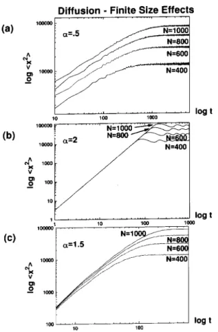
Figure 4: Log-log plots of the mean squared displacement (in units of lattice spacings) as a function of time (units of
~=V) are shown for dierent andN. The leveling o at
large times is a consequence of the nite-size boundary ef-fects. Our studies should therefore be done at intermediate times where these eects are negligible. a) Typical results for1. The curves are distinctly seperated for dierent N. b) Typical results for2. The diusion shows no size
dependency. c) There exists a transition region 1<<2
within which the curves lose their dependency on the system size N. Here at= 1:5 it is clear that the curves neither
coincide nor are quite distinctly seperated for dierentN. The question which we now pose is whether any scaling laws or data-collapse can be obtained for the N-dependent diusion curves. As shown in Fig. 5 this is achieved for all1 by plotting the quantity
<x 2
> NN
(17)
versus t for dierent values of N (here N between N = 200 and N = 1000). These results imply that the diusion coecient D scales as
D=C
NN
1; (18)
where C
denotes an
-dependent constant. To our knowledge, such a size-dependent scaling law is
re-ported for the rst time here and in [11]. In [13] a size-dependency for the diusion with= 1 was discussed where scaling of the form < x
2
> =N was suggested. For that particular value of this is a reasonable ap-proximation to our result Eq (18), which takes on the value <x
2
>=(NlnN) at = 1. But it is denitely less accurate, and not at all valid for any other values of.
Figure 5: The renormalized quantity < x 2
> =(NN ) is
plotted as a function of time (units of ~=V) for dierent
values of1 and N between 200 and 1000, resulting in
data-collapse for dierent N.
As was seen in Fig. 4b, there are no size-dependent eects in the region2. The diusion coecient can therefore be written as
D=C
2: (19)
However, as we cross over the critical value of = 1 into the regime 1 < < 2, neither the scaling laws of Eq (18) or Eq (19) are valid. Instead it seems as though there is a continuous transition in this regime, where the curves for dierent values ofNbecome closer and closer together until they collapse onto one at the value= 2. Data collapse was obtained empirically in this region, by renormalizing the diusion curves by the functionN
(), which is shown in Fig. 6. The function () was determined numerically from the data and is plotted in Fig. 6a. For = 1, N
() = N
1:16 which, for the sizes N analysed (up to 1000), is close to the result NN
=
observed for2. For largeN !1the scaling rep-resented by the function() will probably be an over-estimation of the true size dependence. This can be seen for example by the fact that for = 1 the scaling NlnN in the thermodynamic limit is better approxi-mated by N (i.e. = 1) rather than N
1:16. In Fig. 6b we show some renormalized data<x
2 >=N
. Note that although we do succeed in obtaining data collapse, nite size eects become apparent for larger times.
b)
a)
Data Collapse for 1 < α < 2
α=1.1
α=1.5
log
<x
2 >/N
κ
(α
)
κ
(α
)
log t
α
1 10 100
0.1 1 10 100 1000 10000
1.0 1.2 1.4 1.6 1.8 2.0 0.0
0.2 0.4 0.6 0.8 1.0 1.2
Figure 6: a) The scaling law<x 2
>=(NN
) is not valid in
the regime 1<<2. Instead we obtained data collapse by
plotting < x 2
>=N
(), using the function
shown here. N ranges between 400 and 1000 in these curves. b) The
normalized mean squared displacement < x 2
> =N () is
plotted in log-log as a function of time (units of ~=V) for = 1:1 and = 1:5, demonstrating the data collapse
ob-tained. Note that although we do succeed in collapsing the data onto a single curve, nite size eects become apparent for larger times.
So far we have mainly discussed the behaviour of the diusion coecent D. Let us now focus instead on the temporal dependency of <x
2
>(t), which we briey mentioned in conjunction with Figure 3. In Fig. 7, we plot < x
2
> (t) in log-log so as to more accu-rately determine the diusion exponent . In Fig. 7a we show the data <x
2
>(t) for1. The slope of
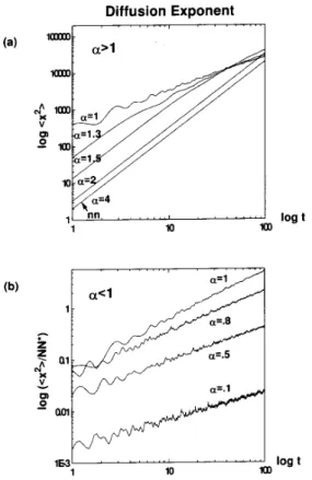
these curves is equal to, and we see that we have su-perdiusive properties in this regime. The slopes of the curves vary from=:9 (which appears to go to normal diusion of= 1 asN !1) for= 1 to= 2 (ballis-tic motion). Actually, all the curves for>1 start out with slope 2 for small times, but for 1:5 this time regime seems to dominate until nite size eects start entering, yielding= 2 for1:5. In Fig. 7b we show the normalized data<x
2
>=(NN
) for dierent values of1. For= 0 (not shown) the electron os-cillates on the lattice but on the average is trapped and therefore does not diuse at all. For=:1, we found that:5, which is clearly subdiusive behaviour. As increases so does , reaching the value = :9 1 (normal diusion) for= 1.
Figure 7: a) Log-log plots of < x 2
> versus time (units
of ~=V) are shown for dierent values of 1. Curves
are calculated usingN = 800. The slope of these curves is
equal to the diusion exponent , which varies from = 1
to= 2 in this regime. Note that all the curves for>1
seem to start out with slope 2 for small times. Only
for1:5 does this time regime seem to dominate until
-nite size eects become apparent. b) The renormalized data
<x 2
>=(NN
) is plotted versus time for dierent
1
using N = 800. The slopes shown here vary from :5
A summary of all of the above results is presented in Table I and in Fig. 8, where we show both and the constant C as a function of . Fig. 8a shows varying from :5 to 2 as a function of . In Fig. 8b the-dependent diusion constantCis shown for the region1 where the diusion coecient behaves as D = NN
C. For 1 < 2 the diusion goes as D = CN
() with
() shown in Fig. 6 andC as shown in Fig. 8c. The constantCaquires a maximum value at = 1:5. As of2 we obtainD=C, and C (shown in Fig. 8c) reaches the asymptotic value C= 2 for all4.
V Summary and Conclusions
In this paper we have studied the consequences of long-range interactions in a quantum mechanical tight-binding model of electrons on a one dimensional lattice. A hopping term proportional to 1=rij was used, where rij denotes the distance between atoms i and j and determines the range of the interactions within the system. Both thermodynamic and diusive properties were studied, as a function of the range of the inter-actions and of the system size. We found that only the minimum energy level Emin diverges as crosses over from the classically extensive regime ( >1 ) to the classically nonextensive regime ( <1). Further-more we were able to determine that this divergence is such that Emin=N
remains nite and constant for each < 1, with N
given by Eq (1). This makes sense because, for 1, N
is proportional to the number of particles interacting with each other, and the energy eigenvalue which diverges is one which con-sists of constructive contributions from all interacting atoms. All other eigenvalues remain nite because they contain both constructive and destructive contributions
due to the dierent phase factors associated with the dierent atoms.
Macroscopic thermodynamic quantities such as the internal energy and specic heat were calculated as a function of temperature and system sizeN. Somewhat surprisingly, they both appeared to be extensivefor all values of, showing no dependency onN
despite the divergence of Emin for<1. This can be understood as a consequence of the fact that the diverging state is essentially always occupied. This implies, for exam-ple, that the specic heat can only depend on the other energy levels, which are all nite and well-behaved for all values of. Our results are very dierent from the classical case where, for instance, the internal energy is predicted to scale as NN
. This dierence is probably due to the fact that in most classical settings we would expect all energies to scale as E=(NN
) [16] and not just one as E=N
.
We then studied the diusion of an electron along the lattice, and found large dierences in behaviour de-pending on the value of . These are summarized in Table I and in Fig. 8. We report here, for the rst time to our knowledge, that the diusion coecient diverges as D = CNN
in the regime
<1, where C is an -dependent constant. Furthermore, the diusion in this regime ranges from subdiusive (<1) to normal ( =:91), and exhibits high frequency oscillations. The behaviour changes at the critical value of = 1, after which there is superdiusion (1 < 2). The value of = 2, which corresponds to ballistic motion, is reached already for= 1:5. In addition, the scaling of the diusion coecent undergoes a transition from size-dependent to size-independent asgoes from 1 to 2. For 2,D is completely independent of the sys-tem size.
Table I -hx 2
i(t) =D t D and as a function of
D
= 0 (mf) D= 0 no diusion
0<<1 D=CNN
:5<1 subdiusion
= 1 D=CNlnN 1 normal diusion
1<<2 D=CN () 1
2 superdiusion
2 D=C = 2 ballistic motion
!1 (nn) D=C = 2 ballistic motion
0.0 0.2 0.4 0.6 0.8 1.0 0.00
0.02 0.04 0.06 0.08 0.10
0 1 2 3 4 0.0
0.5 1.0 1.5 2.0
1 2 3 4 5 0
1 2 3 4
5 α > 2
D=CαG(α)
c)
b)
a)
D=Cα 1 < α < 2
Cα
α
α <= 1 D=CαNN*
<x2>=Dtγ
Cα
γ
α α
Figure 8. a) The diusion exponent is shown here as a
function of the parameter , which determines the range
of the interactions. For 0 < 1 there is subdiusion
withranging from=:5 for smallalmost up to normal
diusion with = :9 for = 1. The regime > 1
ex-hibits superdiusive behaviour >1, approaching ballistic
motion= 2 at1:5 and beyond. b) For1 the
diu-sion coecientDis size-dependent such thatD=NN
C .
Here, we show howCvaries. c) For 1<2 the diusion
goes as D=CN
() with
() shown in Fig. 6 and C
as shown here. A maximum is obtained at= 1:5. As of 2 we obtainD=C
. C
reaches the asymptotic value
2 at about= 4.
These results deserve a little more discussion. In particular it is interesting to note the existence of three regimes of behaviour. This is analogous to results found for one-dimensional classical spin-systems [2], where there is a crossover from nonextensive to extensive be-haviour at= 1, yet there are two behavioural regimes within the extensive >1 parameter region. One of these is for 1 < < 2 and the other is for 2, which coincides with our results found here. This exis-tence of two distinct extensive regimes is a phenomenon only seen in one-dimensional systems. However, in the present quantum case, it may be that the real crossover from nonextensive to extensive behavior occurs at a value dierent from that in the classical case, because the behavior in the 1 < < 2 regime shows some
nonextensive scaling eects. Our work indicates that the quantum crossover may therefore be foras large as=d+ 1 = 2.
Another interesting point which is as yet unclear is why the diusion coecient diverges with NN
for 1. This may be related to the fact that we are considering the diusion of a single electron on the lat-tice, so that the lowest diverging energy level is likely to have a large inuence. The transition from subdif-fusive to superdiusive behaviour as we pass from the nonextensive to the classically extensive regimes is also not understood. However, both of these eects clearly must be investigated in greater detail.
In summary, we may say that the range of the hop-ping has considerable consequences for one-dimensional tight-binding systems. Though the thermodynamic properties of specic heat and internal energy appear largely unaected with respect to their extensive be-haviour, the diusive properties change drastically. It would surely be interesting to explore the behaviour of even more quantities for this simple system, and also to study the eects of long-range interactions in other quantum mechanical models.
Acknowledgements
The authors wish to thank Constantino Tsallis for initiating and inspiring this work through many help-ful discussions. JGM acknowledges nancial support from the Brazilian funding agency CNPq. LB acknowl-edges that this material is based upon work supported by the National Science Foundation under Grant No. INT-9703649. Infrastructural benets froma PRONEX grant (Brazilian agency) are also acknowledged.
References
[1] P. Jund, S.G. Kim and C. Tsallis, Phys. Rev. B52, 50
(1995).
[2] S.A. Cannas and F.A. Tamarit, Phys. Rev. B 54,
R12661 (1996).
[3] C. Anteneodo and C. Tsallis, Phys. Rev. Lett.80, 5313
(1998).
[4] C. Tsallis, J. Stat. Phys. 52, 479 (1988); E.M.F.
Cu-rado and C. Tsallis, J. Phys. A24, L69 (1991).
[5] A.R. Plastino and A. Plastino, Phys. Lett. A174, 384
(1993).
[6] B.M. Boghosian, Phys. Rev. E53, 4754 (1996).
[8] U.M.S. Costa, M.L. Lyra, A.R. Plastino and C. Tsallis, Phys. Rev. E26, 245 (1997); M.L. Lyra and C. Tsallis,
Phys. Rev. Lett.80, 53 (1998).
[9] P.A. Alemany and D.H. Zanette, Phys. Rev. E 49,
R956 (1994); D.H. Zanette and P.A. Alemany, Phys. Rev. Lett. 75, 366 (1995); C. Tsallis, S.V.F. Levy,
A.M.C. Souza and R. Maynard, Phys. Rev. Lett.75,
3589 (1995) [Erratum: Phys. Rev. Lett. 27, 5442
(1996)].
[10] A.R.Plastino and A.Plastino, Physica A 222, 347
(1995); C. Tsallis and D.J. Bukman, Phys. Rev. E
54, R2197 (1996); L. Borland, Phys. Rev. E57, 6634
(1998).
[11] L. Borland, J.G. Menchero and C. Tsallis Anoma-lous diusion and nonextensive scaling in a
one-dimensional quantum model with long-range
interac-tions, unpublished (1998).
[12] J.C. Cressoni and M.L. Lyra,The nature of electronic states in a disordered chain with long-ranged hopping
amplitudes, Physica A, in press.
[13] H.N. Nazareno and P.E. de Brito Long-range
interac-tions and nonextensivity in one-dimensional systems,
Preprint (1998).
[14] P.W. Anderson and G. Yuval, Phys. Rev. B 1, 1522
(1970);
[15] D.J. Amit, Modeling Brain Functions, (Cambridge University Press, 1989).