A review on sequential injection methods for water analysis

A review on sequential injection methods for water analysis

Raquel B.R. Mesquita, António O.S.S. Rangel

CBQF/Escola Superior de Biotecnologia, Universidade Católica Portuguesa, R. Dr. António Bernardino de Almeida, 4200-072 Porto, Portugal

Keywords: Sequential injection Lab-on-valve Bead injection Water analysis Review

a b s t r a c t

The development of fast, automatic and less expensive methods of analysis has always been the main aim of flow methodologies. The search for new procedures that still maintain the reliability and accuracy of the reference procedures is an ever growing challenge. New requirements are continually added to analytical methodologies, such as lower consumption of samples and reagents, miniaturisation and portability of the equipment, computer interfaces for full decision systems and so on. Therefore, the development of flow methodologies meeting the extra requirements of water analysis is a challenging work.

Sequential injection analysis (SIA) presents a set of characteristics that make it highly suitable for water analysis. With sequential injection analysis, most routine determinations in waters can be per-formed more quickly with much lower reagent consumption when compared to reference procedures. Additionally, SIA can be a valuable tool for analyte speciation and multiparametric analysis. This paper critically reviews the overall work in this area.

∗ Corresponding author. Tel.: +351 225580064; fax: +351 225090351.

E-mail address:aorangel@esb.ucp.pt(A.O.S.S. Rangel).

Water is an essential resource that is being threatened by pol-lution; therefore, the monitoring of water quality has become an issue of vital importance. The European Union has created the Water Framework Directive (WFD) in order to improve, protect and

Introduction

prevent further deterioration of water quality across Europe[1]. Accurate and frequent monitoring of water quality enables tighter control of the governmental regulations which is an important step in the reduction of the water pollution. It is estimated that, in Euro-pean surface waters, the impact of pollution caused by industrial discharges of toxic substances has decreased 70% over the past 30 years[2]. This reduction has resulted from the implementation of stricter governmental regulations as much as the development of cleaner technologies.

The term “water” used in WFD includes most types of water, i.e. ground, surface and coastal waters. Several “water quality ele-ments” are covered such as:

• Physicochemical properties – temperature, density, colour, tur-bidity, pH value, redox potential, conductivity, surface tension, suspended solids, total/dissolved organic carbon;

• Hydromorphological status – erosion and bench river character-istics;

• Biological – distribution and composition of the species and bio-logical effects;

• Chemical monitoring – with particular emphasis on the contam-inants in the list of priority pollutants.

Changes in water composition can be an indicator of pollu-tion or contaminapollu-tion, so frequent water analysis is imperative. Some parameters are under strict regulation because of their risk to human health while others are not subject to enforceable regula-tion as they only cause visual or aesthetic effects[3]. More recently, the public concern for water safety has led to an increase on the use of disinfectants, which in turn has become a problem itself, if the carcinogenic by-products generated by the disinfectants are considered. Nevertheless, water disinfection is essential to ensure public health. Disinfectants prevent water contamination by bac-teria but if in excess are harmful to human health, both directly and through by-products. In the last Analytical Chemistry bien-nial review on water analysis[4], the importance of disinfectants and their by-products as new contaminants was highlighted. These biennial reviews are focused on emerging contaminants and trends of analytical developments concerning water analysis.

The monitoring of water quality relies on effective routine water analysis, so this became a hot, sensitive and trendy issue. The range of methods, processes and tools available can be classified in dif-ferent ways. A useful classification, revisited by Greenwood et al. [2], is based on the relationship between sample and analytical processes with three main categories: (i) in situ, (ii) on-line and (iii) off-line. Generally, the methods with no sampling, the meth-ods with in-situ determination, use sensing devices such as probes inserted directly in the water body. Regarding on-line methods, the determination is carried out close to the water being monitored with direct feeding into the analytical system. In those cases, both discrete and continuous flow measurements can be performed.

Some major challenges in water quality monitoring include: a wide range of analyte concentration; variable salinity (wide range of ionic strength); colour or turbidity (mainly in waste waters); spe-ciation; the need to mineralisation prior to quantifying the total amount. Analytes can be present in a high amount and so dilution may be necessary to fit the linear range, or they can be present in trace amounts and thus a preconcentration step is required. The variability in ionic strength may cause interferences in the chemistry itself or then influence the analytical signal, namely in spectrophotometric measurements. Water colour or turbidity may lead to high blank values which may adversely affect the limit of detection. The growing interest of environmental chemists in analyte speciation also poses an additional challenge, as some traditional methods only permit to quantify the total amount, namely when a reaction is used to quantify a certain analyte form

may induce equilibrium shifts that unable to quantify the exact amount in that form. The interest of environmental chemists in analyte speciation relies on the tight relationship between speci-ation, bioavailability and toxicity. For example, aluminium is only bioaccumulated by organisms in the form of Al3+_{. Organisms use}

nitrate as nitrogen source while the nitrite form is highly toxic. Fur-thermore, changes in the environment caused by pollution such as environmental acidification result in the release of the cationic form of several metals, their most bioavailable form. The impact to human health becomes a consequence of the environmental impact. With the sequential injection versatility, this issue of ana-lyte speciation can be tackled.

On the other hand, there are situations in which the quantifi-cation of the total amount is required and so drastic digestion conditions must be created. All these issues increase the complexity of water analysis.

In addition, the analysis of water should also try to comply with the objectives of so-called Green Chemistry[5], in order to reduce and/or eliminate the use and generation of hazardous substances. In fact, an ironic situation is created when the analytical method-ologies employed to monitor pollutants generate chemical wastes that are highly polluting themselves[5]. In some cases, the chemi-cals used in the analysis are even more toxic than the analyte itself, which makes the search of new alternatives even more pertinent.

In this scenario, flow systems may provide answer to the above mentioned challenges, as virtually every unit operation can be implemented in-line, and offer several advantages for routine anal-ysis namely, high sampling rate, miniaturisation, low sample and reagent consumption. The variety and capability of flow tech-niques and flow equipment has increased significantly over the last three decades. Scale of the equipment has gone from bench size equipment, handling volumes measured in liters, to coin size equip-ment with volumes in the order of microliters. This review focuses on the sequential injection analysis (SIA) approaches that meet some of these challenges, choosing sequential injection analysis [6]among the different automatic flow techniques (flow injection [7], multicommuted flow injection [8], multisyringe flow injec-tion[9], multipumping flow[10]). This choice was determined by the robustness of the equipment along with the compact size, the possibility of multiparametric determinations and the low reagent consumption. In addition, the easy coupling of external devices such as gas diffusion or dialysis units, resin packed columns and so on, enables the application to a wide variety of waters. These features result from the versatility of the sequential injection valve which enables a direct connection to the various reagents and/or to external devices.

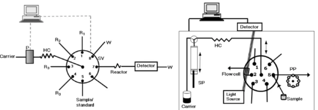
Sequential injection was proposed as an evolution to flow injec-tion analysis, to overcome some of its perceived disadvantages, the requirement for a separate manifold for the determination of each parameter and the continuous consumption of reagents. Other flow techniques such as multicommutation, multisyringe and multipumping overcome the continuous consumption of reagents but maintain, in many circumstances, the requirement of physical reconfiguration for different methodologies. Sequential injection has the ability of performing different determinations without sys-tem reconfiguration (placing different reagents on the ports of the selection valve) and there can be a reagent saving associated to non-continuous consumption. In a SIA manifold (Fig. 1(I)), sample and reagent solutions are sequentially aspirated into a holding coil, being the aspirated volumes determined by the time and aspiration

Sequential injection analysis

Fig. 1. Sequential injection manifolds: (I) conventional manifold of sequential injection: SV – selection valve, P – propulsion device, HC – holding coil, Ri – reagents, W – waste; (II) sequential injection lab-on-valve manifold: HC – holding coil, PP – peristaltic pump, SP – syringe pump.

rate; the mutual mixture is promoted by flow reversal, while send-ing the stacked zones towards the detection system. The computer control ensures the reproducibility of the process.

The basic components of sequential injection are schematically represented inFig. 1(I). The key equipment is the multi-port selec-tion valve as it enables the sequential selecselec-tion of the various solutions and the subsequent redirection towards the detection sys-tem. Most of the characteristics attributed to sequential injection are due to the selection valve. In fact, the placement of different reagents on the ports permits different determinations with the same manifold and it is the structure of the selection valve itself that gives robustness to the sequential injection technique. The sequen-tial aspiration of reagent and sample is made possible through the presence of the holding coil which prevents the contamination of the carrier. The propulsion system is usually a peristaltic pump or a piston pump and different detection systems can be used.

A step forward in miniaturisation and compaction of the sequen-tial injection concept was recently achieved with micro sequensequen-tial injection lab-on-valve (SI-LOV) equipment[11]. The SI-LOV con-cept was described as a universal micro-flow analyser based on the sequential injection concept. It resulted from the incorpora-tion of the detecincorpora-tion system in the selecincorpora-tion valve which was made possible due to the use of fibre optics technology. With this sig-nificant down scale of sequential injection, there is an even lower consumption of reagents and samples. The micro sequential injec-tion lab-on-valve concept is considered the third generainjec-tion of flow analysis.

All the equipment, i.e. selection valve, propulsion device and detector, are assembled in the same box (Fig. 1(II)) resulting in the most compact of all the flow methodologies. As mentioned above, the volumes used are extremely small and the flow cell is posi-tioned on the valve, which makes the analytical path rather short. The advantages in reagent and sample consumption minimisation are obvious and make SI-LOV a perfect tool for enzymatic and the so-called bead injection assays. The bead injection technique can be considered a “hyphenated” technique as it is commonly cou-pled with some other fluidic handling technique[12], where beads replace the reagent solution and the assay is carried on in the beads surface. This technique is especially suitable for immunoassays, coating the beads with antibodies.

The features of simplicity and versatility allied with robust-ness have created an exponential growth of SIA applications. This growth in publications since SIA was first described in 1990, results not only from the relatively simple implementation but also the wide applicability of sequential injection techniques. From 1990,

the cumulative number of papers increased to 286 in 2000, reach-ing 1204 papers last year (calculated usreach-ing ISI Web of Knowledge – Web of Science, keyword “sequential injection”, 19/01/2009). The increase in SIA publications numbers is not, however compara-ble to flow injection and one of the reasons for that could be the requirement of computer control. This requirement implies some knowledge in computing for writing the programs as well as inter-facing of the equipment used, which may be complex. Another reason could be the parallel development of other flow techniques (mentioned above) that have emerged from the original main con-cept of flow injection.

Along with all this increase in the diversity of flow manipulation, the possibilities in detection systems have also evolved extraordi-narily. This evolution was not only in diversity but also in size, while fluid volumes have been reduced from mililiters to microliters and spectrophotometers have decreased in size about 80 fold. Therefore, the combination of flow handling techniques and detection systems has led to a countless number of possibilities. This may be the rea-son why there has also been an increase in the range of applications. Nowadays, flow systems have been developed for nearly all types of samples ranging from pharmaceutical preparations to complex solid samples such as soil and food. Based on the previously ISI Web of Knowledge – Web of Science search (Fig. 2) of sequential injec-tion publicainjec-tions, a cross linked search with possible samples or types of sample enabled some conclusions to be drawn regarding the application of the described sequential injection systems.

First the types of sample were broadly categorized on environ-mental, food, pharmaceuticals or biological. Then, more specific classifications were used: wine, milk, water, plant extracts, soils and slurry. It is quite obvious that some overlap occurred as for example wine and milk are included in “food”, and water and soil are included in “environmental”, but the idea was to be as thorough as possible. “Biological samples” is the term commonly

Fig. 2. Schematic representation of a SIA manifold for the multiparametric determi-nation of calcium, magnesium and alkalinity in natural waters (adapted from[78]): P – peristaltic pump, BG – bromocresol green reagent for alkalinity determination, Q – hydroxiquinoline as masking agent for magnesium in calcium determination, EGTA – masking agent for calcium in magnesium determination, CPC – cresolphtalein complexone colour reagent for calcium and magnesium determination, S (alkalin-ity)/S (Ca, Mg) – sample for alkalinity or calcium and magnesium determination, respectively.

Micro SIA (SI-LOV) and bead injection (BI)

used for samples as urine, blood and serum. In the end, almost half of all the described publications were not included in any category. Nevertheless, water samples are one of the three most common applications of the sequential injection technique along with pharmaceutical preparations and biological samples. It is a quite significant percentage which illustrates the concern for automation of water monitoring, especially when the other two main applications are health related, to pharmaceuticals and bio-logical samples.

As far as we know, no previous review was dedicated solely to sequential injection for water analysis. A review by Cerdà et al.[13]was dedicated to sequential injection applied to environ-mental samples, which include water, plants and soils. The papers [9,14–16]describe different flow methods for analysing waters and [17,18]are dedicated to the application of flow injection to the same matrix.

In some reviews[19–21], the focus was on the evolution of flow methodologies, in which sequential injection was mentioned as a versatile and robust flow technique to couple with devices for in-line treatments. Other reviews have focused on new developments in detection systems coupled with flow techniques[22–25], namely sequential injection. Some reviews of specific detection methods such as vibrational spectroscopy [22], FTIR [23], electrothermal atomic absorption spectroscopy[24]and electronic tongues[25] emphasised the versatility of flow techniques, including sequential injection.

It is also worth mentioning reviews on the determination of specific parameters/analytes (nutrients in aquatic systems[26], phosphorus determination[27]), or a specific type of sample (sea water analysis[28]).

The applications of the sequential injection concept to water analysis are presented inTable 1. Molecular absorption spectrom-etry is by far the most commonly used detection method. This may be due to characteristics such as the robustness of the equipment, the possibility of miniaturisation, the versatility of application and the overall cost. Furthermore, it is a quite simple technique, not requiring any specific training. Other spectrophotometric detection systems such as flame emission atomic spectrometry (FEAS), flame atomic absorption spectrometry (FAAS), electrothermal atomic absorption spectrometry (ETAAS) and inductively coupled plasma mass spectrometry (ICP-MS) are generally more sensitive and selective, allowing trace elements analysis, but present a high main-tenance costs and are not easily miniaturised. In addition, a more specific training is normally required. In the case of fluorescence and luminescence, the miniaturisation and cost are no longer a problem but the applicability is highly restricted. As for detection systems based in electroanalytical techniques such as potentiome-try, amperometry and voltammepotentiome-try, the portability and the in-situ determination are the main advantages. The problem with these techniques might be robustness and in some cases the limits of quantification.

One of the most common drawbacks attributed to sequential injection methods is the lower determination rate, especially when compared to flow injection. Nevertheless, that depends entirely on the method itself as it can be observed inTable 1.

There is an extremely wide range of determination rates; from 3 determinations per hour in a methodology including separation and preconcentration[118]to 189 determinations per hour in a multiparametric determination[83]. The easy implementation of multiparametric determinations and diverse in-line sample treat-ments is a key attribute of sequential injection systems.

More than 45% of the methods listed inTable 1were applied to more than one type of water and 12% were applied to more than two types. This emphasises the versatility of sequential injection which can be applied to different types of water samples, by minor mod-ifications in the flow programming, without any physical change of the manifold. Actually, some observations can be pointed out: (i) the significant percentage (over 6%) of papers that did not spec-ify the sample used; (ii) the percentage of papers that classified the sample as “natural water”, close to 11%, which include several types of water (sea, rain, river, lake, ground, mineral and tap water); and (iii) the percentage of papers that classified the sample as “sur-face water”, close to 5%, which also includes several types of water (sea, mineral river and lake). Tap water and waste water were the most analysed types with about 15% each of the listed papers. Rain [118]and mine[136]waters were the least analysed, with only one methodology applied to each one.

One of the main advantages of sequential injection analy-sis is its potential to perform multiparametric analyses. This means that by using the same manifold but placing different reagents on the selection valve ports, and changing the operational parameters, more than one analyte can be determined. From the listed papers, over 40% involved the determination of more than one analyte[34–36,39,40,45,49–53,55,59–61,72,74,78,83–85, 94,96,101–104,106,107,114,116,117,119,120,132,135,138,140,141,145, 148,149,153,155], with close to 18% describing the determination of more than two analytes[34–36,40,45,49–51,53,74,83,78,102,101, 116,140]. Some more detailed examples of bi-parametric determi-nations will be detailed in Section3.4.2, as they usually involve quantifying two oxidation states. When more than two analytes are considered, it usually implies the coupling to multi-analyte detection systems like ICP, HPLC or an array of sensors. This multiparametric capacity minimises the disadvantage of a low sample throughput that is often attributed to SIA. An example of a multiparametric SIA system with a determination rate of 40 h−1for two parameters (calcium and magnesium) and 65 h−1for a third one (alkalinity) is illustrated inFig. 2.

Another mentioned advantage of sequential injection is the ease coupling of separation devices to the valve, without overall man-ifold reconfiguration. This feature is due to the use of a selection valve, enabling the direct connection to the separation device. In fact, about 45% of all the listed papers described an in-line treat-ment of the sample. Within these papers, different types of in-line treatment are considered, some aiming for the separation and/or preconcentration of the analyte (_{≈70%) and others aiming for the} change of the oxidation state of the analyte (≈30%).

Most of the works that include preconcentration and/or separation of the analyte refer to coupling SI methodology with ICP[50,51,58,102]and AAS[38,39,41,47,48,56,72,73,90,99,100, 113,114,126,129,143]. The combination of SIA with ICP or AAS asso-ciates the advantages of SIA such as versatility, robustness and automation (useful for handling reagent and sample preparation) with selectivity and sensitivity of those detection methods. The problems that normally arise from using a complex matrix were avoided by appropriate sample preparation, namely the inclusion of a preconcentration step; additionally, limits of detection of 1 pg L−1 were obtained[50].

Water analysis using SIA

Water samples

Multiparametric determinations

In-line treatments

Table 1

Sequential injection systems for water analysis.

Year Analyte Sample Detection system Determination conditions Dynamic range LOD RSD Determination

rate

Ref.

2008 Methyl parathion Surface water Voltammetry SI for in-line sample

conditioning and standard addition

0.010–0.50 mg L−1 0.002 mg L−1 <4.5% 25–61 h−1 [29

2008 Linear alkylbenzene sulfonates

Natural water Spectrophotometry/

chromatography

Lab-on-valve approach used for application of two detection methods

0.07–10␮g L−1 21 ng L−1, <10.2% 36–29 h−1 [30]

15␮g L−1

2008 Nitrite Seawater Spectrophotometry Griess reaction with solid phase enrichment of the coloured product prior to detection

0.71–42.9 nM and 35.7–429 nM

0.1 nM 1.44% 4 h−1 [31]

2008 Fluoride Natural water Potentiometry Comparison between a SI system and a flow injection system for the application of a tubular electrode

0.5–6.0 mg L−1 0.1 mg L−1 4% 30 h−1 [32]

2008 Phosphorus Sea water Spectrophotometry Solid phase extraction with a hydrophilic–lipophilic balance used to enrich phosphomolybdenium blue

3.4–1132 nmol L−1 1.4 nmol L−1 2.5% 6–10 h−1 [33]

2008 Na, K and chloride Mineral water Potentiometry SI system with integrated multisensor chip as base for “electronic tongue”

0.05 mM–0.01 M – <8% – [34]

2008 Mg, Ca, Na and K Synthetic water Potentiometry SI for automate the training of the “electronic tongue” employing the pulse transient response

– – – – [35]

2008 Na, K and chloride Mineral water Potentiometry SI system based on a multisensory ISFET array monolithically integrated in one chip

– – – – [36]

2008 Al Natural and waste water Spectrophotometry A direct and kinetic determination based in the reaction with chrome azurol S

0.040–0.500 mg L−1 _{0.002 mg L}−1, 0.012 mg L−1 <5%, <9%

57 h−1 [37]

0.05–0.300 mg L−1 31 h−1

2008 Cr(III) and Cr(VI) Certified river water and cave water

Electrothermal atomic absorption spectrometry

Chromium speciation by bio-sorption of Cr(VI) on egg-shell membrane, Cr(III) obtained by subtraction (after conversion to Cr(VI)

0.05–1.25␮g L−1_{Cr(VI) 0.01␮g L}−1_{Cr(VI) 3.2% 15 h}−1 _[38]

2008 Cr(VI) and Cr(III) River and tap water Electrothermal atomic absorption spectrometry

Preconcentration and speciation of chromium using two mini-columns

0.1–0.25␮g L−1Cr(III), 0.12–2.0␮g L−1Cr(VI) 0.02 Cr(III), 0.03 Cr(VI) (␮g L−1) 1.9% Cr(III), 2.5% Cr(VI) 10 h−1 [39]

2008 Pb, Cd and Zn Certified river water Voltammetry Anodic stripping

voltammetry with a bismuth film screen-printed carbon electrode 0–70␮g L−1Pb e Cd, 0.075–0.200␮g L−1Zn 0.89␮g Pb L−1, 0.69␮g Cd L−1 <8.8% – [40]

2008 Pb(II) Natural water Flame atomic absorption spectrometry Liquid–liquid micro-extraction for preconcentration and/or separation 3.0–250.0␮g L−1 1.4␮g L−1 2.9% 25 h−1 [41] 2007 Alkylphenol polyethoxylates

River water Chemiluminescence Immunoassay with microbeads

0–1000␮g L−1 _{10␮g L}−1 _{– 4 h}−1 _[42]

2007 Picloram River and tap water Squarewave voltammetry Mercury drop electrode 0.1–2.5 mg L−1 36␮g L−1 10.0% 37 h−1 [43]

2007 Chlorine Surface and tap water Spectrophotometry Direct determination with as a new application of tetramethylbenzidine

Table 1 (Continued )

Year Analyte Sample Detection system Determination conditions Dynamic range LOD RSD Determination

rate

Ref.

2007 Mg, Ca, Ba Mineral water Potentiometry Electronic tongue,

PVC-membrane

potentiometric sensor array and multivariate calibration

0–120 mg Ca L−1 – – – [45]

2007 Hg Certified river water and sea water

Atomic fluorescence spectrometry

Lab-on-valve approach with a micro-scale vapor generation chamber

0.06–10␮g L−1 0.02␮g L−1 4.4% 90 h−1 [46]

2007 Cd Lake water and certified river water

Electrothermal atomic absorption spectrometry

Use of cell-sorption for separation/preconcentration

0.005–0.2␮g L−1 _{1.0 ng L}−1 _{2.3% 20 h}−1 _[47]

2007 Cu Coastal seawater and certified seawater

Electrothermal atomic absorption spectrometry

Sequential injection used for sample pre-treatment and concentration

0.05–1.00␮g L−1 _{0.015␮g L}−1 1.8% 26 h−1 [48]

2007 Co, Ni, Cu, Fe Drinking waters HPLC/spectrophotometry SI for automated handling of sample/reagents, on-line pre-column derivatization and propulsion to HPLC From 5–75␮g L−1to 7–1000␮g L−1 From 1␮g L −1to 2␮g L−1 6.0% 4 h −1 [49] 2007 Be, Cd, Cr, Cu Pb and other metals

Certified river water and tap water

ICP-MS or ICP-AES SI for sample preparation and pre-treatment From 0.001–10 ng L−1to 0.1–10 ng L−1 From 0.001 ng L−1to 018 ng L−1 9.6% 11 h−1 [50]

2007 Ag, Be, Cd, Co, Cu, Ni, Pb, U, V

River water ICP-MS Preconcentration of trace elements From 0.005–5␮g L−1to 1–5␮g L−1 From 0.001␮g L −1to 0.93␮g L−1 From 0.2% to1.2% – [51]

2006 Ammonia phosphate River and marine water Fluorimetry Free reactive phosphate detected by suppression of rhodamine fluorescence by phosphomolybdate and ammonia with phthaldehyde

0.02–20␮M 0.02␮M –

120 h−1 [52]

0.04–4␮M 0.04␮M

2006 Chloride, nitrate, hydrogencarbonate

Well, spring and tap water

Potentiometry Array of potentiometric sensors and artificial neural network, “electronic tongue”

– – <7% – [53]

2006 Pharmaceutical compounds

Surface water and raw and treated waste waters

HPLC/spectrophotometry Lab-on-valve as a front end to HPLC with on-line solid phase extraction

– 0.05␮g L−1 – – [54]

2006 As(III) and As(V) Tap water and groundwater

Chemiluminescence SI for fluidic handling for measure waterborne arsenic

0–50␮g L−1 _{0.05␮g L}−1 _{– 15 h}−1 _[55]

2006 Ni Tap and seawater Electrothermal atomic absorption spectrometry

Bead injection for separation/preconcentration

0.2–2␮g L−1 0.05␮g L−1 4.8% 10 h−1 [56]

2006 Se River, lake and tap water AAS-Hybrid SI for handling sample/reagent

0.10–8.0␮g L−1 0.03␮g L−1 2.8% 24 h−1 [57]

2006 Pb Reference river water & river samples

ICP-MS Preconcentration resin Vs = 5 0.1–5 ng mL−1 70 pg mL−1 0.5% 12 h−1 [58]

Preconcentration resin Vs = 10

30 pg mL−1

2006 Cu(II) Standard solution and industrial waste water

Spectrophotometry LOV, use of reducing agent for determination of iron(II)

0.1–2 mg L−1 50␮g L−1 2.0% _{18 h}−1 [59]

Fe 0.1–5 mg L−1 25␮g L−1 _1.8%

2006 Cr(VI) Simulated water samples Spectrophotometry–diode array

Chemometric tools-multivariate curve resolution alternative least squares (MCR-ALS)

0.02–0.5 mg L−1 2.4␮g L−1 _{3.7% 54 h−1 [60]}

Cr(III) – – 4.9%

2006 Cr(VI) Simulated water samples Renewable surface reflection spectrophotometry

Reaction with Cr(IV) in beads and oxidation of Cr(III) to Cr(IV)

0.02–0.5 mg L−1 2.4␮g L−1 1.3% _{53 h}−1 [61]

Cr(III) – – 2.5%

2005 3,5,6-trichloro-2-pyridinol

Tap water and river water

Electrochemical immunoassay

Magnetic beads coated with antibody in a permanent magnet reaction zone

0.01–2␮g L−1 6 ng L−1 <3.9% - [62]

2005 Cationic surfactants Well and tap water Spectrophotometry Reaction of cationic surfactants as zephiramine among others with bromophenol blue

2005 Cationic surfactants Surface and waste waters Spectrophotometry Different colour reagents for each determination

8.10−6to 1.10−4M, 1.10−4to 5.10−4M

2.20.10−6M, 2.96.10−4M 4.57%, 4.93% 29 h−1, 28 h−1 [64]

2005 Anionic surfactant Drainage water sample Spectrophotometry Liquid–liquid extraction, lab at valve approach

1–10 mg L−1 0.48 mg L−1 5.0% 5 h−1 [65]

2005 p-Arsenilic acid

(p-ASA)

Surface water from swine farm

Spectrophotometry Sequential injection-long path length absorbance spectrometry (SI-LPAS)

0.1–1.0 mg L−1 0.0212 mg L−1 2.8% 7.5 h−1 [66]

2005 Nitrite Waste water treatment plant Spectrophotometry Adaptative system for 2 ranges, automatically programmable

0.0–3.0 mg L−1 0.048 mg L−1 – 12 h−1 [67]

0.0–20.0 mg L−1 0.4 mg L−1

2005 Atrazine Waste and fresh water Square wave voltammetry SI for conditioning and standard addition

1.2× 10−7M to 2.3× 10−6M

2.1× 10−6M 5.2% 37 h−1 [68]

2005 Chlorine Tap water, waste water and bleaches

Spectrophotometry Gas diffusion unit for separation of free chloride, colorimetric detection

0.6–4.8 mg L−1 0.5 mg L−1 2.0% 15 h−1 [69]

0.047–0.188 g L−1 5 mg L−1 2.0% 30 h−1

2005 Chloride Mineral drinking water and surface water

Potentiometry Lab-at-valve approach with the electrodes attached to the multiposition valve

0.10–120 mM – 1.3% 50 h−1 [70]

2005 Fe(III) Not specified water samples

Spectrophotometry Home-made SIA, Fe–thiocyanate complex

1.0–7.0 mg L−1 0.34 mg L−1 1.1% – [71]

2005 Cr(VI) River, lake and tap water Electrothermal atomic absorption spectrometry

Bead injection for separation/preconcentration

0.035–0.4␮g L−1 _{0.02␮g L}−1 _{2.2% 8 h}−1 _[72]

Cr(III) 0.02–0.25␮g L−1 _{0.01␮g L}−1 2.4% 12 h−1

2005 Cr(VI) Seawater, tap water and certified natural water

Electrothermal atomic absorption spectrometry

Bead injection with renewable reverse phase for separation/preconcentration

0.12–1.5␮g L−1 0.03␮g L−1 3.8% 15 h−1 [73]

2005 Cu, Fe, Mn, Zn Natural, waste and spiked water samples

Spectrophotometry Different colour reagents for each determination 0–5 mg L−1, 0–10 mg L−1, 0–4 mg L−1, 0–5 mg L−1 0.048 mg L−1, 0.012 mg L−1, 0.24 mg L−1, 0.013 mg L−1 2.4%, 2.8%, 2.1%, 2% – [74]

2004 Bromate Not specified water samples

Spectrophotometry Reaction between bromate and PADAP with thiocyanate

0.18–3.00 mg L−1 0.15 mg L−1 0.8% 45 h−1 [75]

2004 Boron Natural waters and pharmaceuticals

Fluorimetry Calibration curve based in boric acid and related to boron

8–350 mg L−1 0.003 mg L−1 2.7% 49 h−1 [76]

2004 Orthophosphate Waste water treatment plant

Spectrophotometry On-line electrochemical generation of molybdenum blue

0.3–20 mg L−1P 0.100 mg L−1P 2.4% 18 h−1 [77]

2004 Ca, Mg Drinking, surface, tap water and reference water

Spectrophotometry Same reagent for Ca and Mg (cresolftaleine) with masking agents, alkalinity with bromocresol green 0.5–5 mg Ca L−1, 0.5–10 mg Mg L−1 0.32 mg Ca L−1, 0.03 mg Mg L−1 2.0% Ca, 2.1% Mg 40 + 40 h−1 [78]

Alkalinity 10–100 mg L−1HCO3− 5.1 mg L−1HCO3− 0.4% 65 h−1

2004 Al Drinking water during and after

flocculation/coagulation

Fluorimetry Separation of Al from matrix with XAD-4 (chelating resin) reaction with

hydroxyquinoline

0.2–500 mg L−1 0.2 mg L−1(mL−1 sample)

– – [79]

2004 Hg River and sea water Cold-vapour atomic absorption spectrometry

Inclusion of a new integrated gas–liquid separator operating in parallel as a reactor

0.05–5␮g L−1 0.02␮g L−1 2.6% 25 h−1 [80]

2004 Pb Natural and waste water Spectrophotometry Preconcentration of Pb in Chelex and interferences removal in AG1X8 (resins)

0.05–0.30 mg L−1 25␮g L−1 _{3.6% 17 h}−1 _[81]

0.30–1.0 mg L−1 165␮g L−1 1.0% 24 h−1

2004 Pb Drinking water samples Spectrophotometry Catalytic effect on reaction with reazurin

0–0.100 mg – 3.0% – [82]

2004 Pb, Zn, Co, Cd, Cu, Fe(III), Hg

Soils, tap waters, urine and certified samples

Spectrophotometry–diode array

Thin-film SI extraction with multivariate calibration and multiwavelength detection 1–20 Co, Cu, Pb, 1–10 Hg, 1–20 Zn, 1–20 Cd (mg L−1) – 2.0% 27 h−1 (189 dt h−1) [83]

Table 1 (Continued )

Year Analyte Sample Detection system Determination conditions Dynamic range LOD RSD Determination

rate

Ref. 2003 Carbonate and

hydrogencarbonate

Not specified water samples

Spectrophotometry Titration using

phenolphthalein and methyl orange 0.8–10 mM CO32−, 1–10 mM HCO3− – 2% CO32−, 1.5% HCO3− 12 h−1 [84]

2003 Bromine Spiked water samples and effluents streams

Spectrophotometry Determination of bromine and total bromine, oxidation, (bromide by the difference)

1–10 mg L−1Br2 0.6 mg L−1Br2 0.8% Br2 30 h−1 [85]

Bromide 0.8–15 mg L−1total Br2 0.4 mg L−1total Br2 0.7% total Br2

2003 sulphate Natural and waste waters

Spectrophotometry Use of an air bubble for minimise dispersion and improve mixing, turbid metric determination (BaCl)

10–100 mg L−1 10 mg L−1 5% 20 h−1 [86]

2003 Sulphide Simulated water samples Spectrophotometry Based in formation of methylene blue dye, calibration with in-line dilution of a single standard

0.17–1.0 mg L−1 0.04 mg L−1 5.20% 38 h−1 [87]

2003 Tween-80 Well water, tap water and seawater all spiked

Fluorimetry Enhancement of fluorescein fluorescence in the presence of Tween-80

10–2100␮g L−1 _{1.7␮g L}−1 _{2.70% – [88]}

2003 Al Tap water spiked Fluorimetry Enhancement of the fluorescence of the complex aluminium–morin with Tween-20

50–1000␮g L−1 3␮g L−1 2.90% – [89]

2003 Cd Reference river and natural water

Electrothermal atomic absorption spectrometry

Coupling bead injection with lab-on-valve for on-line matrix removal and preconcentration

0.05–1␮g L−1 15 ng L−1 3.10% 12 h−1 [90]

2003 Cr(VI) River and lake water samples

Spectrophotometry Comparative studies of diffusion samplers using diphenylcarbazide (DPC)

0–1.6 mg L−1(without membrane)

20 mg L−1 1.10% – [91]

2003 Cu Mineral and tap water Spectrophotometry Reaction with cuprizone, sandwich SIA compared to FIA

0.06–4 mg L−1 0.004 mg L−1 0.71% 48 h−1 [92]

2003 Hg (total) River water samples spiked

Spectrophotometry Bead injection with Chelex resin and dithizone for colorimetric reaction

0–30 mg L−1 0.9 mg L−1 9% 20 h−1 [93]

2003 Mn(II) River water samples and effluents streams

Spectrophotometry Determination of Mn(II) and total Mn (Mn(VII) by the difference)

0.02–0.50 mg L−1Mn(II) 0.005 mg L−1Mn(II) 0.27% Mn(II) 30 h−1 [94]

Mn(VII) 0.025–0.55 mg L−1total

Mn

0.008 mg L−1total Mn 0.34% total Mn 2002 Chloride Ground, surface and

waste water

Spectrophotometry Turbidimetric determination based in the reaction between silver nitrate and chloride

2–400 mg L−1 2 mg L−1 3.7% 55 h−1 [95]

2002 Nitrite nitrate Surface water Spectrophotometry Direct determination of nitrite, reduction of nitrate to nitrite in a

copperised-cadmium column

0.05–1.00 mg N L−1 0.015 mg N L−1 1.10% 14 h−1 [96]

0.50–50.0 mg N L−1 0.10 mg N L−1 1.32%

2002 Fluorophores Tap and mineral water Variable angle scanning fluorescence spectrometry

Multicomponent mixtures coupling the detection with multivariate least squares regression From 0.05–5␮g L−1_to 13–720␮g L−1 From 0.02␮g L −1_to 10␮g L−1 <1.0% 17 h −1 _[97]

2002 Al Drinking and tap water Spectrofluorimetry Reaction between Al and hydroxyquinoline and fluorimetric detection of the complex

2002 Cd Natural waters Electrothermal atomic absorption spectrometry

SI for on-line solvent extraction-back extraction

0.05–0.8␮g L−1 2.7 ng L−1 1.8% 13 h−1 [99]

2002 Cd Natural waters Electrothermal atomic absorption spectrometry

SI for on-line matrix removal and preconcentration

0.02–0.2␮g L−1 1.2 ng L−1 1.5% 16 h−1 [100]

2002 Cd, Cu, Pb and Zn Drinking and waste waters

Voltammetry Comparison of between a flow injection system and a sequential injection system (still in study)

From 10–70␮g L−1to

470–700␮g L−1 From 6␮g L −1to

4700␮g L−1 <9.8% – [101]

2002 Al, As, Co, Cu, Mn, Mo, Ni, Pb and V

Sea water ICP-MS Comparison of different resins for preconcentration

0–100␮g L−1 – <5% – [102]

2002 Fe(III) Effluents streams Spectrophotometry Determination of Fe(III) and total Fe, oxidation, (Fe(II) by the difference)

0.15–100 mg L−1 0.10 mg L−1 1.3% Fe(III) _{30 h}−1 [103]

Fe(II) 0.30–80 mg L−1 0.15 mg L−1 0.8% Fe(II)

2002 Cr(III) Water samples (not specified)

Spectrophotometry Direct determination of Cr(VI) and total Cr (oxidation of Cr(III) to Cr(VI)), Cr(III) by the difference

0.85–25 mg L−1 0.042 mg L−1 0.70% 30 h−1 [104]

Cr(VI) 0.16–20 mg L−1 0.023 mg L−1

2002 90_{Sr Mineral, ground and}

marine water

Low-background gas-flow proportional counter

Si for on-line wetting-film extraction and sample handling

0.07–0.30 Bq – 3.0% – [105]

2001 fluorberidazole Natural water Scanning fluorescence spectrometry

Simultaneous determination of both pesticides

0.04–10␮g L−1 _{1␮g L}−1 _0.30% – _[106]

thiabenzadole 0.08–20␮g L−1 _{0.02␮g L}−1 0.50%

2001 Nitrogen Lake and tap water Spectrophotometry Determination of nitrite, nitrate (reduced copperised-cadmium column) and orthophosphate

30–4000␮g L−1 _{3.91␮g L}−1 _{<1.22% 48 h−1 [107]}

Phosphate 1.0–30.0␮g L−1 9.92␮g L−1

2001 Oxidised nitrogen Natural waters Spectrophotometry Determination of nitrate + nitrite as N after reduction of nitrate (cadmium)

0.0–5 mg L−1 0.01 mg L−1 1.20% 36 h−1 [108]

2001 Chloride Mineral and drinking waters

Spectrophotometry Determination based on the thiocyanate method, formation of red iron(III) thiocyanate complex

0–50 mg L−1 3.01 mg L−1 2.5% 37 h−1 [109]

2001 Iodide Drinking water samples and pharmaceuticals

Spectrophotometry Based in the catalytic effect of iodide on redox reaction between Ce(IV) and As(III)

1–60 mg L−1 1.5 mg L−1 – 15 h−1 [110]

2001 benzo[A]pyrene Tap and distilled water Variable angle fluorescence spectrometry

Extraction and preconcentration prior to detection

7.5–280 ng L−1 2.5 ng L−1 1.10% 4.5 h−1 [111]

2001 Hg River water Cold-vapour atomic absorption spectrometry

Standard addition SI method with on-line UV-digestion

20–1000 ng L−1 – 5–30% – [112]

2001 Ni Waste water Electrothermal atomic absorption spectrometry

Coupling SI in-line preconcentration with renewable micro column ion-exchange beads

0.02–1.20␮g L−1 10.2 ng L−1 5.80% 12 h−1 [113]

2001 Cr(III) Effluent and natural water Flame atomic absorption spectroscopy

Speciation of chromium with anionic and cationic resins

0.5–1.5 mg L−1 81␮g L−1 <10% _{12 h}−1 [114]

Cr(VI) – 42␮g L−1

2000 Boron Liquid fertilizers and effluent water samples

Spectrophotometry In-situ preparation of

azomethine-H

(salicyaldehyde and H-acid in boron’s presence)

0.61–100 mg L−1 0.61 mg L−1 1.40% 30 h−1 [115]

2000 Nitrite, nitrate, sulphate, phenolic compounds

Waste waters Spectrophotometry Griess reaction for nitrite, nitrate reduced (Cd column), turbidimetry for sulphate, phenolic compounds through oxidative properties

From 0.05–15 mg L−1to 5–200 mg L−1

From 0.03 mg L−1to 19 mg L−1

Table 1 (Continued )

Year Analyte Sample Detection system Determination conditions Dynamic range LOD RSD Determination

rate

Ref.

2000 Nitrite Waste waters Spectrophotometry Griess reaction for nitrite,

nitrate reduced to nitrite (copperised cadmium column)

0.05–25 mg L−1 0.01 mg L−1 2.0% 24 h−1 [117]

Nitrate 0.05–15 mg L−1 0.01 mg L−1 1.3%

2000 Nitrite Rain, tap water, ground, pond and sea water

Spectrophotometry Isolation, preconcentration and determination of nitrite based on the Shinn reaction

13.4–160 mg L−1 5.9 mg L−1 4.00% 15 h−1 [118]

0.83–20 mg L−1 0.32 mg L−1 3 h−1

2000 Phosphate River reservoir water samples, sediments and culture mediums

Spectrophotometry Reaction with molybdenum blue avoid interferences of each other with oxalic acid

0.2–7 mg L−1 0.1 mg L−1 – 75 h−1 [119]

Silicate 5–50 mg L−1 1 mg L−1 40 h−1

2000 Phosphate and silicate Waste waters Spectrophotometry–diode array

Determination based on different reaction rates of. . . of phosphomolybdenium blue 0.026–0.485 P, 0.125–2.848 Si (mmol L−1) 7.4 P, 37.38 Si (mmol L−1) 2.10% 30 h−1 [120] 1.10%

2000 Sulphuric acid Effluents Spectrophotometry SI titration with sodium hydroxide

0.006–0.178 M 0.002 M <0.75% 23 h−1 [121]

2000 Sulphate Waste waters Ultraviolet-spectrophotometry

Formation of a cation between iron and sulphate

10–1000 mg L−1 5 mg L−1 2.40% 72 h−1 [122]

2000 Thiocyanate Waste water samples from effluent streams

Spectrophotometry Reaction between thiocyanate and iron(III), formation of the coloured complex

2.0–150 mg L−1 1.1 mg L−1 1.20% 24 h−1 [123]

2000 Hg River water Cold-vapour atomic absorption spectrometry

SI for standard addition method, on-line UV-digestion and sample handling

20–1000 ng L−1 10 ng L−1 <10% 3 h−1 [124]

2000 Hg (total) Lake and tap water and tuna samples

Cold-vapour atomic absorption spectrometry

Improvement in comparing with FI with same detection

1.0–20 mg L−1 0.46 mg L−1 0.90% 45 h−1 [125]

2000 Cd Drinking, mineral, river and sea water

Electrothermal atomic absorption spectrometry

SI for on-line solvent extraction

0–80 ng L−1 0.5 ng L−1 2.1% 12 h−1 [126]

2000 Fe (total), as Fe(III) Pharmaceuticals, natural waters and effluent streams

Spectrophotometry Reduction of Fe(III) to Fe(II) with cadmium and reaction of Fe(II) with

1,10-phenanthroline

0.002–0.50 mg L−1 0.18 mg L−1 2.50% 24 h−1 [127]

2000 Mn(II) Tap water Spectrophotometry Use of a solid-phase lead(IV) dioxide reactor

1–7 mg L−1 062 mg L−1 3.0% 50 h−1 [128]

1999 Pb Natural waters Flame atomic absorption spectroscopy

Pb preconcentration in poly(vinylpyrrolidone) – PVP, coupled SIA/FAAS

11.8–400 mg L−1 4.9 mg L−1 3.0% 16 h−1 [129]

1999 Cu Food samples (water soluble) and water samples

Spectrophotometry Based on the reaction between Cu(II) with diethyldithiocarbamate (DDTC)

0.5–5.0 mg L−1 0.2 mg L−1 4.5% 7 h−1 [130]

1998 Nitrite Feed, dam and waste water, effluent stream and fertilizer

Spectrophotometry Nitrite is diatonised with

N-(1-naphthyl)ethylenediammonium dichloride resulting a coloured azo dye

0.05–5.0 mg L−1 0.053 mg L−1 2.63% 49 h−1 [131]

1998 Nitrate and nitrite Tap, mineral and sea water

Spectrophotometry–diode array

Sandwich arrangement with Griess reagent (nitrate reduced to nitrite – cadmium) 0.5–40 NO2−, 2–100 NO3−(mmol N L−1) 0.1 NO2−, 0.45 NO3− (mmol N L−1) <2% 10 h−1 [132]

1998 Warfarin Domestic water samples spiked

Fluorimetry Enhancement of the fluorescence resulting from the complex with b-cyclodextrin

1998 Phosphate River waters Spectrophotometry Molybdenum blue method, comparison to FIA

0–70 mg L−1 0.5 mg L−1 0.9% 18 h−1 [134]

1998 Fe(II), phosphate Tap waters and ground waters

Spectrophotometry–diode array

Sample as carrier, reaction between Fe(II) and phenanthroline and reaction of molybdate for phosphate

0.25–6 mg L−1Fe(II), 0.1–1 mg L−1P 0.06 mg L−1Fe(II), 0.02 mg L−1P 1.7% Fe(II), 4.1% P – [135]

1998 Fe(III) Mine waters Spectrophotometry Investigation of the use of mixing chambers, reaction between iron and tiron

0–200 mg L−1 0.03 mg L−1 0.28% 24 h−1 [136]

1998 Fe(II) Natural waters Spectrophotometry New strategies of sampling, reaction between Fe(II) and phenantroline

– – 1.1% – [137]

1998 Co(II) Water samples with known quantities of the analytes

Spectrophotometry Kinetic determination based on different reaction rate between the analytes and citrate, colour reaction with PAR

0–10 mg L−1 0.20 mg L−1 1.20% 11 h−1 [138]

Ni(II) 0.14 mg L−1

1997 Ammonia Water samples and effluent streams

Spectrophotometry Based on the reaction of ammonia with hypochlorite forming monochloramine that reacts with phenol reagent (blue indophenol-type)

0–50 mg L−1 0.36 mg L−1 1.80% 16 h−1 [139]

1997 Ammonium, nitrite, orthophosphate

Waste waters Spectrophotometry Bromothymol blue for ammonium, Griess reaction for nitrite, vanadomolybdate for orthophosphate

2–60 (NH4+), 0.5–25

(NO2−), 0.5–50

(PO43−) mg L−1

– – – [140]

1997 Phosphate Urban waste water Spectrophotometry Reaction with molybdate eliminating mutual interference with appropriated acidity and segmentation with oxalic acid

0–12 mg L−1P 0.2 mg L−1P 1.38% _{23/(46 h}−1) [141]

Silicate 0–36 mg L−1Si 0.9 mg L−1Si 3.87%

1997 Orthophosphates Natural and waste waters

Spectrophotometry Study of three methods with: vanadomolybdate, malachite green, molybdenum blue

0–18, 0–0.4, 0–4 mg P L−1 (respectively) 0.15, 0.01, 0.01 mg P L−1 2.1%, 18%, 1.7% 30 h−1 [142]

1997 Fe(III) Potable water Atomic absorption spectrophotometry Without the preconcentration step 1–20 mg L−1 0.088 mg L−1 2.00% 6 h−1 [143] Preconcentration in a Chelex resin 0.02–0.4 mg L−1 0.006 mg L−1 4.80%

1997 Fe(III) Water samples Spectrophotometry Based on thiocyanate reaction, modelling through a neural network system using genetic algorithm

5–20 mg L−1 – – 110 h−1 [144]

1997 Cr(VI) Tap water, lake water and sea water

Spectrophotometry Reaction product of Cr(VI) with diphenylcarbazide extracted to a wet film, oxidation of Cr(III) (determination by difference with total chromium)

2.0 mg L−1Cr(VI) 2.0 mg L−1Cr(VI) 2.80% 17 h−1 [145]

Cr(III)

1996 Ammonium Urban waste water samples, aqueous extracts of atmospheric aerosols

Spectrophotometry–diode array

Formation of ammonia that diffuses through an hydrophobic membrane into an acid–base indicator

0–60 mg L−1 2 mg L−1 2.50% – [146]

1996 Ammonium Waste water Conductimetry Coupled of a selection valve with a injection valve for sample preconcentration with a gas diffusion unit

T able 1 (Continued ) Y ear Anal yt e Sam ple De tection sy st em De termination conditions Dynamic rang e L OD RSD De termination ra te R ef. 1 996 Chloride and pH W a st e w at er P o tentiome tr y Simultaneous de termination of bo th anal yt es – – 1 .0% Cl −, 1 .2% pH – [1 4 8 ] 1 996 Chloride and fluoride Miner al and tap w at er P o tentiome tr y Simultaneous de termination of bo th anal yt es 20–50 0 m g L − 1Cl −, 0.5–20 0 m g L − 1F − – 1 .0% Cl −, 3.7% F − – [1 4 9 ] 1 996 Sulphat e N atur al w a ters and indus trial ef fluents Spectr opho tome tr y T urbidime tric de termination base d in the reaction b e tw een sulphat e and barium chloride 1 0–20 0 m g L − 1 – 3.90% 26 h − 1 [1 50] 1 996 Ca W a te r, contr ol sam ple and urine Spectr opho tome tr y Com ple xation b e tw een Ca and cr esolphthalein com ple x one 0–20 mg L − 1 0.05 mg L − 1 1 .40% 43 h − 1 [1 5 1 ] 1 996 F e(III) Public w a te r supplies, under gr ound w a te r (w ell) and sea w a te r Spectr opho tome tr y–diode a rray Pr econcentr ation in a Chele x resin, reaction b e tw een F e(III) and thiocy anat e 0.05–0.6 mg L − 1 0.02 mg L − 1 3.0 0% 3 7 h − 1 [1 52] 1 995 Ca and Mg Drinking and w a st e wa te r Spectr opho tome tr y–diode a rray R eaction of Ca and Mg with PA R 1–20 mg L − 1Mg, 2–40 mg L − 1Ca – 2.0% Ca, 4.0% Mg 60 h − 1 [1 53] 1 995 Ca Whit e w at er sam ples fr om paper mills Spectr opho tome tr y Com ple xation b e tw een Ca and cr esolphthalein com ple x one masking Mg with h ydr o xiq uinoline 5–50 0 m g L − 1 5m gL − 1 2.50% – [1 54] 1 995 Nitrit e A q ueous e xtr acts o f atmospheric aer osol filt ers, w a st e w at er Spectr opho tome tr y Griess reaction for nitrit e, nitr at e re duce d to nitrit e (h ydr azine in alkaline me dium) 0–1 8.4 mg L − 1 0 .0 7m gL − 1 1 .50% – [1 55] Nitr at e 0–2 4.8 mg L − 1 0.2 mg L − 1 3. 1 0 %

Fig. 3. Schematic representation of a hybrid SIA–FI system for the spectrophotomet-ric determination of lead in water samples with in-line preconcentration of lead and elimination of interferences (adapted from[81]): Pi – peristaltic pumps, S – sample, C1 – column filled with an anionic resin for interference elimination, C2 – column filled with a cationic resin for lead preconcentration, MG – malachite green, Eluent – nitric acid solution for eluting the preconcentrated lead.

There were also at least two references to coupling SIA with HPLC [49,54]showing how effective SIA can be in preparing the sample prior to injection. In the work described by Burakham et al.[49], SIA is responsible not only for the preconcentration step but also for the selection of reagents in the different metals determination. In the work described by Sabarudin et al.[58], a solid phase extraction was carried out in a SIA method prior to injection, which enabled the application to waste waters.

In combining SIA with spectrophotometric determinations, dif-ferent approaches were observed. In some cases, when gaseous analytes were involved, the separation was obtained using a hydrophobic membrane [69,146]. In other cases, the separa-tion involved an extracsepara-tion, either liquid–liquid [41,54,73] or solid–liquid [31,33,81,93,118,152]. These solid–liquid extractions used resins and the analyte was retained, even after the colorimet-ric reaction[31]. In some of these cases, the analyte was not only extracted from the matrix but also preconcentrated before deter-mination, enabling enhanced limits of detection, e.g. 25␮g Pb L−1

[81](Fig. 3) and 20␮g Fe L−1_[152].

The use of in-line chemical treatments aims mainly to change the oxidation state of a specific analyte. For some determinations it is important to know the oxidation state and/or to convert the analyte to the same oxidation state. This is particularly important in the determination of metals such as chromium[61,72,104,145]. In this case, the in-line treatment aimed for either the oxidation of chromium(III) to chromium(VI)[38,61,104,145], or the reduc-tion of chromium(VI) to chromium(III)[72]depending upon the appropriate oxidation state for the determination. The result was a bi-parametric determination of chromium (III) and chromium (VI). The same was observed in a couple of iron determinations [103,127], where the reduction of iron(III) to iron(II) resulted in the determination of both ionic forms. Other papers that describe the determination of iron also reported the previous iron reduction but present the results as total amount of iron[59,74].

As for manganese, there was only one description of the deter-mination of both manganese(II) and manganese(VII)[94]resulting from the reduction of manganese(VII) to manganese(II). In another work, manganese(II) determination involved the oxidation of man-ganese(II) to permanganate prior to the direct determination of this anion[128]. In all of these works, the inclusion of either sev-eral reagents or devices in the SI system reinforces the versatility attributed to sequential injection analysis, by performing multi-determinations with the same basic configuration.

Oxidation and reduction treatments were not limited to the determination of metals as the determination of nitrite and nitrate is also very common[96,107,108,116,117,132,155]. In all these works, nitrate is reduced to nitrite, most of them involving a cadmium column[96,107,108,116,117,132]once again emphasising the easy assembly of a device (column) to a SI system.

Fig. 4. Schematic representation of a SIA system for the spectrophotometric deter-mination of chlorine with or without matrix separation (adapted from[44,69]): P – peristaltic pump, S – sample, TMB – tetramethylbenzidine reagent used for the determination without separation, GDU – gas diffusion unit, D – dianisidine reagent used for the determination with gas diffusion separation.

There was one exception to the use of the cadmium column as Oms et al.[155]described the reduction with hydrazine. In the end, most of these works represent a bi-parametric determination of both anions[96,116,117,132,155]but a couple present the results as total nitrogen[107,108]. The work by Thomas et al.[140]described the determination of nitrite and total nitrogen (obtained from sam-ple digestion) but made no reference to the value of nitrate.

Another application of an in-line oxidation process for determi-nation of two oxidation states was observed in the work by van Staden et al.[85]. The authors described the determination of both bromine and bromide; while the value of bromine was obtained by the direct determination, for bromide it was calculated by the difference with total bromine (after oxidation of bromide).

Another application of the oxidation/reduction process is the determination of chlorine described by Mesquita and Rangel[69] in which hypochlorite was reduced to chlorine in order to dif-fuse through a hydrophobic membrane and subsequently oxidised back to hypochlorite for the colorimetric determination. InFig. 4, a sequential injection manifold is presented in which chlorine could be determined with either a selective reagent (tetramethyl-benzidine) or with matrix separation and a non-selective reagent (dianisidine).

The range of analytes covered by the works listed inTable 1 is fairly extensive, but a little more than half (56%), described the determination of metal cations in water. The importance of metal cations in water is mainly related to their toxicity, which depends upon their concentration. Most regulations for water quality have strict limits for metals.

Among these, iron is the most determined metal in waters, if the two possible ionic forms are considered[49,59,71,74,83,103,127, 135–137,143,144,152]. This fact can be explained as iron determina-tion can be fairly easy to obtain with spectrophotometric detecdetermina-tion, due to well-known reactions. It seems pertinent to highlight some of those described works as they constitute a significantly differ-ent approach to the determination. That was the case of the work developed by Makchit et al.[71]; the authors designed a home-made sequential injection system providing valuable information for “a do it yourself SI manifold”. Other examples are described by Vieira et al.[137]and Mas et al.[135], involving different strategies of sampling and the use of sample as carrier stream.

For the determination of chromium, spectrophotometric [60,61,91,104,145], atomic absorption[39,72,73,114]and ICP detec-tion [50] was used. All the methodologies described with AAS detection used a preconcentration step.

Metals such as copper[48–51,59,74,92,101,102,113], cadmium [40,47,50,51,83,90,99–101,126] and lead [40,41,50,51,58,81–83,

101,102,129]were mainly determined with ICP[50,51,58,102]and AAS[41,47,48,88,99,100,126,129]because these metals are found at very low concentrations in waters. In fact, there was only one spec-trophotometric method described for cadmium[83], two for lead [81,82]and four for copper[59,74,92,130]as spectrophotometric determinations normally imply higher detection limits.

A rather different approach was the use of voltammetric deter-mination of several metals by Chuanuwatanakul et al. in the determination of lead, cadmium and zinc[40]and by Suteerap-ataranon et al. in the determination of copper, cadmium and lead [101].

Mercury is a heavy metal with very low concentrations in nat-ural waters, so highly sensitive detection methods are required for its determination. Cold-vapour AAS was exclusively applied for the determination of mercury[80,112,124,125]providing detec-tion limits as low as 10 ng L−1 [124]. A new alternative with a lab-on-valve micro-scale vapour generation chamber coupled with atomic fluorescence detection was recently described by Yu et al. [46], exploiting new applications of the cold-vapour generation. There were only a few descriptions of spectrophotometric detec-tion[83,93]for the determination of mercury and, despite the use of a preconcentration procedure, the detection limit obtained was only about 1 mg L−1.

Other metals such as manganese, nickel and cobalt, although not commonly determined in water samples, may be indicators of contamination. Taljaard and van Staden [138] described the determination of nickel and cobalt based on the same colorimetric reaction but with different kinetics for each analyte, while the indi-vidual determination of nickel involving separation of the analyte from the sample with AAS detection has been described[56,113].

Spectrophotometric method have been described for the determination of manganese, either as manganese(II)[128]or man-ganese(II) and (VII)[94].

Other metals (silver, uranium[51], barium[45], molybdenum [102]and vanadium[51,102]) were determined using multipara-metric methodologies involving ICP-AES detection [51], ICP-MS [102]and potenciometric detection[45].

Only one method has been described for the determination of strontium: the aim was to develop a new extraction procedure. In this work, by Miró et al.[105], sequential injection was used to carry out the wet film extraction procedure prior to determination of radioactive strontium by low-background gas-flow proportional counter.

Recently, sequential injection was coupled with an array of potentiometric detectors described as an “electronic tongue” [34,35,45,59]. The aim of this technique is to mimic the human sense of taste, and this approach involves the simultaneous deter-mination of metal ions such as sodium, potassium, calcium, magnesium and barium. In order to “taste the sample”, a math-ematical model had to be created based in the determination of different concentrations of the different ions, a process called train-ing. Sequential injection was used to automate this training step.

The determination of anions represents about 46% of the papers listed inTable 1, which can be easily explained as most macro nutri-ents present in waters are included in this category.

Spectrophotometry was the most widely used method of detec-tion, although there were also quite a few methods that involved electrochemical detection. Almost 20% each of the listed ref-erences, described the determination of nitrite [67,96,107,118, 116,117,132,131,140,155]and phosphate[52,77,107,120,119,135,134, 140–142]. For monitoring aquatic media, it is important not only the determination of these anions individually, but also the ratio Metals determination

Non-metals determination Anions

between them, currently called N:P content. In fact, a couple of the mentioned methodologies enabled to obtain that ratio[107,140].

Although nitrate is the ionic form of nitrogen that is biologically available, most nitrate determinations involve its prior reduction to nitrite before detection by the Griess method (see Section 4.4.2). So, in the end, those methodologies described the determination of both nitrate and nitrite[96,107,118,116,132,155].

As a major dissolved component of rain water, sulfate is also commonly found in natural waters. All of the methods described for the determination of sulfate used spectrophotometric detection [86,116,122,150]were based on the turbidimetric reaction between sulfate and barium chloride. Only Lapa et al.[122]described an alternative to turbidity measurement, namely the determination of sulfate by direct UV detection.

Also relevant in water analysis is the determination of chloride due to its aesthetic effects in drinking water and due to salinity measurement in natural waters.

Most of the described works for chloride determination involved potentiometric detection[53,70,148,149]. Furthermore, except for the work by Jakmunee et al.[70], the described methods were multiparametric, reinforcing the versatility of sequential injection analysis. There were also a couple of methods that used spec-trophotometric detection, one based on the turbidimetric reaction between chloride and silver nitrate[95], and another using the colorimetric reaction of chloride with thiosulfate [109]. Due to the influence of chloride on the taste of water, one of the recent applications of sequential injection analysis to the training of the “electronic tongues” also included the determination of chloride [34].

The determination of silicate and phosphate are often described together[120,119,141]because detection of both involves similar colorimetric reaction.

Some anions are not significantly present in natural waters and hence are rarely measured. It is the case of the spectrophotometric determination of bromate[75]. As for fluoride, the developed meth-ods described for its determination used potentiometric detection [32,149]. There were some works for the determination of sulfide [87], bromide[85], iodide[110]and thiocyanate[123]where the main application was not water samples but other matrices such as effluents[85,123], pharmaceuticals[110]and simulated samples [87].

Sequential injection techniques were not commonly applied to the analysis of gaseous analytes. The most recent application was to the determination of chlorine[44,69], which has become a signifi-cant contaminant due to the excessive use of disinfection products in water treatments. In the work by Mesquita and Rangel[69], the ability of gaseous chlorine to cross through a gas diffusion unit was used to remove it from a water sample prior to colorimetric deter-mination. A different approach was used by Mesquita et al.[44], in which chlorine was oxidised to hypochlorite prior to determination, based on the colorimetric reaction with a specific reagent.

The use of gas diffusion has also been described by van Staden and Taljaard[139]for the determination of ammonia.

Recently the determination of a number of human-health related water quality parameters have been described, e.g. deter-mination of pharmaceuticals[54]in water streams. Their presence results from human consumption and excretion and their environ-mental impact is yet not fully known but is an area of concern. Other emerging analytes in natural and drinking waters include surfactants (nonionic[30], anionic[65]and cationic[64]). These parameters are the consequence of sources of contamination that were not previously considered, in most cases excess of disinfec-tants and/or detergents used to clean up the water supplies. The contamination may result by the disinfectants and/or detergents

themselves or by their by-products. In fact, there are already con-taminants such as linear alkylbenzene sulfonates[30]which result from the search of more biodegradable alternatives to highly toxic disinfectants and/or detergents previously used. Another known source of water contamination, namely ground water, is the excess use of pesticides. New pesticides are developed regularly resulting in new contaminants to search in water such as methyl parathion [29], an insecticide.

Some of the previously described systems were applicable to both untreated samples or to samples subject to a previous off-line treatment (for example filtration of waste waters), depending on the sample characteristics. A little over 45% of all the publications have no reference of any treatment or clearly state that none was made. Some determinations, namely for metals, imply acidifica-tion of the sample at the time of collecacidifica-tion as part of the sampling procedure. Spiking the samples was made to enable the determina-tion within the described dynamic range and not required for the methodology to be applied, so it was also not classified as previous treatment.

In about 30% of the publications, the described methodology required a previous treatment. Most of those mentioned previous treatments were as simple as a filtration of the sample when waste water was involved[64,67,91,118,119,141,142,146]. In the work by Nyman and Ivaska[154], centrifugation of the sample was used with the same purpose. Other pre-treatments were more complex such as acidic digestion of the sample for the determination of total iron[71]and total mercury[93]. Although extraction procedures were already mentioned in Section3.4.1as in-line pre-treatments, in the work by Roerdink and Aldstadt[66]for the determination of p-arsenilic acid, solid phase extraction was used as a previous treatment.

The sequential injection concept proved to be a suitable choice for meeting the purpose of turning water analysis into a faster, more efficient and automatic procedure. The use of sequential injection analysis enabled, with the same basic equipment and con-figuration, to perform a wide variety of determinations and unit operations. This can be achieved just by using different reagents on the ports of the selection valve or then by coupling devices such as gas diffusion/dialysis systems, packed columns or mixing chambers. These approaches can also be efficient tools for analyte speciation.

As SIA systems are necessarily controlled by computer, they could be further explored towards intelligent automated systems. If a feedback system is implemented and a suitable program is developed, the operation conditions (for example injection vol-umes, flow-rates) could be readjusted according to the first sample reading. This way, the same configuration could be used for a wide variety of concentration ranges and thus be applicable to differ-ent types of waters or then to control a waste water treatmdiffer-ent process.

Being composed of relatively small, but robust equipment, it can be used for at-line determinations. This is also possible due to the low reagent consumption and effluent production of SIA systems.

R.B.R. Mesquita thanks to Fundac¸ão para a Ciência e a Tecnologia (FCT) the grant SFRH/BPD/41859/2007. The authors also thank to FCT financial support through project PTDC/AMB/64441/2006. Other analytes

Off-line pre-treatment

Conclusions