www.the-cryosphere.net/7/1645/2013/ doi:10.5194/tc-7-1645-2013
© Author(s) 2013. CC Attribution 3.0 License.
The Cryosphere
Sea ice dynamics influence halogen deposition to Svalbard
A. Spolaor1,2, J. Gabrieli2, T. Martma3, J. Kohler4, M. B. Björkman4,5, E. Isaksson4, C. Varin1, P. Vallelonga6,7, J. M.
C. Plane8, and C. Barbante1,2
1Department of Environmental Sciences, Informatics and Statistics, University Ca’ Foscari of Venice, Dorsoduro 2137,
30123 Venice, Italy
2Institute for the Dynamics of Environmental Processes – CNR, University of Venice, Dorsoduro 2137, 30123 Venice, Italy 3Institute of Geology, Tallinn University of Technology, Ehitajate tee 5, 19086 Tallinn, Estonia
4Norwegian Polar Institute, Fram Centre, Hjalmar Johansens gt. 14, 9296 Tromsø, Norway 5Department of Geosciences, University of Oslo, P.O. Box 1047, Blindern, 0316 Oslo, Norway 6Centre for Ice and Climate, Niels Bohr Institute, Juliane Maries Vej 30, 2100 Copenhagen, Denmark 7Department of Imaging and Applied Physics, Curtin University, Kent St, Bentley WA 6102, Australia 8School of Chemistry, University of Leeds, Leeds, LS2 9JT, UK
Correspondence to:A. Spolaor ([email protected])
Received: 28 January 2013 – Published in The Cryosphere Discuss.: 8 March 2013
Revised: 20 September 2013 – Accepted: 30 September 2013 – Published: 31 October 2013
Abstract.Sea ice is an important parameter in the climate
system and its changes impact upon the polar albedo and at-mospheric and oceanic circulation. Iodine (I) and bromine (Br) have been measured in a shallow firn core drilled at the summit of the Holtedahlfonna glacier (Northwest Spitsber-gen, Svalbard). Changing I concentrations can be linked to the March–May maximum sea ice extension. Bromine en-richment, indexed to the Br / Na sea water mass ratio, appears to be influenced by changes in the seasonal sea ice area. I is emitted from marine biota and so the retreat of March–May sea ice coincides with enlargement of the open-ocean surface which enhances marine primary production and consequent I emission. The observed Br enrichment could be explained by greater Br emissions during the Br explosions that have been observed to occur mainly above first year sea ice during the early springtime. In this work we present the first compari-son between halogens in surface snow and Arctic sea ice ex-tension. Although further investigation is required to charac-terize potential depositional and post-depositional processes, these preliminary findings suggest that I and Br can be linked to variability in the spring maximum sea ice extension and seasonal sea ice surface area.
1 Introduction
Sea ice is an important parameter of the Earth climate system as it affects global albedo and the net radiation balance of the Earth (Francis et al., 2009), as well as oceanic circulation (Holland et al., 2001). Autumn and winter sea ice formation causes an expulsion of salts into oceanic surface water with the result of producing denser surface water with respect to spring and summer surface waters, which are freshened by melting sea ice. Consequently, sea ice production alters sur-face Arctic Ocean stratification (Warren, 1983). Aagaard and Carmack (1989) proposed that the southward transport of sea ice through the surface circulation of the Arctic Sea could bring sea ice and fresh water to the deep water formation ar-eas of the Labrador Sea and around the Greenland coasts. Additionally, sea ice forms an effective barrier between the atmosphere and the ocean surface, reducing the thermal and chemical exchange between these two compartments. Sea ice is also important for the polar biological community, from microalgae (Pabi et al., 2008) to the great mammals (Durner et al., 2009).
understanding of sea ice variability, in terms of temporal res-olution (from daily to monthly) as well as surface area and thickness (Stern et al., 1995; Serreze et al., 2003; Parkin-son and Comiso, 2013). In particular, satellite measure-ments have definitively demonstrated the rapid increase in sea ice loss during the last decades and particularly dur-ing the last 10 yr (Stroeve et al., 2007). In this period the four lowest summer sea ice minima of the last 30 yr have been recorded (data from Arctic Sea-Ice Monitor – IJIS at the www.ijis.iarc.uaf.edu) with the lowest sea ice extension recorded on 16th September 2012, with a surface area of 3.41 million km2 (7.2 million km2 during the early satellite
period). The previous minimum was in 2007 with an exten-sion of 4.17 million km2(data from National Snow and Ice
Data Center, nsidc.org). Different model scenarios have been proposed to predict Arctic sea ice decline (Wang and Over-land, 2012), however the most recent measurements have highlighted that the present-sea-ice decline exceeds all pre-dictions (Stroeve et al., 2007). Sea ice is one of the most sen-sitive components of the Earth climate system (Kinnard et al., 2011), with models potentially underestimating all of the different aspects that contribute to sea ice variability (Rampal et al., 2011).
Accurate reconstruction of sea ice variability before the satellite era is important for understanding interactions be-tween sea ice extension and both the forcing and effects of climatic changes. These results are also important for model calibration. Many different approaches have been proposed to reconstruct sea ice variability. Marine sediment cores are widely used due to their capability to record the source of sediment and thus the pathways of Arctic and sub-Arctic oceanic circulation (Darby, 2003). The occurrence of float-ing ice could be revealed by the presence of ice-rafted debris (Lisitzin, 2002), while sea ice-related palaeo-productivity can be inferred from the sedimented remains of microscopic organisms and other biomarkers (Cronin et al., 2008). Re-cently, the determination of highly branched isoprenoids (IP25)in specific sea ice diatoms have been proposed to
de-scribe the past sea ice variability (Vare et al., 2009; Fahl and Stein, 2012). Coastal records also help to understand the past dynamics of sea ice, producing a clear signal both in coastal sediment and landforms (Polyak et al., 2010). In addition in-tegration of various palaeoclimate archives allows a broad re-construction of past sea ice variability in the Arctic (Kinnard et al., 2011).
A weakness of the available reconstructions of palaeo-sea ice dynamics is that they are characterized by poor tempo-ral resolution. Many atmospheric conditions are recorded in ice core proxies, such as dust deposition, temperature, so-lar radiation and atmospheric gas concentration (Wolff et al., 2010) and so they are employed extensively for recon-structing past climates (Petit et al., 1999). The absence of reliable and specific proxies has limited their application to reconstructions of sea ice dynamics. Methanesulfonic acid (MSA) has been used to reconstruct sea ice variability over
the last few centuries at Law Dome in Antarctica (Curran et al., 2003) and from the Lomonosovfonna ice core from Svalbard (Isaksson et al., 2005). Although a positive cor-relation was found between MSA and sea ice for the Law Dome site, the Lomonosovfonna MSA record showed a neg-ative correlation between sea ice extent and MSA concentra-tion. It has been proposed that the reduced ice cover in the Barents Sea allowed a greater area for primary production as well as warmer water temperatures, thereby promoting DMS production (O’Dwyer et al., 2000). MSA is suscepti-ble to post-depositional mobility and loss which renders it unsuitable for millennial-scale sea ice reconstruction (Smith et al., 2004). Sea salt sodium (ss-Na) has also been discussed to estimate past sea ice variations (Wolff et al., 2006). The sea ice surface is salt enriched mainly because of the salt expelled in high salinity frost flowers and brine (Rankin et al., 2000) which can be lofted into the atmosphere and de-posited on surface snow. However, a recent paper suggests that frost flowers are very stable in the presence of wind and no aerosol emission was observed in laboratory studies (Roscoe et al., 2011). Despite the suggested links between sodium and sea ice (Wolff et al., 2006), the contribution of open-ocean sea spray and wind transport, as well as the role of the frost flower–brine production and sodium dust deposi-tion, must be taken into account (Petit et al., 1999). There has been much recent progress in satellite-based measurements of trace gases in the atmosphere (Saiz-Lopez et al., 2007). In particular, satellite images show that high levels of BrO and IO in the Antarctic atmosphere are located above sea-sonal or first-year sea ice (Schönhardt et al., 2012; Kaleschke et al., 2004). The increase of BrO concentration during the austral spring is likely due to the reaction of bromine with ozone which is one of the main mechanisms of ozone de-pletion events (ODEs) (Fan and Jacob, 1992) triggered by the injection of gas-phase bromine into the polar atmosphere during bromine explosions (Simpson et al., 2007). Simpson et al. (2007) and Kaleschke et al. (2004) revealed that the occurrence of bromine explosions are linked with the pres-ence of first-year sea ice and in particular with the fresh snow above first year sea ice (Pratt et al., 2013). These observa-tions are also detected above Arctic sea ice where the atmo-spheric content of BrO is enhanced in spring time (Sihler et al., 2012).
In this work we present iodine and bromine concentra-tions in a shallow firn core recovered in April 2012 from the Holtedahlfonna glacier in Svalbard. The core chronol-ogy, achieved by combined annual layer counting (ALC) and glaciological mass balance calculations, reveals that this record covers the last decade of snow deposition. Iodine and bromine were measured by inductively coupled plasma sec-tor field mass spectrometry (ICP-SFMS) under ultra-clean conditions. The results suggest that the variations in iodine concentration could be associated with changes in March– May sea ice extension, while bromine enrichment (relative to the Br / Na sea water mass ratio) is related to the variation of seasonal sea ice surface area.
2 Samples and methods
2.1 Firn and snow sampling
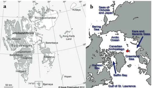
In April 2012, an 11 m long firn core was recovered from the summit of the Holtedahlfonna glacier, Spitsbergen, Svalbard (79◦09′N, 13◦23′E; 1150 m. a.s.l.) using a 4′′ aluminium
auger powered by an electric drill. The sampling location is shown in Fig. 1a. The core was drilled from the bottom of a 2.4 m snowpit, at the transition between the 2011 firn layer and the seasonal snowpack. The principal physical fea-tures of each firn core section (length, layering, dust hori-zons, ice lenses, crystallography) were recorded in the field. Stratigraphic snow samples were also collected, by inserting low density polyethylene (LDPE) vials perpendicularly into the snow-pit wall with a spatial resolution of∼5 cm down
to a depth of 2.35 m. Considering that trace element concen-trations in high altitude snow and ice samples are extremely low (ranging from ng g−1to sub-pg g−1), the samples were
collected using the same stringent anti-contamination proce-dures developed for collecting snow and firn in Antarctica (Candelone et al., 1994). All sampling tools and LDPE bot-tles were pre-cleaned with diluted ultra-pure HNO3
(Ultra-pure grade, Romil, Cambridge, UK) and then rinsed sev-eral times with ultra-pure water (UPW, Purelab Ultra Ana-lytic, Elga Lab Water, High Wycombe, UK). The scientists wore clean-room clothing and polyethylene (PE) gloves dur-ing the sampldur-ing. First, the surface of the snow-pit wall was removed with a PE scraper to avoid sampling any areas that may have been contaminated during the digging. The mass of each sample was 50 to 90 g, depending on the density of the sampled snow layer. The snowpack stratigraphy was recorded and physical parameters such as temperature, snow density, grain shape and size, and hardness indexes (hand test and Swiss Rammesonde method) were measured. The form of the snow grains and their dimensions were established ac-cording to the International Association of Cryospheric Sci-ence classification.
2.2 Sample preparation
The firn core sections were processed in a class-100 lami-nar flow hood in the laboratory of the Italian research sta-tion in Ny-Ålesund. Core secsta-tions were cut to 5 cm resolu-tion with a commercial hand saw that was carefully cleaned with methanol and UPW before each cutting operation. Pro-cessed samples were kept frozen in dark conditions to avoid any photo-activation of the halogens. The firn ice core sam-ples were decontaminated according to a simplified chis-elling procedure (Candelone et al., 1994), using a ceramic knife pre-cleaned with UPW. Three different knives were used to chisel away successive layers which may have been contaminated during drilling, handling, transport and stor-age. The decontaminated firn samples were sealed into UPW-rinsed PE bags, melted at room temperature in darkness and then aliquotted into LDPE vials. To evaluate the possibility of contamination due to sample processing, artificial ice cores produced from UPW were handled and prepared in an iden-tical manner to the samples. No external contamination was detected as a consequence of the core processing.
Snow-pit samples were transported directly to Venice, then melted at room temperature under a class 100 laminar flow bench. For halogens analysis 10 mL of melted water was transferred to 12 mL acid-cleaned LDPE vials. Other aliquots were taken for determination of stable isotope ratios and con-centrations of major and minor ions and trace elements.
2.3 Analytical methods
Concentrations of I and Br, as well as other 28 trace elements, were determined by Inductively Coupled Plasma Sector Field Mass Spectrometry (ICP-SFMS; Element2, ThermoFischer, Bremen, Germany) equipped with a cyclonic Peltier-cooled spray chamber (ESI, Omaha, US), following the methods of (Gabrielli et al., 2005). The sample flow was maintained at 0.4 mL min−1. Based on the method proposed by Bu et al. (2003), we developed an analytical procedure for the mea-surement of total Br and I in firn/ice samples. Particular at-tention was paid to maintaining a rigorous cleaning proce-dure between analyses as the measurement of these elements is sensitive to instrumental memory effects. A 24 h cleaning cycle was adopted before each analytical session to guaran-tee a stable background level. The 24 h cleaning cycle con-sisted of alternate flushing of ammonia solution 5 % (pre-pared fromTraceSELECT®ammonium hydroxide solution,
Sigma Aldrich, MO, US) for 3 min, followed by a UPW rinse lasting 30 s, and a 2 % HNO3wash (trace metal grade,
Romil, Cambridge, UK) for 3 min. Between each analysis a single NH4OH, UPW, HNO3, UPW cycle was sufficient
to ensure that the background value is achieved (difference of < 1 % compared to the initial background level). Iodine and Br were calibrated by external calibration using stan-dards of 10 to 4000 pg g−1. I and Br standards were
Fig. 1. (a)Map of the drilling site (79◦09′N, 13◦23′E; 1150 m a.s.l.) at Holtedahlfonna glacier at Spitsbergen, Svalbard (courtesy of
Nor-wegian Polar Institute).(b)Descriptive map of the Arctic sea ice regions (from NSIDC) and a red dot indicate the Spitzbergen firn core
location.
(TraceCERT® purity grade, Sigma-Aldrich, MO, USA) in UPW. All calibration curves showed correlation coefficients greater than 0.99 (df =4,p=0.05). Detection limits,
cal-culated as three times the standard deviation of the blank, were 5 and 50 pg g−1for127I and79Br, respectively.
Repro-ducibility was evaluated by repeating measurements of se-lected samples characterized by different concentration val-ues (between 20 pg g−1 and 400 pg g−1 for I and between
400 and 600 pg g−1for Br). The residual standard deviation
(RSD) was low for both halogens and ranged between 1–2 % and 2–10 % for Br and I, respectively.
A Picarro L2120-i Isotopic Liquid Water Analyzer with High Precision Vaporizer A0211 was used to measureδ18O.
The reproducibility of repeated measurements was better then±0.1 ‰. Isotopic compositions measured are reported
in the common delta units relative to standard VSMOW.
2.4 Statistical approach
We also developed a statistical segmentation of theδ18O time
series into subseries corresponding to each of the observation years from 2003 to 2011. In order to obtain this segmented series, we first applied a smoothing spline to theδ18O time
series and interpolated the series onto a regular grid. We then identified the turning points of the smoothed δ18O series,
with peaks corresponding to summer periods and troughs corresponding to winter periods. Turning-point identification was performed using Kendall information theory (Kendall, 1976) as implemented in the function “turnpoints” of the R (R Core Team, 2011) package “pastecs” (Ibanez et al., 2009). The peaks (summers) identified by this software are denoted in Fig. 2d as solid red triangles, while the troughs (winters) are denoted as solid blue inverted triangles.
Ac-cordingly, each calendar year corresponds to the period be-tween consecutive blue triangles. For the data corresponding to 2005, the algorithm automatically determined two peaks; however, when combined with Holtedahlfonna mass balance data we attributed summer to the first peak. These invalid turning points are denoted by empty red and blue triangles in Fig. 2d. The segmentation of theδ18O time series was used
to identify the %Brenrand I data pertaining to the various
ob-servation years and hence allowed the calculation of annual average values of %Brenrand I.
The significance of Pearson correlations between the an-nual averages of %Brenr and seasonal sea ice area, and
be-tween iodine fluxes and March–May sea ice extent, was eval-uated with the usual Fisher Z transform approach. P
val-ues were adjusted for multiple testing using the False Dis-covery Rate method (Benjamini and Hochberg, 1995). Here-after, correlation values,p values and adjustedp values for
testing the absence of correlation are indicated asr=xx,p
value=xx, adj.p=xx, respectively.
Pearson correlation is based on assumptions of linearity and normality that are difficult to assess with short data series. In order to avoid overinterpretation of the results, Kendall tau rank correlations were also evaluated. Kendall tau provides an alternative measure of association that it is unaffected by linearity and normality assumptions. However, given that only a short data series was available for producing the statistical comparisons in Sects. 3.2 and 3.3, we consider these findings to be preliminary and only indicative.
0.9
0.8
0.7
0.6
0.5
density (g cm
-3 )
-500 -400 -300 -200 -100 0
Depth (cm w.eq)
-18 -17 -16 -15 -14 -13
b !"
V
#
(‰ - raw data)
-17 -16 -15 -14
b
!" V
#
(‰ - smoothed)
1.00
snowpack winter/spring 2012
density density (smoothed)
thin lens medium lens
large ice layers b!"
V (‰) b!"
V (‰ - smth) summer winter
2003 2004 2005 2006 2007 2008 2009 2010 2011
mass balance (NPI)
(a)
(b)
(c)
(d)
83
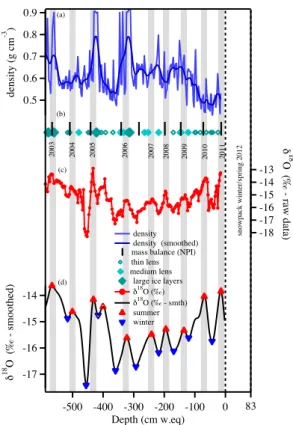
Fig. 2. 18O isotopic ratios (b) and density profiles (a) in the
Holtedahlfonna firn core. Vertical black bars(c)indicate mass
bal-ance measurements carried out at 1150 m a.s.l. in the Holtedahl-fonna glacier summit, 40 m west of the drilling site. Diamonds
(c)indicate the presence of ice lenses in the core; the increasing
size of the diamond represents increasing thickness of the lenses. These are characterized as thin (< 20 mm), medium (20–100 mm) and large (> 100 mm). These data have been used to construct the core chronology, which covers 10 yr of deposition. Statistical
as-sessment of the smoothed (smth)18O profile turnpoints(d). Solid
red triangles indicate assigned summer peaks and solid blue trian-gles indicate assigned winter troughs. Empty red and blue triantrian-gles indicate spurious assignments of summer peaks and winter troughs. The grey bars indicate summer periods as inferred from the data set.
1998) using NCEP meteorological reanalysis data (Kalnay et al., 1996) and clustered for 3 or 6 days back in time.
3 Results and discussion
3.1 Firn core chronology
Unlike the majority of the glaciers of Svalbard, the upper-most part of the Holtedahlfonna has a positive mass bal-ance and hence preserves most of its annual snow deposi-tion. Over the eight years, the net mass balance at the top of Holtedahlfonna glacier (1150 m a.s.l.) ranged from 640 to 1100 mm w.eq. (average 760±145 mm w.eq.). The
sum-mer accumulation ranged from −38 % (ablation) to +4 %
(accumulation) of the total, with an average value of−8 %
(Fig. 2b). Some melting and percolation is indicated by the presence of several ice lenses in the core (Fig. 2b); however, it has been proposed that melt events have only a minor in-fluence on the seasonal climatic signal determined from the
δ18O signal in Svalbard cores (Pohjola et al., 2002). This is
also confirmed by our results, where a clear seasonality has been detected (Fig. 2c, d) despite the presence of melt layers. The core has been dated based on the seasonal variations of
δ18O as well as from annual mass balance calculations
ob-tained from the difference between the winter accumulation and the summer melting. Mass balance estimates have been carried out through the measurement of several ablatomet-ric stakes along the Holtedahlfonna glacier. The uppermost stake is located very close to the drilling site (about 40 m) and it provides precise and accurate accumulation data of the surrounding area. For this reason, mass balance measure-ments at stake 8 are used to support isotopic dating, espe-cially when theδ18O shows ambiguities (e.g. 2005 summer
season, see Fig. 2). The shallow core and the snowpit cover the period from winter 2003 to spring 2012 (Fig. 2), with less than±1 yr uncertainty in the dating. Many factors can affect
the accurate reconstruction of local temperatures based on the Holtedahlfonnaδ18O profile, hence we only use theδ18O
profile to evaluate annual deposition cycles.
3.2 Iodine and March–May sea ice
Iodine concentrations in Holtedahlfonna glacier samples ranged from below the detection limit (5 pg g−1) to 249
pg g−1(depth 68.9 cm w.eq), with most concentrations less
than 118 pg g−1 (Fig. 3). These values were compared to
Na concentrations to ensure that marine salts did not sig-nificantly influence the I concentration at Holtedahlfonna glacier. The influence of sea salt deposition was calculated using Na as a conservative marine salt marker and consid-ering a representative value of the seawater I / Na mass ratio of 5.9×10⁻⁵(Turekian, 1968). On this basis, sea salt I was
found to consistently account for less than 2 % of iodine con-centrations.
Iodine can be emitted from the ocean in a number of ways. Firstly, via biological production and emission of a variety of organo-iodine compounds (Carpenter, 2003). Although CH3I
is the major organo-iodine species, it is photolysed relatively slowly in the atmosphere and thus is a less important source of active iodine radicals (I, IO, OIO) in the atmospheric boundary layer than photo-labile species such as CH2I2and
CH2ICl (Carpenter, 2003); secondly, by biological
produc-tion of I2from macroalgae, which is important in coastal
ar-eas (Saiz-Lopez and Plane, 2004); lastly, the uptake of O3at
the ocean surface and its reaction with iodide (I−)ions causes
the emission of HOI and I2 (Carpenter et al., 2013). It has
been postulated that algae growing under the sea ice around Antarctica produce I2 which percolates up through the ice
100
80
60
40
20 I 127
(pg g
-1
)
-400 -200 0 Depth (cm w.eq.) -18
-17 -16 -15 -14 -13
b
!" V
#$
‰
%
14.0x10⁶
13.5 13.0
average sea ice extension in km
2
(March-May)
2012 2010 2008 2006 2004
249 pg g
-1
[I]
spring sea ice extent
b!" V
# ###b!"
V spline summer top
2003 2004 2005 2006 2007 2008 2009 2010 2011
snowpack winter/spring 2012
83
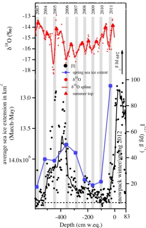
Fig. 3.Iodine concentrations in pg g−1(black circles) compared
with spring sea ice extent in km2(blue circles, reverse scale).
In-creased I concentrations in the firn core can be linked to deIn-creased
spring sea ice extension. The18O (‰) profile is shown in red. The
grey bars indicate spring-summer periods. The dotted line indicates
the iodine detection limit (5 pg g−1). Sea ice data from NSIDC.
the very high levels of IO radicals which have been observed in the coastal marine boundary layer of Antarctica (Saiz-Lopez and Boxe, 2008). In contrast, in the Arctic boundary layer the IO radical has proved to be difficult to detect, al-though recently small quantities were detected downwind of open leads or polynyas (Mahajan et al., 2010) suggesting that open ocean could be an important source of iodine instead of sea ice algae as has been proposed for Antarctica. It seems likely that the greater thickness of Arctic sea ice and its im-permeability for almost all of the period (Zhou et al., 2013) inhibits the upwelling of iodine through capillary channels in the ice (Saiz-Lopez and Boxe, 2008), and so atmospheric iodine in the Arctic is instead associated with air flow above ocean surfaces.
Considering that the main atmospheric iodine source is bi-ological primary production in colder waters, the iodide con-centration is lower (R. Chance, University of York, personal communication, 2013) and so the production of HOI and I2
from the uptake of O3at the ocean surface is less significant,
the primary biological bloom occurs around Svalbard during the March–May period (Ardyna et al., 2013), and that iodine
is primarily emitted from the open-ocean surface, we can now evaluate the change in sea ice extension around Sval-bard during the period covered by the firn core. The iodine profiles from Svalbard show two periods with high trations: between 2004–2006 and 2011–2012 where concen-trations exceeded 50 pg g−1 (Fig. 3). These higher
concen-trations can be associated with a decrease in the March–May sea ice extension (Fig. 3). In this first evaluation we use the total Arctic sea ice extension; however, a more detailed eval-uation is necessary to better understand which Arctic sectors (Fig. 1b) are most likely to influence the observed iodine de-position at Svalbard.
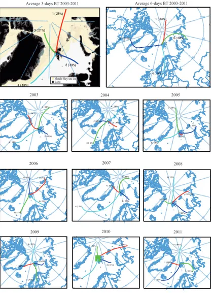
Accurate estimation of the sea ice areas influencing io-dine deposition to Svalbard is difficult due to the variabil-ity of many factors such as air mass direction and speed, exchange with the free troposphere, and deposition of io-dine compounds en route to the sampling site. The partition-ing of iodine species between aerosol gas phase is a further uncertainty (Saiz-Lopez et al., 2012). Average March–May three-day back trajectories for the period 2003–2011 from the Holtedahlfonna drilling site (Fig. 4), together with previ-ous studies (Rozwadowska et al., 2010; Eleftheriadis et al., 2009), suggest that air masses predominantly originate from the Greenland, Barents and Kara seas and the Arctic Basin. However considering the atmospheric lifetime of some or-ganic compounds (CH3I) are on the order of 2–6 days
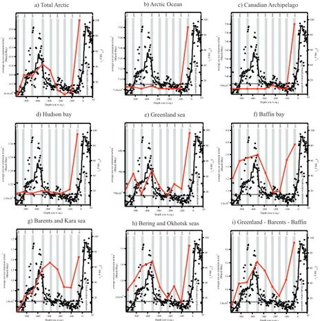
(Car-penter, 2003), we extend our back trajectory calculation to 6 days. These results confirm the influence of the above men-tioned basins but also indicate a possible influence of Baffin Bay. Back trajectory calculations suggest that the Greenland sea, Barents sea and Baffin Bay regions could be consid-ered the most important source regions for iodine. In par-ticular, excluding the Okhotsk and Bering sea, the change in March–May sea ice in these basins can explain the total Arc-tic sea ice change during the March–May period. However, if we consider the change for a single basin only a poor link with iodine is detected (Fig. 5e, f, g). Instead when we con-sider the sum of these three basins the retreat in March–May (Fig. 5i) sea ice is well mirrored by iodine concentrations in the core. These interpretations are partially confirmed by preliminary statistical results. A negative significant cor-relation is found between Iodine and Baffin (r= −0.70, p value=0.019, adj. p=0.033) and between Iodine and
Greenland sea (r= −0.63,pvalue=0.034, adj.p=0.033),
but no significant correlation is found between Iodine and Barents sea (r= −0.32,p value=0.204, adj. p=0.204).
A statistically significant negative correlation (r= −0.64,p
value=0.031, adj.p=0.038) is found when considering the
retreat in March–May sea ice of the three basins combined. However, Kendall tau rank correlation is doubtful about the presence of a significant negative association between Iodine and the three combined basins (τ = −0.5,pvalue=0.038,
adj.p=0.113). Given the discrepancy between Pearson
-30 H s t s t s
t 1 ( 14%)
Hn
o
nono 2 ( 29%)
H l m l m l m
3 ( 39%)
H s t s t s t
4 ( 18%)
2003
-90
-60
-30
0 30
60 90 120 60 s t
stst
1 ( 49%)
n o n o n o 2 ( 28%)
l m l m l m
3 ( 9%)
s t s t s t
4 ( 14%)
2004
-30
1 ( 31%)
n o n
o
n
o 2 ( 32%)
l m l m l m
3 ( 26%)
s t s t s t
4 ( 12%)
2005
-30
0 30
60 60 s t s t s t
1 ( 22%)
n o n o n o 2 ( 33%)
l m l m lm
3 ( 21%)
s
t
st
st
4 ( 24%)
2006
-90
-60
-30
0 30
60 60 s t s t s t
1 ( 39%)
n o n o n o 2 ( 32%)
l m l
mlm
3 ( 28%)
s t s t s t
4 ( 2%)
2007 60 s t s t st
1 ( 24%)
n
o
n
o
no
2 ( 26%)
l m l m l m
3 ( 34%) s
t
s
t
s
t
4 ( 16%)
2008
-60
-30
0 30
60 60 s t s t
1 ( 28%)
no
non
2 ( 24%)
l m l m l m
3 ( 13%)
s t s t s t
4 ( 35%)
2009 60 60 s t s
t s t
1 ( 14%)
no
n
ono 2 ( 41%)
l l m l m
3 ( 35%)
s t s t s t
4 ( 10%)
2010
-60
-30
0 30
60 60 s t s t s t
1 ( 39%)
n o n o n o 2 ( 22%)
lm l
m l m
3 ( 13%)
s t s t s t
4 ( 26%)
2011
-90
-60
-30
0 30
60 90 120 60 s s t s t s t s
1 ( 33%)
n o n o n o n o n o n o 2 ( 21%)
l l l l l l
3 ( 38%)
s t s t s t s t s tst
4 ( 9%)
Average 6-days BT 2003-2011 Average 3-days BT 2003-2011
H
1 ( 28%)
H
2 ( 33%)
H
3 ( 21%)
H
4 ( 18%)
March-May sea ice Land
Fig. 4.March–May back trajectory (BT) calculations using HYSPLIT during the period 2003–2011. Average 3 and 6 day back trajectories
are shown in the first top chart. Three-day back trajectory calculations for each year are also shown.
negative correlation suggests that the cover of March–May sea ice influences the iodine flux. If iodine was emitted in substantial quantities by algae blooming under the sea ice, a positive association between sea ice extension and I con-centration should have been observed. Such an interpretation is supported by differential optical absorption spectroscopy (DOAS) measurements of atmospheric iodine in the Cana-dian Arctic that show that IO concentrations become de-tectable only in the presence of open sea water (Mahajan et al., 2010). No significant IO signal was recorded when air masses flowed above solid sea ice (Mahajan et al., 2010), implying that percolation of I through the sea ice may not be a major IO emission mechanism in the Arctic.
Sturges and Barrie (1988) determined iodine and bromine concentrations in Canadian Arctic aerosol, demonstrating that I fluxes increased sharply during the March–May pe-riod. This behaviour is likely associated with the
phytoplank-ton bloom that occurs with the dawn of solar radiation in the March–May period. The variation in biological primary pro-ductivity has also been investigated in relation to the presence of open-ocean water in the Arctic (Pabi et al., 2008; Ander-son and Kaltin, 2001). However, the reaction of deposited O3
with I−at the exposed ocean surface may also make a
signif-icant contribution during summer and fall.
100 80 60 40 20 I127 (pg g -1 )
-500 -400 -300 -200 -100 0
Depth (cm w.eq.)
14.4x10⁶ 14.2 14.0 13.8 13.6 13.4 13.2 13.0
average sea ice extension in km
2 (March-May) 2012 2010 2008 2006 2004
year (sea ice)
2003 2004 2005 2006 2007 2008 2009 2010 2011
snowpack winter/spring 2012
83 a) Total Arctic
100 80 60 40 20 I127 (pg g -1 )
-500 -400 -300 -200 -100 0
Depth (cm w.eq.) 750x103
700 650
average sea ice extension in km
2 (March-May) 2012 2010 2008 2006 2004
year (sea ice)
2003 2004 2005 2006 2007 2008 2009 2010 2011
snowpack winter/spring 2012
83 e) Greenland sea
100 80 60 40 20 I127 (pg g -1 )
-500 -400 -300 -200 -100 0
Depth (cm w.eq.) 1.8x10⁶ 1.7 1.6 1.5 1.4 1.3 1.2
average sea ice extension in km
2 (March-May) 2012 2010 2008 2006 2004
year (sea ice)
2003 2004 2005 2006 2007 2008 2009 2010 2011
snowpack winter/spring 2012
83 g) Barents and Kara sea
100 80 60 40 20 I127 (pg g -1 )
-500 -400 -300 -200 -100 0
Depth (cm w.eq.) 1.4x10⁶ 1.3 1.2 1.1 1.0 0.9 0.8
average sea ice extension in km
2 (March-May) 2012 2010 2008 2006 2004
year (sea ice)
2003 2004 2005 2006 2007 2008 2009 2010 2011
snowpack winter/spring 2012
83 f) Baffin bay
100 80 60 40 20 I127 (pg g -1 )
-500 -400 -300 -200 -100 0
Depth (cm w.eq.) 3.8x10⁶
3.6 3.4 3.2 3.0
average sea ice extension in km
2 (March-May) 2012 2010 2008 2006 2004
year (sea ice)
2003 2004 2005 2006 2007 2008 2009 2010 2011
snowpack winter/spring 2012
83 i) Greenland - Barents - Baffin 100 80 60 40 20 I127 (pg g -1 )
-500 -400 -300 -200 -100 0
Depth (cm w.eq.)
1.24x10⁶
1.22 1.20 1.18 1.16
average sea ice extension in km
2 (March-May) 2012 2010 2008 2006 2004
year (sea ice)
2003 2004 2005 2006 2007 2008 2009 2010 2011
snowpack winter/spring 2012
83 d) Hudson bay
100 80 60 40 20 I127 (pg g -1 )
-500 -400 -300 -200 -100 0
Depth (cm w.eq.)
7.16x10⁶ 7.14 7.12 7.10 7.08 7.06 7.04
average sea ice extension in km
2 (March-May) 2012 2010 2008 2006 2004
year (sea ice)
2003 2004 2005 2006 2007 2008 2009 2010 2011
snowpack winter/spring 2012
83 b) Arctic Ocean
100 80 60 40 20 I127 (pg g -1 )
-500 -400 -300 -200 -100 0
Depth (cm w.eq.)
750x103 748 746 744 742 740 738 736
average sea ice extension in km
2 (March-May) 2012 2010 2008 2006 2004
year (sea ice)
2003 2004 2005 2006 2007 2008 2009 2010 2011
snowpack winter/spring 2012
83 c) Canadian Archipelago
100 80 60 40 20 I127 (pg g -1 )
-500 -400 -300 -200 -100 0
Depth (cm w.eq.) 2.0x10⁶
1.8 1.6 1.4
average sea ice extension in km
2 (March-May) 2012 2010 2008 2006 2004
year (sea ice)
2003 2004 2005 2006 2007 2008 2009 2010 2011
snowpack winter/spring 2012
83 h) Bering and Okhotsk seas
Fig. 5.Comparison of Iodine trend in the firn core recovered with changes in March–May sea ice from single sectors. Panel(g)shows the
sum of the Greenland sea, Barents sea and Baffin bay regions.
signal as well as those of other less-reactive species (Pohjola et al., 2002). In such a case, Iodine concentrations will not show an annual cycle but could still be indicative of mean annual Iodine deposition. Though our data suggest a link-age between March–May sea ice retreat and iodine emission we need to consider the relationship between these two pa-rameters. The iodine signal suggests that changes in the Bar-ents, Kara and Greenland seas and Baffin Bay are likely to be the main sources for Iodine deposited in Svalbard. How-ever we need to consider that the observed 30–50 % change of March–May sea ice in these regions results in a tenfold change in the iodine signal. In the Arctic it appears likely that non-linear processes are involved in the emission, transport and/or deposition of iodine. This may be due to non-linear biological responses to ocean water coverage, or the addi-tional influence of other factors such as nutrient availability. An alternative could be that the iodine observed at Svalbard actually originates from quite small and specific regions of open water that are being expanded by a much larger fac-tor, but whose area is related to the general retreat of the ice. It is not possible to speculate further on such non-linear re-sponses to sea ice change until Iodine emission sources are better known.
3.3 Bromine enrichment and seasonal sea ice
Bromine concentrations in Holtedahlfonna glacier samples ranged from 0.43 to 7.36 ng g−1. As with Na, sea water is the
primary emission source of atmospheric Br. Although the to-tal Br concentration has a statistically significant positive as-sociation with Na (r=0.78,pvalue < 0.001), Br could have
an additional atmospheric production source which must be accounted for. Br2 is produced by the uptake of HOBr on
brine and snow covered (including frost flowers) first year sea ice. Photolysis of Br2then produces Br atoms which
re-act with HO2 radicals to reform HOBr, thus setting up an
efficient auto-catalytic cycle known as a bromine explosion (Pratt et al., 2013). Once in the gas phase, the major sink for bromine is HBr, formed by the reaction of Br atoms with HCHO. HBr can then be deposited as bromide ions in the snowpack. In order to evaluate the sensitivity of Br as a tracer of sea ice extension, it is necessary to remove the sea spray component by applying a correction based on the Br / Na mass ratio in sea water. We used a Br / Na mass ratio value of 0.006 (Millero, 1974). The bromine enrich-ment percentage (%Brenr)was calculated using the formula
(([Brice]/([Naice]×0.006)×100)−100), where a value of
600
500
400
300
200
100
0
% Br
enr
-500 -250 0
Depth cm w. eq
11.0x10⁶
10.5
10.0
9.5
9.0
8.5
seasonal sea ice (km
2
)
2012 2010 2008 2006 2004
-18 -17 -16 -15 -14 -13
b
!" V
#$
‰)
2011
2010
2009
2008
2007
2006
2005
2004
2003
Average extension of seasonal sea ice
Brenr
Brenr spline
b!" O (‰)
b!" O spline summer top
83
snowpack winter/spring 2012
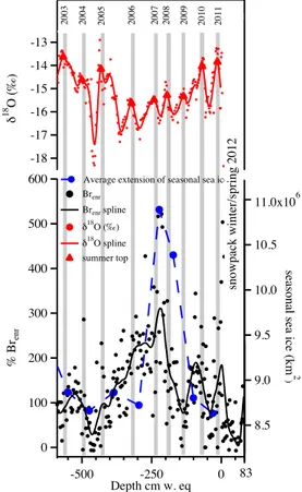
Fig. 6.Bromine enrichment (%Brenr, black circles) is compared to seasonal sea ice area (blue circles). Seasonal sea ice area was cal-culated as the difference between the March maxima of sea ice and the September sea ice minima of the previous year. Seasonal
vari-ability of %Brenris present in the upper part of the core. Bromine
is enriched relative to seawater Na during the springtime, when the seasonal sea ice-produced Bromine explosion is most active. The grey bars indicate summer periods. Sea ice data from NSIDC.
compared to the Br / Na mass ratio. Hence, only positive %Brenr values indicate production of Br as a result of the
Br explosion.
The Holtedahlfonna glacier firn core record indicates that Br is almost always enriched beyond representative seawater values, in some cases up to 6 times in 2008 (Fig. 6). Only a few samples are slightly depleted below seawater values. We find rather constant %Brenrvalues of approximately 100
between 2003 and 2005, followed by a steady increase to a maximum of 350 in 2008 and then a return to values of approximately 100 between 2009 and 2012.
Sturges and Barrie (1988) and Toom-Sauntry et al. (2002) reported higher concentrations of Br in aerosol from March to May with a maximum in April. The consistent spring-time enrichment of Br, beyond concentrations expected from solely marine salt inputs, suggests that the springtime peak of bromine explosion activity is the main source for addi-tional Br deposited in Svalbard glaciers. Bromine is a
partic-ularly active element above seasonal sea ice during spring-time. Satellite and field-based observations clearly show the springtime increase of atmospheric BrO concentrated above first-year sea ice (Nghiem et al., 2012; Pratt et al., 2013). The highest Arctic atmospheric BrO values are located above the seasonal sea ice and decrease above the older multiyear sea ice toward the seasonal sea ice margin (Richter et al., 1998; Sihler et al., 2012; Theys et al., 2011).
With these findings we compare %Brenrwith Arctic
sea-sonal sea ice extension, where seasea-sonal sea ice was calcu-lated by subtracting the September (minimum) sea ice area from the March (maximum) sea ice area of the following year (Cavalieri et al., 1996). As was the case for I, we ini-tially evaluate the %Brenrversus the total Arctic seasonal sea
ice extent (Fig. 7a). The results obtained from the Holtedahl-fonna glacier firn core show a positive relationship between seasonal sea ice area and %Brenr. Both parameters increased
after 2005 to a maximum in 2008, followed by lower val-ues from 2009 to 2012. The similar trends of %Brenrto those
of seasonal sea ice area seem to support our interpretation that absolute %Brenr values are consistent with a sea
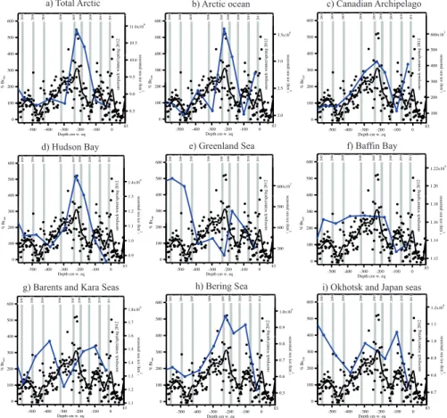
ice-related source of Br production. Using the total Arctic sea ice extension may not be appropriate, so we have evaluated the change in seasonal sea ice for the various Arctic sec-tors (Fig. 7) and the path of 3 day back trajectories for in-dividual years and on average during the period 2003–2011 (Fig. 5). Considering the relatively fast deposition velocity of gas phase bromine (HBr), it is likely that the enrichment of bromine is more regionally influenced than for iodine. Back trajectories suggest that two possible sources are the Arctic Ocean and the Canadian Archipelago (Fig. 4). The south-ward back trajectories seem not to cross sea ice regions how-ever we cannot exclude the influence of the ice-covered ar-eas of the Greenland and Barents sar-eas. In contrast, the in-fluence of the Bering and Okhotsk seas can be considered negligible. We plotted the changes in seasonal sea ice for each region (Fig. 7) with the bromine enrichment and find a good agreement when we consider the changing seasonal sea ice in the Arctic Ocean (Fig. 7b), Canadian Arctic (Fig. 7c) and Hudson Bay (Fig. 7d). While the influence of the Arctic Ocean and Canadian Archipelago seem to also be confirmed by back trajectory calculations, the influence of Hudson Bay Br sources seems unlikely. The poor agreement between the %Brenrand seasonal sea ice in the Greenland and Barents seas
suggest a negligible role also for these sea ice regions. In parallel with these qualitative interpretations we also calculated statistical correlations. As for iodine, due to the short data series, we need to consider these results indica-tive and preliminary. However, the statistical analysis sug-gests a positive correlation with Arctic Ocean (r=0.81,p
value=0.008, adj. p=0.036) and Canadian Archipelago
(r=0.92,pvalue=0.001, adj.p=0.006). Kendall tau
sug-gests a somehow weaker significance for both Arctic Ocean (tau=0.71,pvalue=0.007, adj.p=0.064) and Canadian
600 500 400 300 200 100 0 % Br enr
-500 -400 -300 -200 -100 0 Depth cm w. eq
3.5x10⁶
3.0
2.5
2.0
seasonal sea ice (km
2 ) 2012 2010 2008 2006 2004 2011 2010 2009 2008 2007 2006 2005 2004 2003 83
snowpack winter/spring 2012
b) Arctic ocean
600 500 400 300 200 100 0 % Br enr
-500 -400 -300 -200 -100 0 Depth cm w. eq
11.0x10⁶ 10.5 10.0 9.5 9.0 8.5
seasonal sea i
ce (km 2 ) 2012 2010 2008 2006 2004 2011 2010 2009 2008 2007 2006 2005 2004 2003 83
snowpack winter/spring 2012
a) Total Arctic
600 500 400 300 200 100 0 % Br enr
-500 -400 -300 -200 -100 0 Depth cm w. eq
600x103 500 400 300 200 100
seasonal sea ice (km
2 ) 2012 2010 2008 2006 2004 2011 2010 2009 2008 2007 2006 2005 2004 2003 83
snowpack winter/spring 2012
c) Canadian Archipelago
600 500 400 300 200 100 0 % Br enr
-500 -400 -300 -200 -100 0 Depth cm w. eq
1.8x10⁶ 1.7 1.6 1.5 1.4 1.3 1.2 1.1 seaso n al s
ea ice (k
m 2 ) 2012 2010 2008 2006 2004 2011 2010 2009 2008 2007 2006 2005 2004 2003 83
snowpack winter/spring 2012
g) Barents and Kara Seas
600 500 400 300 200 100 0 % Br enr
-500 -400 -300 -200 -100 0 Depth cm w. eq
600x103
500
400
300
seasonal sea ice (km
2 ) 2012 2010 2008 2006 2004 2011 2010 2009 2008 2007 2006 2005 2004 2003 83
snowpack winter/spring 2012
e) Greenland Sea
600 500 400 300 200 100 0 % Br enr
-500 -400 -300 -200 -100 0 Depth cm w. eq
1.22x10⁶ 1.20 1.18 1.16 1.14 1.12
seasonal sea ice (km
2 ) 2012 2010 2008 2006 2004 2011 2010 2009 2008 2007 2006 2005 2004 2003 83
snowpack winter/spring 2012
f) Baffin Bay
600 500 400 300 200 100 0 % Br enr
-500 -400 -300 -200 -100 0 Depth cm w. eq
1.4x10⁶ 1.3 1.2 1.1 1.0 0.9
seasonal sea ice (km
2 ) 2012 2010 2008 2006 2004 2011 2010 2009 2008 2007 2006 2005 2004 2003 83
snowpack winter/spring 2012
d) Hudson Bay
600 500 400 300 200 100 0 % Br enr
-500 -400 -300 -200 -100 0 Depth cm w. eq
1.0x10⁶ 0.9 0.8 0.7 0.6 0.5
seasonal sea ice (km
2 ) 2012 2010 2008 2006 2004 2011 2010 2009 2008 2007 2006 2005 2004 2003 83
snowpack winter/spring 2012
h) Bering Sea
600 500 400 300 200 100 0 % Br enr
-500 -400 -300 -200 -100 0 Depth cm w. eq
1.2x10⁶ 1.1 1.0 0.9 0.8 0.7
seasonal sea ice (km
2 ) 2012 2010 2008 2006 2004 2011 2010 2009 2008 2007 2006 2005 2004 2003 83
snowpack winter/spring 2012
i) Okhotsk and Japan seas
Fig. 7.Comparison of %Brenrtrend in the firn core recovered with changes in seasonal sea ice from single Arctic sectors.
The change in Arctic Ocean seasonal sea ice is in good agree-ment with the change in %Brenrwith both showing maxima
between 2008 and 2009. However in 2007 there is some dis-agreement with a decrease in Arctic Ocean seasonal sea ice and an increase of %Brenr. The March–May back trajectories
of 2007 show an enhanced influence of the sea ice region at the north of Greenland. It is therefore possible that during 2007 an increase in the influence of Canadian Archipelago sea ice could have had more effect on %Brenr.
Though we suggest that the main driver of bromine en-richment found in the shallow firn core are chemical reac-tions connected to seasonal sea ice, the role of biological Br emissions was also evaluated. If biological emissions were to play an important role then a positive correlation would be expected between I and %Brenr. In the data presented here,
these two parameters show a statistically significant negative association of−0.32 (p value < 0.001) suggesting that their
fluxes are controlled by opposing sources and/or processes. We suggest that a decrease in seasonal sea ice area causes a decrease in the area available to support the Br explosion. Simultaneously, decreased seasonal sea ice contributes to a reduced March–May sea ice extent and hence increased I emission from the open water surface of the Arctic region.
We consider also the post-depositional processes affecting the Br concentration in the surface snowpack. For instance, the uptake of species such as HOBr and HOI in the snowpack could recycle bromide ions to the gas phase as Br2and IBr,
respectively.
Pratt et al. (2013) suggest that two parameters, pH and the Br−/ Cl molar ratio, could be used to identify potential
bromine emission. Though we do not measure Cl, this can be calculated from sodium concentrations using their abun-dances in sea water (Krnavek et al., 2012; Bigler et al., 2006). The first 5 cm present a pH of 4.9 and a Br−/ Cl ratio of
1/57 suggesting the possibility of bromine re-emission. All
the other samples present greater pH values, with an aver-age of 5.3 and an averaver-age Br−/ Cl ratio of 1/333. It is
pos-sible that some re-emission of bromine could occur on the fresh snow surface, as suggested by Pratt et al. (2013), how-ever the snow just below 5 cm does not present favourable conditions for gas-phase bromine release. If recycling pro-cesses were significant, then %Brenrwould be negative,
rep-resenting an overall depletion of Br relative to the marine sea salt value. Percolation, as discussed for iodine, is another process that could disturb the signal. Detecting the seasonal variation in the18O signal is not a guarantee that all other
et al. (2002).δ18O exhibits less susceptibility to changes
in-duced by melt-water percolation, compared to soluble and/or volatile acid species. Ionic compounds suffer partly from melt-water percolation but are still able to preserve their at-mospheric signal with annual resolution. The loss of season-ality below 150 cm w.eq. in our %Brenrcould be explained by
the smoothing effect of percolation due to the warmer period between 2007 and 2009 with an enhance of the number of summer positive air temperature (Bednorz and Kolendowicz, 2013). In upper part of the firn core we clearly distinguish the seasonality suggesting that bromine explosion events are recorded in the snow deposition as detected by satellite and aerosol measurement. As for iodine it appears more likely that seasonality has been affected, but the annual signal is preserved. The maximum in seasonal sea ice extension dur-ing the firn core has been reached in 2008 where we detect the maximum bromine enrichment. We cannot exclude that the %Brenrsignal was modified but the data are consistent
with observed changes in seasonal sea ice extension. As for iodine we cannot deduce from the data the relationship be-tween change in seasonal sea ice and %Brenr. Our results
suggest that for a 10 % change in overall sea ice we have a doubling of bromine enrichment. One possibility is that the Br reaching Svalbard originates from a more specific region whose sea ice area is being changed by a much larger factor. However, we must consider that also the atmospheric trans-port and the irregular occurrence of bromine explosion events complicate the identification of predictive relationships.
4 Future development
Iodine and Br profiles determined in a Holtedahlfonna glacier firn core demonstrate variability that can be related to changes in March–May sea ice extent and seasonal sea ice area during the past decade. The enrichment of Br in ice, relative to the sea salt proxy Na, can be attributed to the bromine explosion that occurs above seasonal sea ice during early spring, especially in the regions of the Arctic Ocean and Canadian Archipelago suggesting that the annual variation of %Brenrcould be mainly influenced by the variation in the
seasonal sea ice extension. Results suggest that the predom-inant Br enrichment occurs during spring and early summer; however, the likely percolation effect could have disturbed and smoothed the original signal. While Br is influenced by the variation of seasonal sea ice area, iodine in Arctic region seems primarily emitted from open water and thus related to the changes in the March–May sea ice extent. In particular, the retreat of March–May sea ice appears to be related to increased I concentrations, resulting from the increased bio-logical productivity associated with open water and the re-action of O3with iodide ions in the sea surface layer. On the
basis of this limited data set, only tentative findings can be re-ported here. Further studies will be necessary to thoroughly understand and characterize the processes controlling I and
Br transport and deposition in snow pack. The effect of per-colation and possible re-emission after deposition should be investigated, considering the presence of summer melt layers such as those observed in the Holtedahlfonna glacier and the atmospheric reactivity of these two halogens. The data pre-sented here provide a provisional basis for linking I and Br to sea ice variability, which could lead eventually to recon-struction of past sea ice variations in the polar regions.
Acknowledgements. This work was supported by the Italian
National Research Council (CNR), the Italian Ministry of Research through the PRIN project 2009 and by the EU Regional Develop-ment Foundation, project 3.2.0801.12-0044. The authors are rateful to R. Sparapani and E. Liberatori (CNR) for logistical assistance, H. Sevestre and UNIS (The University Centre in Svalbard) for supporting the field operations, and L. Poto (University of Venice) for helpful discussions regarding marine biology.
Edited by: E. Wolff
References
Aagaard, K. and Carmack, E. C.: The Role of Sea Ice and Other Fresh Water in the Arctic Circulation, J. Geophys. Res., 94, 14485–14498, 1989.
Anderson, L. G. and Kaltin, S.: Carbon fluxes in the Arctic Ocean – potential impact by climate change, Polar Res., 20, 225–232, 2001.
Ardyna, M., Babin, M., Gosselin, M., Devred, E., Bélanger, S., Matsuoka, A., and Tremblay, J.-É.: Parameterization of verti-cal chlorophyll a in the Arctic Ocean: impact of the subsur-face chlorophyll maximum on regional, seasonal, and annual primary production estimates, Biogeosciences, 10, 4383–4404, doi:10.5194/bg-10-4383-2013, 2013.
Atkinson, H. M., Huang, R.-J., Chance, R., Roscoe, H. K., Hughes, C., Davison, B., Schönhardt, A., Mahajan, A. S., Saiz-Lopez, A., Hoffmann, T., and Liss, P. S.: Iodine emissions from the sea ice of the Weddell Sea, Atmos. Chem. Phys., 12, 11229–11244, doi:10.5194/acp-12-11229-2012, 2012.
Bednorz, E. and Kolendowicz, L.: Summer mean daily air temper-ature extremes in Central Spitsbergen, Theor. Appl. Climatol., 113, 471–479, doi:10.1007/s00704-012-0798-4, 2013.
Benjamini, Y. and Hochberg, Y.: Controlling the False Discov-ery Rate: A Practical and Powerful Approach to Multiple Test-ing, J. R. Stat. Soc., Series B (Methodological), 57, 289–300, doi:10.2307/2346101, 1995.
Bigler, M., Röthlisberger, R., Lambert, F., Stocker, T. F., and Wa-genbach, D.: Aerosol deposited in East Antarctica over the last glacial cycle: Detailed apportionment of continental and sea-salt contributions, J. Geophys. Res.-Atmos., 111, D08205, doi:10.1029/2005jd006469, 2006.
Candelone, J.-P., Hong, S., and Boutron, C.: An improved method for decontaminating polar snow or ice cores for heavy metal anal-ysis, Anal. Chim. Acta., 299, 9–16, 1994.
Carpenter, L. J.: Iodine in the Marine Boundary Layer, Chemical Reviews, 103, 4953–4962, 2003.
Carpenter, L. J., MacDonald, S. M., Shaw, M. D., Kumar, R., Saun-ders, R. W., Parthipan, R., Wilson, J., and Plane, J. M. C.: At-mospheric iodine levels influenced by sea surface emissions of inorganic iodine, Nature Geosci., 6, 108–111, 2013.
Cavalieri, D. J., Parkinson, C. L., Gloersen, P., and Zwally, A. H.: Sea Ice Concentrations from Nimbus-7 SMMR and DMSP SSM/I-SSMIS Passive Microwave Data, Boulder, Col-orado USA: NASA DAAC at the National Snow and Ice Data Center., 1996.
Cronin, T. M., Smith, S. A., Eynaud, F., O’Regan, M., and King, J.: Quaternary paleoceanography of the central Arctic based on Integrated Ocean Drilling Program Arctic Coring Expedition 302 foraminiferal assemblages, Paleoceanography, 23, PA1S18, 2008.
Curran, M. A. J., van Ommen, T. D., Morgan, V. I., Phillips, K. L., and Palmer, A. S.: Ice Core Evidence for Antarctic Sea Ice Decline Since the 1950s, Science, 302, 1203–1206, 2003. Darby, D. A.: Sources of sediment found in sea ice from the
western Arctic Ocean, new insights into processes of en-trainment and drift patterns, J. Geophys. Res., 108, 3257, doi:10.1029/2002JC001350, 2003.
Draxler R. R. and Hess, G. D.: An overview of the HYSPLIT 4 modelling system for trajectories, dispersion and deposition, Aust. Meteorol. Mag., 47, 295–308, 1998.
Durner, G. M., Douglas, D. C., Nielson, R. M., Amstrup, S. C., Mc-Donald, T. L., Stirling, I., Mauritzen, M., Born, E. W., Wiig, O., DeWeaver, E., Serreze, M. C., Belikov, S. E., Holland, M. M., Maslanik, J., Aars, J., Bailey, D. A., and Derocher, A. E.: Pre-dicting 21st-century polar bear habitat distribution from global climate models, Ecol. Monogr., 79, 25–58, 2009.
Eleftheriadis, K., Vratolis, S., and Nyeki, S.: Aerosol black car-bon in the European Arctic: Measurements at Zeppelin station, Ny-Alesund, Svalbard from 1998–2007, Geophys. Res. Lett., 36, L02809, doi:10.1029/2008GL035741, 2009.
Fahl, K. and Stein, R.: Modern seasonal variability and deglacial/Holocene change of central Arctic Ocean sea-ice cover: New insights from biomarker proxy records, Earth Planet. Sc. Lett., 351, 123–133, 2012.
Fan, S.-M. and Jacob, D. J.: Surface ozone depletion in Arctic spring sustained by bromine reactions on aerosols, Nature, 359, 522–524, 1992.
Francis, J. A., Chan, W., Leathers, D. J., Miller, J. R., and Veron, D. E.: Winter Northern Hemisphere weather patterns remember summer Arctic sea-ice extent, Geophys. Res. Lett., 36, L07503, doi:10.1029/2009GL037274, 2009.
Gabrielli, P., Planchon, F. A. M., Hong, S., Lee, K. H., Hur, S. D., Barbante, C., Ferrari, C. P., Petit, J. R., Lipenkov, V. Y., Cescon, P., and Boutron, C. F.: Trace elements in Vostok Antarctic ice during the last four climatic cycles, Earth Planet. Sc. Lett., 234, 249–259, 2005.
Holland, M. M., Bitz, C. M., Eby, M., and Weaver, A. J.: The Role of Ice-Ocean Interactions in the Variability of the North Atlantic Thermohaline Circulation, J. Climate, 14, 656–675, 2001.
Ibanez, F., Grosjean, P., and Etienne, M.: Pastecs: Package for Anal-ysis of Space-Time Ecological Series, R package version, 1, 3– 11, 2009.
Isaksson, E., Kekonen, T., Moore, J., and Mulvaney, R.: The methanesulfonic acid (MSA) record in a Svalbard ice core, Ann. Glaciol., 42, 345–351, 2005.
Kaleschke, L., Richter, A., Burrows, J., Afe, O., Heygster, G., Notholt, J., Rankin, A., Roscoe, H., Hollwedel, J., and Wagner, T.: Frost flowers on sea ice as a source of sea salt and their in-fluence on tropospheric halogen chemistry, Geophys. Res. Lett., 31, L16114, doi:10.1029/2004GL020655, 2004.
Kalnay, E., Kanamitsu, M., Kistler, R., Collins, W., Deaven, D., Gandin, L., Iredell, M., Saha, S., White, G., Woollen, J., Zhu, Y., Leetmaa, A., Reynolds, R., Chelliah, M., Ebisuzaki, W., Hig-gins, W., Janowiak, J., Mo, K. C., Ropelewski, C., Wang, J., Jenne, R., and Joseph, D.: The NCEP/NCAR 40-Year Reanalysis Project, B. Am. Meteorol. Soc., 77, 437–471, doi:10.1175/1520-0477(1996)077<0437:tnyrp>2.0.co;2, 1996.
Kendall, M. G.: Time-serie, 2nd ed., Charles Griffin & Co, London, 1976.
Kinnard, C., Zdanowicz, C. M., Fisher, D. A., Isaksson, E., de Ver-nal, A., and Thompson, L. G.: Reconstructed changes in Arctic sea ice over the past 1,450 years, Nature, 479, 509–512, 2011. Krnavek, L., Simpson, W. R., Carlson, D., Domine, F.,
Dou-glas, T. A., and Sturm, M.: The chemical composition of surface snow in the Arctic: Examining marine, terrestrial, and atmospheric influences, Atmos. Environ., 50, 349–359, doi:10.1016/j.atmosenv.2011.11.033, 2012.
Lisitzin, A. P.: Sea-ice and Iceberg Sedimentation in the Ocean: Recent and Past, edited by: Springer-Verlag, Berlin, Heidelberg, 2002.
Mahajan, A. S., Shaw, M., Oetjen, H., Hornsby, K. E., Carpen-ter, L. J., Kaleschke, L., Tian-Kunze, X., Lee, J. D., Moller, S. J., Edwards, P., Commane, R., Ingham, T., Heard, D. E., and Plane, J. M. C.: Evidence of reactive iodine chemistry in the Arctic boundary layer, J. Geophys. Res., 115, D20303, doi:10.1029/2009JD013665, 2010.
Millero, F. J.: The Physical Chemistry of
Seawa-ter, Annu. Rev. Earth Planet. Sci., 2, 101–150,
doi:10.1146/annurev.ea.02.050174.000533, 1974.
Nghiem, S. V., Rigor, I. G., Richter, A., Burrows, J. P., Shepson, P. B., Bottenheim, J., Barber, D. G., Steffen, A., Latonas, J., Wang, F., Stern, G., Clemente-Colòn, P., Martin, S., Hall, D. K., Kaleschke, L., Tackett, P., Neumann, G., and Asplin, M. G.: Field and satellite observations of the formation and distribution of Arctic atmospheric bromine above a rejuvenated sea ice cover, J. Geophys. Res., 117, D00S05, doi:10.1029/2011JD016268, 2012. O’Dwyer, J., Isaksson, E., Vinje, T., Jauhiainen, T., Moore, J., Po-hjola, V., Vaikmäe, R., and van de Wal, R. S. W.: Methanesul-fonic acid in a Svalbard Ice Core as an indicator of ocean climate, Geophys. Res. Lett., 27, 1159–1162, 2000.
Pabi, S., van Dijken, G. L., and Arrigo, K. R.: Primary production in the Arctic Ocean, 1998–2006, J. Geophys. Res., 113, C08005, doi:10.1029/2007JC004578, 2008.
Petit, J. R., Jouzel, J., Raynaud, D., Barkov, N. I., Barnola, J. M., Basile, I., Bender, M., Chappellaz, J., Davis, M., Delaygue, G., Delmotte, M., Kotlyakov, V. M., Legrand, M., Lipenkov, V. Y., Lorius, C., Pepin, L., Ritz, C., Saltzman, E., and Stievenard, M.: Climate and atmospheric history of the past 420,000 years from the Vostok ice core, Antarctica, Nature, 399, 429–436, 1999. Pohjola, V. A., Moore, J. C., Isaksson, E., Jauhiainen, T., van de
Wal, R. S. W., Martma, T., Meijer, H. A. J., and Vaikmäe, R.: Effect of periodic melting on geochemical and isotopic signals in an ice core from Lomonosovfonna, Svalbard, J. Geophys. Res.-Atmos., 107, 1–14, 2002.
Polyak, L., Alley, R. B., Andrews, J. T., Brigham-Grette, J., Cronin, T. M., Darby, D. A., Dyke, A. S., Fitzpatrick, J. J., Funder, S., Holland, M., Jennings, A. E., Miller, G. H., O’Regan, M., Savelle, J., Serreze, M., St. John, K., White, J. W. C., and Wolff, E.: History of sea ice in the Arctic, Quaternary Sci. Rev., 29, 1757–1778, 2010.
Pratt, K. A., Custard, K. D., Shepson, P. B., Douglas, T. A., Pohler, D., General, S., Zielcke, J., Simpson, W. R., Platt, U., Tanner, D. J., Gregory Huey, L., Carlsen, M., and Stirm, B. H.: Pho-tochemical production of molecular bromine in Arctic surface snowpacks, Nature Geosci., 6, 351–356, doi:10.1038/ngeo1779, 2013.
R Core Team: R – A language and environment for statistical com-puting, R Foundation for Statistical, Vienna, 2011.
Rampal, P., Weiss, J., Dubois, C., and Campin, J. M.: IPCC cli-mate models do not capture Arctic sea ice drift acceleration: Consequences in terms of projected sea ice thinning and decline, J. Geophys. Res., 116, C00D07, doi:10.1029/2011JC007110, 2011.
Rankin, A. M., Auld, V., and Wolff, E. W.: Frost flowers as a source of fractionated sea salt aerosol in the polar regions, Geophys. Res. Lett., 27, 3469–3472, 2000.
Richter, A., Wittrock, F., Eisinger, M., and Burrows, J. P.: GOME observations of tropospheric BrO in northern hemispheric spring and summer 1997, Geophys. Res. Lett., 25, 2683–2686, 1998. Roscoe, H. K., Brooks, B., Jackson, A. V., Smith, M. H.,
Walker, S. J., Obbard, R. W., and Wolff, E. W.: Frost flow-ers in the laboratory: Growth, characteristics, aerosol, and the underlying sea ice, J. Geophys. Res.-Atmos., 116, D12301, doi:10.1029/2010jd015144, 2011.
Rozwadowska, A., Zielin’ski, T., Petelski, T., and Sobolewski, P.: Cluster analysis of the impact of air back-trajectories on aerosol optical properties at Hornsund, Spitsbergen, Atmos. Chem. Phys., 10, 877–893, doi:10.5194/acp-10-877-2010, 2010. Saiz-Lopez, A. and Boxe, C. S.: A mechanism for biologically-induced iodine emissions from sea-ice, Atmos. Chem. Phys. Dis-cuss., 8, 2953–2976, doi:10.5194/acpd-8-2953-2008, 2008. Saiz-Lopez, A. and Plane, J.: Novel iodine chemistry in the
marine boundary layer, Geophys. Res. Lett., 31, L04112, doi:10.1029/2003GL019215, 2004.
Saiz-Lopez, A., Chance, K., Liu, X., Kurosu, T. P., and Sander, S. P.: First observations of iodine oxide from space, Geophys. Res. Lett., 34, L12812, doi:10.1029/2007GL030111, 2007.
Saiz-Lopez, A., Plane, J. M. C., Baker, A. R., Carpenter, L. J., von Glasow, R., Gomez Martin, J. C., McFiggans, G., and Saun-ders, R. W.: Atmospheric Chemistry of Iodine, Chem. Rev., 112, 1773–1804, 2012.
Schönhardt, A., Richter, A., Wittrock, F., Kirk, H., Oetjen, H., Roscoe, H. K., and Burrows, J. P.: Observations of iodine monox-ide columns from satellite, Atmos. Chem. Phys., 8, 637–653, doi:10.5194/acp-8-637-2008, 2008.
Schönhardt, A., Begoin, M., Richter, A., Wittrock, F., Kaleschke, L., Gómez Martín, J. C., and Burrows, J. P.: Simultaneous satel-lite observations of IO and BrO over Antarctica, Atmos. Chem. Phys., 12, 6565–6580, doi:10.5194/acp-12-6565-2012, 2012. Serreze, M. C., Maslanik, J. A., Scambos, T. A., Fetterer, F.,
Stroeve, J., Knowles, K., Fowler, C., Drobot, S., Barry, R. G., and Haran, T. M.: A record minimum arctic sea ice extent and area in 2002, Geophys. Res. Lett., 30, 1110, doi:10.1029/2002gl016406, 2003.
Sihler, H., Platt, U., Beirle, S., Marbach, T., Kühl, S., Dörner, S., Verschaeve, J., Frieß, U., Pöhler, D., Vogel, L., Sander, R., and Wagner, T.: Tropospheric BrO column densities in the Arctic derived from satellite: retrieval and comparison to ground-based measurements, Atmos. Meas. Tech., 5, 2779– 2807, doi:10.5194/amt-5-2779-2012, 2012.
Simpson, W. R., Carlson, D., Hönninger, G., Douglas, T. A., Sturm, M., Perovich, D., and Platt, U.: First-year sea-ice contact predicts bromine monoxide (BrO) levels at Barrow, Alaska better than potential frost flower contact, Atmos. Chem. Phys., 7, 621–627, doi:10.5194/acp-7-621-2007, 2007.
Smith, B. T., Van Ommen, T. D., and Curran, M. A. J.: Methane-sulphonic acid movement in solid ice cores, Ann. Glaciol., 39, 540–544, doi:10.3189/172756404781814645, 2004.
Stern, H. L., Rothrock, D. A., and Kwok, R.: Open water production in Arctic sea ice: Satellite measurements and model parameteri-zations, J. Geophys. Res., 100, 20601–20612, 1995.
Stroeve, J., Holland, M. M., Meier, W., Scambos, T., and Serreze, M.: Arctic sea ice decline: Faster than forecast, Geophys. Res. Lett., 34, L09501, doi:10.1029/2007GL029703, 2007.
Sturges, W. T. and Barrie, L. A.: Chlorine, Bromine and Iodine in arctic aerosols, Atmos. Environ., 22, 1179–1194, 1988. Theys, N., Van Roozendael, M., Hendrick, F., Yang, X., De Smedt,
I., Richter, A., Begoin, M., Errera, Q., Johnston, P. V., Kreher, K., and De Mazière, M.: Global observations of tropospheric BrO columns using GOME-2 satellite data, Atmos. Chem. Phys., 11, 1791–1811, doi:10.5194/acp-11-1791-2011, 2011.
Toom-Sauntry, D. and Barrie, L. A.: Chemical composition of snowfall in the high Arctic: 1990–1994, Atmos. Environ., 36, 2683–2693, doi:10.1016/S1352-2310(02)00115-2, 2002. Turekian, K. K.: Oceans, Prentice-Hall, 1968.
Vare, L. L., Massé, G., Gregory, T. R., Smart, C. W., and Belt, S. T.: Sea ice variations in the central Canadian Arctic Archipelago during the Holocene, Quaternary Sci. Rev., 28, 1354–1366, 2009. Wang, M. and Overland, J. E.: A sea ice free summer Arctic within 30 years: An update from CMIP5 models, Geophys. Res. Lett., 39, L18501, doi:10.1029/2012GL052868, 2012.
Warren, B. A.: Why is no deep water formed in the North Pacific?, J. Mar. Res., 41, 327–347, 1983.
Gas-pari, V.: Southern Ocean sea-ice extent, productivity and iron flux over the past eight glacial cycles, Nature, 440, 491–496, 2006. Wolff, E., Barbante, C., Becagli, S., Bigler, M., Boutron, C.,
Castel-lano, E., De Angelis, M., Federer, U., Fischer, H., and Fundel, F.: Changes in environment over the last 800,000 years from chem-ical analysis of the EPICA Dome C ice core, Quaternary Sci. Rev., 29, 285–295, 2010.