Stochastic Classical Molecular Dynamics Coupled
to Functional Density Theory: Applications
to Large Molecular Systems
K. C. Mundim
Institute of Physics, Federal University of Bahia, Salvador, Ba, Brazil
and
D. E. Ellis
Dept. of Chemistry and Materials Research Center Northwestern University, Evanston IL 60208, USA
Received 07 December, 1998
A hybrid approach is described, which combines stochastic classical molecular dynamics and rst principles Density Functional theory to model the atomic and electronic structure of large molecular and solid-state systems. The stochastic molecular dynamics using Gener-alized Simulated Annealing (GSA) is based on the nonextensive statistical mechanics and thermodynamics. Examples are given of applications in linear-chain polymers, structural ceramics, impurities in metals, and pharmacological molecule-protein interactions.
I Introduction
In complex materials and biophysics problems the num-ber of degrees of freedom in nuclear and electronic coor-dinates is currently too large for eective treatment by purely rst principles computation. Alternative tech-niques which involve a hybrid mix of classical and quan-tum methodologies can provide a powerful tool for anal-ysis of structure, bonding, mechanical, electrical, and spectroscopic properties. In this report we describe an implementation which has been evolved to deal specif-ically with protein folding, pharmacological molecule docking, impurities, defects, interfaces, grain bound-aries in crystals and related problems of 'real' solids.
As in any evolving scheme, there is still much room for improvement; however the guiding principles are simple: to obtain a local, chemically intuitive descrip-tion of complex systems, which can be extended in a systematic way to the nanometer size scale. The computational scheme is illustrated in Fig. 1, show-ing classical Molecular Dynamics (MD), Monte Carlo (MC-GSA) stochastic sampling, and Discrete Varia-tional (DV) Density FuncVaria-tional (DF) quantum mechan-ics procedures coupled together. We next briey
de-scribe each of the component procedures.
II Classical Dynamics,
Stochas-tic Methods, and Quantum
Clusters
II.1 Classical Methodology: Molecular
Dynam-ics
The idea of molecular modeling is an attempt to de-scribe the quantum chemical bonds in terms of a clas-sical force eld in Newton's equations. In a Molecular Mechanics (MM) model the atomic bonds are repre-sented by springs joining the atoms; i.e., the molecule is assumed to be a collection of masses and springs. In this case is necessary nd a set of parameters, for this force eld, that t the quantum atomic interac-tions with sucient accuracy. Ideally one hopes that such renements will eventually lead toward a unied computational model that can successfully mimic ob-served molecular properties. Academic research eorts and the pharmaceutical industry interest in developing new compounds in biological molecular systems have stimulated the appearance of dierent computational codes based on classical force elds.
The rst molecular dynamics applications was formed by Alder and Wainwright, [1] who used a per-fectly elastic hard sphere model to represent the atomic interactions. One of the most widely used force eld ones is called MM1 (Molecular Mechanics), proposed by Allinger [2]. At the moment there are an uncount-able number of MM computational codes using a classi-cal force eld. Each one of these uses a particular force eld to describe dierent molecular properties and to t some experimental results.
Reasons which justify the increasing use of MM can be listed, as for example:
- Possibly the chief reason is the relatively short computational time, which for MM methods increases as M2, where M is the number of atoms in the molecule. In contrast, the use of the ab-initio quantum methods in such molecular systems is computationally impracti-cable because the computer time to evaluate the inter-electronic repulsion integrals increases as N4 (or more rapidly, when correlation is taken into account), where N is the number of basis orbitals. Normally, there are at least several basis functions per atomic orbital shell-1s, 2s, 2p, etc..
- The MM method and its results are conceptually easier to understand than quantum mechanical (QM)
methods.
- In MM, it is very simple to introduce time evolu-tion;
- In MM, it is possible to introduce the temperature as an external perturbation, and trace its eects.
Two important questions arise which are unfavor-able to the MM methods: First, there do not exist well-dened rules to evaluate the force constants; and sec-ond, in order to choose the best force eld is necessary to haveapriorisome considerable knowledge about the molecular system. In molecular mechanics the atom is represented by a spherical body with a particle mass equal, in general, to the respective atomic mass. In today's molecular mechanics, several force eld models have been proposed. In general the molecular energy (potential function) related with the classical force eld can be expressed by the following sum [3],[4];
V = VH+ Vb+ Vtor ,i+ Vtor ,p+ VC+ Vv dW (1) VH = 12
NH X
n
KHn(rn ,r
o) 2
Vb = 12 N X
n
K n(n ,
o) 2
Vtor ,i= 12 N
X
n
K n(n ,
o) 2
Vtor ,p= 12 N
X
n
Kn[1 + cos(mn ,
n)] 2 V c = 14 Nc
X i<j
qiqj rij
Vv dW = Nv X
i<j "
C12(ij) r12
ij ,
C6(ij) r6
ij #
VC and Vv dW represent the non-bonded interactions such as Coulombic repulsion, hydrogen bonding and van der Waals interactions. Each of these potential en-ergy functions represents a molecular deformation from a reference geometry. The interactions given in equa-tion (1) are available in our Molecular Mechanics code, and are typical of other currently available codes. To study molecular properties in solid systems, additional potentials have been introduced, including Born-type exponential repulsion and Morse potentials.
Molecular dynamics (MD) calculations consist of analyzing the evolution of the molecular system with time. In this case the atoms are continuously moving, the bonds are vibrating, the angles are bending and the whole molecule is rotating. In MD, successive con-gurations of the system are generated by integrating Newton's equations of motion. The result is a trajec-tory that species how the positions and velocities of the atoms vary with time. The trajectory is obtained by solving the following dierential equations;
d2 ! ri dt2 =
! Fi mi
(2) where!
F is the force over atom i along the!
ricoordinate and miis the atomic mass.
Equation (2) is solved by a dierence nite tech-nique with continuous potential models (1), which are generally assumed to be pairwise additive. The essen-tial idea is that the integration is broken down into many small stages, each separated in time by a xed increment dt. For each step the total force on each atom is calculated as the vector sum of the interactions with some or all atoms belonging to the molecular sys-tem. The force is calculated by taking the gradient of the potential function represented by eq. (1). Using the forces and accelerations, all atomic positions and velocities are determined using Newton's equation at
the time t + t. In the same procedure the forces and the new velocities are used to calculate the new atomic position at time t + t, and so on.
Once the force on each atom has been calculated for time t, the position of each atom at some later time t + t is then given by
! rt+ t=
! rt+
! vtt+
! att
2 (3)
where! a = !
F/m . Here t = nt, and t 0.001 pico seconds. The initial coordinates !
rt=0 may be taken from experimental data or may be randomized; the initial velocities !
vt=0 are derived from the Maxwell-Boltzmann distribution, in general, and temperature T is controlled by a dynamic scaling procedure. A cooling or annealing procedure of modifyingT provides one way to approach stationary points, and possibly the equi-librium state of the system. Once the potentials are calculated for each new geometry, the new forces and positions of each atom can again found. This procedure is repeated until convergence in the energy is reached.
There are dierent algorithms or numerical methods available to solve dierential equation (2). All meth-ods are based on nite dierences and solve the equa-tion step by step in time. Often the step size is taken constant, but adaptive methods have sometimes been found useful.
The simplest and most straightforward (but unfor-tunately not suciently accurate) approach is to use the Taylor expansion based on equation (2).
! rt+ t=
! rt+
! vtt+
! att
2 (4)
! vt+ t=
! vt+
! att
Another method sometimes used (but computation-ally very expensive) is the Taylor predictor;
c !
rt+ t= !
rt+d !
r
dt t +12d 2
! r dt2 t
2 + 16d3
! r dt2 t
3+ O(r4) (5)
! rt, t=
! rt
, d!
r
dt t +12d 2
! r dt2 t
2 ,
1 6d
3 !
r dt2 t
This algorithm contains no explicit velocities, and we see that also the third derivative terms can be made to cancel. In this case the velocities can be approxi-mated by
! vt= (
! rt+1
, !
rt,1)=2t (6)
Another very well known algorithm is the Verlet leap-frog scheme given as;
! vt+ t=2=
!
vt, t=2+Ftt (7) !
rt+ t= ! rt+
!
vt+ t=2t
One consideration for molecular dynamics that im-mediately invalidates a number of these methods is the cost of calculation of the force, or gradient of the poten-tial. Computation of the force is extremely laborious compared to any manipulation involved in updating the variables to take one step forward in time. This means that any method that involves more than one force eval-uation per step cannot be a good choice. This rules out the well-known Runge-Kutta method and its variants, that require up to four force evaluations per step, so the simple Verlet scheme is generally preferred.
The MD procedure can be briey summarized in the following steps:
i- Guess the initial molecular geometry, the initial atomic velocities and environment temperature.
ii- Calculate the force, as the gradient of the poten-tial (1).
iii- Calculate the new atomic position or molecu-lar geometry using one of the algorithms to integrate Newton's equations.
iv- Redene the atomic velocities using the virial theorem
3
2nkBT = *
X i
1 2miv
2 i
+ cy cle vnew
vold =
r To
T
Where kBis the Boltzmann's constant, Tois the ini-tial or \bath" temperature and T is the local tempera-ture. vold and vneware the velocities of two consecutive steps in the MD procedure.
v- Save intermediate information for statistics and go back to step (i) until the stabilization of the molec-ular energy is reached. At the end of the MD proce-dure the total energy (kinetic and potential contribu-tion) must be constant.
This methodology, though pedagogically correct, al-lows the system to get \trapped" in local energy min-ima. There is no guarantee that this geometry corre-sponds to the global minimum energy. So the usual MD procedure may not be the best way to search for the global minimum point on the complex energy hy-persurface.
In this context, if the molecular hypersurface en-ergy is non-convex, stochastic molecular dynamics of-fers a more ecient way of nding both local minima as well as the global one. Thus we next discuss the more important concepts needed to implement a stochastic molecular dynamics procedure.
II.2 Stochastic Dynamics: Generalized
Simu-lated Annealing
Simulated Annealing [5][6] methods have been ap-plied successfully in the description of a variety of global extremization problems. Simulated Annealing methods have attracted signicant attention due to their suit-ability for large scale optimization problems, especially for those in which a desired global minimum is hidden amongmanylocal minima. The basic aspect of the Sim-ulated Annealing method is that it is analogous to ther-modynamics, especially concerning the way that liquids freeze and crystallize, or that metals cool and anneal. At high temperatures, the molecules move freely with respect to one another. If the system is cooled slowly, thermal mobility is lost. The atoms are often able to line themselves up and assume a molecular geometry that is in general a local equilibrium state. The simu-lated annealing procedure is actually more complicated than the combinatory one, since the familiar problem of long, narrow potential valleys again asserts itself. Sim-ulated annealing, as we will see, tries random steps, but in a long, narrow valley, almost all random steps are up-hill. The amazing fact is that, for a slowly cooled sys-tem, nature is able to nd this minimum energy state. So the essence of the process is slow cooling, allowing ample time for redistribution of the atoms as they lose their mobility. This is the technical denition of an-nealing, and it is essential for ensuring that the lowest energy state will be achieved.
Boltzmann-Gibbs statistics using a Gaussian visiting distribution, and is sometimes referred to as Classical Simulated Annealing (CSA) or the Boltzmann machine. The next interesting step in this subject was Szu's pro-posal [8] to use a Cauchy-Lorentz visiting distribution, instead of a Gaussian distribution. This algorithm is referred to as the Fast Simulated Annealing (FSA) or Cauchy machine.
On the other hand, a Generalized Simulated An-nealing (GSA) approach which closely follows the recent Tsallis statistics [9],[10] has been proposed [11],[12],[13],[14]; GSA includes both the FSA and CSA procedures as special cases. We have implemented the GSA algorithm as a method to calculate the mini-mum energies of conformational geometries for dier-ent molecular structures. This technique can be ap-plied in either quantum [12] or classical [13] methods. The GSA method is based on the correlation between the minimization of a cost function (conformational en-ergy) and the geometries randomly obtained through a slow cooling. In this technique, an articial tempera-ture is introduced and the system is gradually cooled in complete analogy with the well known annealing tech-nique, frequently used in metallurgy when a molten metal reaches its crystalline state (global minimum of the thermodynamic energy). In our case the temper-ature is intended as an external noise, which acts as a convenient stochastic source for eventual detrapping from local minima. Near the end of the process the sys-tem hopefully is within the attractive basin of the global minimum. The challenge is to cool the system as fast as possible and still have the guarantee that no irre-versible trapping at any local minimum has occurred. More precisely, we search for the quickest annealing (ap-proaching a quenching) which maintainsthe probability of nishing within the global minimum equal to one.
The procedure to search the minima (global and local) or to map the energy hypersurface consists in comparing the conformational energy for two consecu-tive random geometries xt+1and xt obtained from the GSA routine. xt is a N- dimensional vector that con-tains all atomic coordinates (N) to be optimized. The geometries, for two consecutive steps, are related by
x t+1=
x t+
x
t (8)
where x
tis a random perturbation on the atomic
po-sition.
To generate the random vector x
tthe present GSA routine uses an extension of the procedure given in Ref. [13]. We have calculated x= g
,1(
!) using a numer-ical integration of the visiting distribution probability gq v(x). Where
!is a random vector [0,1] obtained from an equiprobability distribution and g,1 is the inverse of the integral of gq v(x) given by
g ,1(
!) = inverse Z
x ,1
g q v(
x)dx (9)
Mathematical details of the structure of the distri-bution function g and its inverse g-1 are given in the reference [13]. In summary, the complete algorithm for mapping and searching for the global minimum of the energy is:
(i) Fix the parameters (qA;qv). We note that (qA;qv) = (1;1) and (1;2) respectively correspond to the Boltzmann and Cauchy machines. Start at t = 1, with arbitrary internal coordinates and high enough value for visiting temperature Tq v(1) and cool as follows:
T q v(
t) =T
q v(1) 2 qv,1
,1 (1,t)
qv,1 ,1
(10) where t is the discrete time corresponding to steps of computer iteration.
(ii) Next, randomly generate the new atomic coor-dinate xt+1from xtas given by the visiting distribution probability gqv as follows:
x t+1=
x t+
g ,1(
!) (11)
For suciently long time simulations this procedure assures that the system can both escape from any local minimum and can explore the entire energy hypersur-face. This equation is used in the GSA routine and diers from the general proposal given in [11]; instead we build a minimization vector using (8).
(iii) Then calculate the conformational energy E(xt+1) from the new molecular geometry using the classical force eld [3]. The new energy value will be accepted according to the following rules:
if E(xt+1)
E(x
t), replace xt+1 by xt; if E(xt+1)
> E(x
t), run a random number r 2[0,1]; if r > P
q A (
acceptance probability) retain xt; otherwise, replace xtby xt+1.
P qA= (
x t
!x t+1) =
(
1 1 + [1 + (q
A
,1)(E(x t+1)
,E(x t))
,E(x t)
=T q v(
t)] 1 q
A ,1
if E(x t+1)
E(x t) if E(x
t+1) >E(x
t)
(12)
d (iv)- Calculate the new temperature Tq v(t) using Eq. (12) and go back to (ii) until the convergence of E(xt) is reached within the desired precision.
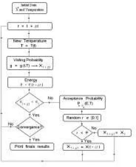
In order to make clear the procedure to construct the presently used computational code, we present the following owchart as Fig. 2:
Figure 2. Schematic diagram of Generalized Simulated An-nealing process.
II.3 Quantum Methodology: Density Functional
Embedded Cluster Scheme
The Density Functional (DF) theory is a standard tool for describing electronic structures, which is rst-principles in concept and exible in execution. DF the-ory has become a major tool for analyzing electronic structure of molecules and solids, with high intrinsic accuracy and reasonable computational eort. For ex-tended systems with no periodicity to exploit, a clus-ter approach oers many advantages, providing that a reasonable embedding scheme is used. Denition of 'reasonable embedding' depends upon the nature of the system- while a point charge environment is accept-able for a highly ionic compound, it is quite poor in
treating localized covalent interactions where there is hybridization of orbitals with neighboring atoms. The embedded cluster density functional (ECDF) scheme permits analysis of wavefunctions and their derived properties in a restricted volume, with interactions to the extended host included by eective potentials and boundary conditions. The present implementation of the ECDF scheme employs 'guard atoms' on the surface of the cluster to saturate interior bond structures, and synthesis of total charge and spin densities including the environment, to determine eective cluster poten-tials. Scanning algorithms by which the 'view window' of the cluster is moved over the volume of interest, per-mit treatment of extended systems. A key concept in obtaining self-consistency of the multiple overlapping views of a complex system like a heterogeneous inter-face, is that of equilibration of the chemical potential, or Fermi energy EF, among the component clusters. This methodology has been developed in several forms over the years, and successfully applied to a variety of molecules and extended solids, including metals, semi-conductors, and insulators; see for example [15].
In outline, the following main steps are performed in ECDF calculations:
i) Charge and spin densities of the extended sys-tem are constructed by summing component atom-like densities for the cluster and host:
( !
r) =
cluster+ host X
(13)
ii) LCAO-type basis functions are generated by nu-merical solution of DF equations for atoms/ions in a potential well, determined from the previous self-consistent-eld iterations; the basis is thus iterated as part of the overall optimization procedure.
iii) Form matrix elements of the eective Hamilto-nian
h =
t+V C+
V
and overlap operators over the AO basis j , pos-sibly transformed into symmetry orbitals, and orthog-onalized against a frozen core. Here t, VC , and VxC are kinetic energy, nuclear and electronic Coulomb po-tential, and exchange-correlation potential respectively. The index refers to spin orientation. The DF poten-tial is formed from the densities, and boundary condi-tions are applied to force localization of solucondi-tions to the cluster.
iv) Solve the Schrodinger (nonrelativistic) or Dirac (relativistic) equation, to obtain a variationalexpansion of the one-electron wavefunctions as
n ~ r) =
X j
j(
! r)C
j;n (15)
v) Project the cluster densities onto a localized 'ef-fective atom' expansion as
cluster= X
n f
n j
n j
2
=X
(16)
Here fnare Fermi-Dirac occupation numbers and enumerates atoms within the cluster.
vi) Analyze the interior `seed atom' region of each cluster to extract component atomic densities. New atomic densities for the next iteration are obtained after equilibration of the system and application of constraints such as electroneutrality of crystalline unit cells. Equilibrate the various clusters selected to span the region of interest, either by matching Fermi energies or spectral features, and iterate steps i-vi until adequate convergence of charge and spin distributions, spectral features, and total energy is obtained.
vii) Extract densities of states, optical and X-ray absorption coecients, electron energy loss spectra (EELS), cohesive energies, and other desired properties. Compare charge distribution and cohesive energies with data assumed in construction of MD/GSA potentials. Update MD/GSA potentials as required.
III Examples of Applications
Each of the components of the hybrid scheme: MD, MC/GSA, and ECDF have been developed indepen-dently and has a considerable history of successful ap-plications. The linkage between these components, with
the capability of feeding information between the com-ponents provides us with a powerful new tool for study-ing materials properties. An area of intense develop-ment in our laboratories is design and construction of a graphical user interface which will permit the use of this system of programs by non specialists, and particularly by experimentalists wishing to analyze new materials. In the remainder of this report, we give four illustra-tive examples related to current problems in materials design and optimization.
Beyond the general procedures outlined above, suc-cessful applications depend upon some degree of expe-rience and 'art'. For example; when is it most ecient to use MD and when is it better to use MC/GSA to de-termine the minimum-energy conguration of a system as complex as a ceramic grain boundary containing im-purities? In practical terms, we observe an initial rapid convergence with the MC/GSA approach, followed by a long 'tail' of sampling in which only small incremental improvements are found. Thus an optimal scheme in-volves switching from GSA to MD-gradient based pro-cedures at a rather well dened point in the simulation, when an accurate energy minimum is desired. Further details will be given elsewhere; here we only wish to comment briey on another important practical aspect: the use of boundary conditions and tight constraints to permit ecient sampling of regions of interest. In tradi-tional MD/MC one often tries to work with the largest possible simulation volume, to minimize boundary ef-fects, and distortions due to imposed periodicity. Here, we deliberately choose quite restricted simulation vol-umes, with tight boundary conditions, in order to focus upon system response to perturbations related to de-fects, surfaces, and interfaces. Of course, too tight con-trol completely prejudices the outcome of simulation, so convergence and stability tests have to be made as in any local scheme.
pa-rameters has to be considered. For example, in a typ-ical Born-type ionic interaction with point-charge long range terms, exponential repulsion, and inverse power short range attraction, modication of point charge val-ues also implies some modication of short-range pa-rameters to maintain correct bond lengths and cohesive energies.
I I I.1 ApplicationsUsinga CoupledDVM-GSA Metho d
I I I.1.1 A StackedLinearPorphyrinChain The chemical bonding of metal porphyrins, por-phyrazines, and phthalocyanines is of importance in understanding biophysical and catalytic processes. The crystalline materials like copper phthalocyanine (CuPc) form stacked chains, and when partially oxidized by io-dine (CuPcI) for example, become interesting 'molec-ular wire' conductors. Doped systems like Cu(1-x)Ni(x)PcI show quasi-one dimensional magnetic inter-actions of considerable theoretical interest. Component molecules (monomers) like CuPc are quasiplanar and small enough to be treated by standard quantum chem-ical approaches; however, understanding the electronic coupling between monomers requires a DF approach, and understanding the dynamics of coupling requires a MD/MC classical treatment. An ECDF/MD/MC study of a CuPc stack has been recently carried out [16]; here we wish to give a few highlights of the re-sults.
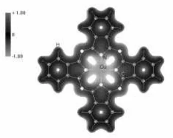
Fig.3 represents the electrostatic potential in a 3D-mapped isosurface of a porphyrin chain. The molecular equilibrium conformation was obtained using a GSA technique, coupled to a classical force eld. We have carried out semi- empirical Hamiltonian (PM3) calcu-lations to draw the electrostatic potential isosurface. One of the signicant conclusions drawn from this work is that standard force elds are capable of reproduc-ing both monomer and intermolecular interactions with considerable accuracy. Thus, while the underlying elec-tronic interactions (porphyrinic-ring pi versus metal-d; sigma bonding in-plane versus pi-interaction between molecules) are complex and require detailed analysis, a simple classical parametrization captures the main structural results. This observation helps to justify and motivate the mixed classical/quantum methodology.
Figure3. Electrostaticp otential ina3D isosurface.
Figure3a. Linearstacking ofaPorphyrinChain. I I I.1.2 Carb on InterstitialsinCopp er
is modied by the interfacial adsorption of the alloying elements which are added to the metal matrix.
High-resolution scanning electron microscopy (HRSEM) shows the existence of a 50nm solid so-lution zone at the copper-carbon interface, after an-nealing. After heat treatment of one hour at 1000 oC the interface faded and we can see a copper-carbon solid solution region of width 50 nm. Formation of a very dilute Cu-C interstitial solid solution at the interface may be diusion- controlled. To predict the diusion behavior of carbon atoms we have to study the structure and interatomic interactions in such alloys. Phenomenological studies of these phenomena have been augmented by quasi-continuum models [20] which reect some aspects of the underlying electronic struc-ture. Now the analysis is extended to the atomic scale, using a combination of GSA/MD atomistic simulations
and embedded cluster DF schemes.
Our MD simulations [20] are here deliberately con-strained to small displacements of the Cu host atoms, for which the framework of elastic Hooke's- law Cu-Cu interactions is quite adequate. As follows from sim-ple pseudopotential calculations, the Cu-C interaction is repulsive at least to several coordination shells sur-rounding the carbon atom. The repulsive part of in-teraction may be tted by any functional form, and we normally choose Lennard-Jones (LJ) parameters to re-produce the experimentally measured properties. Un-fortunately, experimental data on dilute Cu-C solid so-lutions are absent, so we use the results of the previ-ously mentioned pseudopotential studies.
The expression used for the classical system energy is thus
c E(r) = 12
X i;j
K ij(
r ij
,R 0ij)
2+ X i<j "
C 12(
i;j) r
12 ij
, C
6( i;j) r
6 ij
# +E
0
d The last term, E0, represents the volume-dependent part of the energy and includes information about elec-tronic density redistribution, which is gathered from the embedded cluster density functional scheme, or may be obtained from other electronic structure cal-culations. The parameter values are: R0=2.475A, K=6.920 eV/A2, E
0=-0.875 eV, C6=41.548 eV/A 6, C12= 2989.105 eV/A12.
Among the major conclusions of this work we nd the following:
i. Carbon strongly prefers the octahedral intersti-tial site over tetrahedral sites, as predicted from earlier works. We have determined the relative site energies and the (rather long range) relaxation of the Cu host around the impurity.
ii. Surface sites (incomplete octahedral interstitials) are at lower energy than volume sites, consistent with the extremely low solubility of C in Cu.
iii. Carbon dimers and hints of clustering appear at higher impurity densities.
iv. The graphite-Cu interface region appears to be disordered to a depth of several Cu atomic layers.
Figure 4. Two carbon atoms in a fcc-cell of Cu.One carbon atom is located in a substitutional position and the other one belongs to a tetrahedral interstitial position.
III.1.3 Scheelite, a Candidate Host for
Matrix-Fiber Composites
minerals of the same structure [22]. The WO4tungstate group exhibits strong bonding of mixed ionic and cova-lent character of great rigidity; as a result the scheel-ite lattice has a rather anisotropic response to pres-sure, with compression along the c-axis (see Fig. 5) being1.2 times that in the a-b plane. The W-O bond length is 1.75A ; in contrast, the Ca-O bond length is 2.41A and the Ca environment may be described best as an eight-fold coordinated cage, formed from oxygens of eight dierent surrounding WO4tetrahedra.
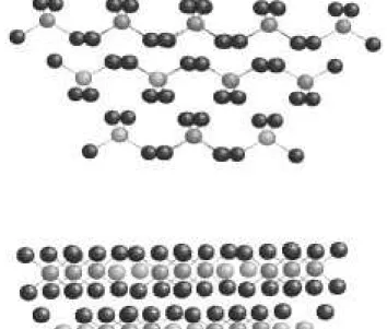
Figure 5. Lattice structure of scheelite.
The contrasting bond structures are the underly-ing reason for the apparently contradictory high melt-ing temperature and low fracture strength of the
ma-terial. These are precisely the characteristics which make scheelite interesting as a host matrix for ceramic matrix-ber composites (CFC). A useful CFC should be air stable to T >1300
oC, and under stress, crack-ing should take place in a controlled manner along the matrix-ber interface, allowing the bers to pull out and minimize structural damage. A typical ber can-didate would be-Al
2O3 and and so the surface struc-tures of scheelite and alumina, and their interfaces are of primary importance. Various crystallographic sur-faces of alumina have been characterized by experiment and theory; however, very little is known about the low energy surface structures of CaWO4. Simple consider-ations suggest that oxygen-terminated surfaces which preserve the WO4 units should be of relatively low en-ergy; thus we have carried out GSA modelling of the (001) oxygen terminated scheelite surface. A portion of the hemispherical (001) surface volume model is shown in Fig. 6; rigid embedding atoms included in the force eld are not shown.
Figure 6. Hemispherical dynamical volume representing scheelite (001) oxygen terminated surface in two dierent views.
rigidity of the WO4 structural unit. The expected re-sult is that the greatest response to crystal cleavage will be some rearrangement of the Ca ions with respect to the tungstate network. The surface relaxation energy is calculated to be 17 meV/A2with respect to the cleaved unrelaxed crystal, with tungstate angles held xed, and 20 meV/A2when exure is permitted.
The (001) oxygen-terminated cleavage plane, with its intact WO4groups, appears as the most obvious low energy surface. There are several other cleavage planes parallel to the c-axis which may be of relatively low energy. Interestingly, simulations of these surfaces by MD techniques suggest that cleavage along such places will result in spontaneous rupture along the (001) plane [23].
We have carried out ECDF calculations on the bulk and surface environments to determine major features of the electronic structure. The simplest analysis of the results can be made in terms of Mulliken atomic orbital populations and densities of states (DOS) dia-grams. In Table 2 we give the self-consistent orbital populations and charges for bulk and surface regions, noting that the formal valencies are Ca+2, w+6, O,2. Consistent with our qualitative discussion above, we see that calcium is near its nominal ionic value, indicating the relatively weak and long-range nature of its inter-actions. In contrast, the eective charge of +3 on tungsten emphasizes the covalent charge sharing in the (WO4)
2- group. As is generally found in metal oxides, the oxygen 2p band, while formally fully occupied, has in fact 0.5e vacancies per atom, due to charge transfer from the metals. The bonding-antibonding gap in en-ergy levels of the crystal-embedded (WO4)
2- complex is found to be 5.0eV, indicative of its great stabil-ity. The occupied valence band region shows W 5d, 6sp structures spanning 6eV and forming two distinct sub-bands with the O 2p, which can be qualitatively labeled as - and-type or equivalently denoted as e-and t- symmetry of the Td local point group.
In order to begin to explore the oxide-oxide in-terfaces critical for understanding matrix-ber inter-actions, we have generated a preliminary model for CaWO4 (001): MgO(001). To induce steps and irreg-ularities, the two surfaces have been made to intersect at an angle of 25 degress. The volume between the two perfect bulk crystals was 'regrown' using the GSA scheme with variable atomic composition and positions. ECDF studies were made of selected interface regions to examine rearrangement of electron densities
associ-ated with changes in coordination and bond lengths. A preliminary report on this work has been presented [24]; a detailed analysis of cohesion and bonding eects will be given elsewhere. A general conclusion that can be drawn from the surface and interface studies is that reduction in cation coordination and concomitant re-duction in average metal-oxygen bond lengths leads to reduced ionic charges at solid-vacuum and oxide-oxide interfaces. In the case of scheelite and related tetrahe-drally bonded materials like monazite, LaPO4, the ro-bust tungstate (phosphate) groups resist deformation and reduction processes, leading to special fracture be-havior and high temperature chemical stability.
Finally, we mention results of recent simulations on the scheelite (100): - Al
2O3 (0001) interface [23]. Rather large unit cells were used in slab geometry with two-dimensional periodicity, using a gradient-search MD scheme. It appears that relaxation is essentially localized to a few atomic layers on either side of the interface, due to the considerable rigidity of the Al-O and W-O bonds. The main relaxation mechanism is the rotation of the WO4groups to accommodate inter-face strain. ECDF calculations have been undertaken to verify the local electronic structure and to reconcile this structure with the force eld model.
III.2 Molecular Modeling in New Drug
Devel-opment
The development of a new pharmaceutical is a long and expensive process. A new compound must not only produce the desired response with minimalside- eects, but must be demonstrably better than existing thera-pies, and produced at a reasonable cost. Finding novel compounds with desirable properties can be a dicult problem, and one where molecular modeling has much to oer. The development of molecular modeling tech-niques is contributing to the understanding of biological processes at the atomic-molecular level and to the pro-posal of new molecular structures with high biological eciency. The action of many drugs, hormones and membrane proteins is dependent on the spatial con-formation adopted by the molecules in the inhomoge-neous environment formed by the cell membrane and its neighborhood.
understanding of the dynamic circumstances compati-ble with experimental observations, permitting a formal denition of the conditions that would be expected to
produce the observed behavior and therefore to infer patterns of behavior for situations of interest.
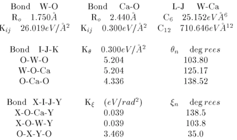
Bond W-O Bond Ca-O L-J W-Ca
Ro 1
:750A R
o 2
:440A C 6 25
:152eVA 6 Kij 26
:019eV=A
2 K
ij 0
:300eV=A
2 C
12 710
:646eVA 12
Bond I-J-K K 0
:300eV=A 2
n deg
r ees
O-W-O 5.204 103.80
W-O-Ca 5.204 125.17
O-Ca-O 4.336 138.52
Bond X-I-J-Y K (
eV=r ad 2)
n deg
r ees
X-O-Ca-Y 0.039 138.5
X-O-W-Y 0.039 103.8
O-X-Y-O 3.469 35.0
Table 1 - Hook's law, Lennard-Jones, Covalent bond angle, proper and improper dihedral parameters of GSA simulations for CaWO4
: Bulk Surface
W 5d 2.51 3.10
6s 0.08 0.06
6p 0.11 0.17
net charge 3.35 2.72
Ca 3d 0.03 0.02
4s 0.01 0.01
4p 0.06 0.04
net charge 1.92 1.94
O 2s 1.96 1.98
2p 5.33 4.88
net charge -1.29 -0.86
Table 2 - Self-consistent Mulliken atomic orbital pop-ulations and net atomic charges for dierent sites of (001) oxygen terminated scheelite.
III.2.1 Conventional Molecular Dynamics
Pro-cedure Applied to Biomolecular Systems
Our computationalcode, based on the classical force eld presented in section (2A), has an additional ca-pability of modeling molecules of biological interest in aqueous and apolar media, as well as at their inter-face. The software establishes two media with dier-ent continuous dielectric constants, separated by a cy-toplasm/membrane environment. The approach used to simulate the membrane interface is expressed by a discontinuity in the dielectric constant, taking into ac-count the dierent electrical polarizability of the aque-ous and the hydrocarbon phases. Then, the electro-static interaction between non bonded atoms at this
interface will be renormalized by the inuence of the di-electric discontinuity. The polarization eld produced at the surface of discontinuity by a point charge can be calculated by the method of images. A ctitious charge is placed in the opposite phase: the distance and the value of the image charge are xed by taking the ap-propriate electrical boundary conditions at the surface. When two charges i and j are on the same side of the interface, the potential on i due to j will have a contribution due to the image of j (i.e., j'), so that the Coulomb potential on i will be expressed by
V = 1 4 1
q ij
1 r
ij +
1 ,
2
1+
2 1 r
0 ij
! where
r ij =
(x
i ,x
j) 2+ (
y i
,y j)
2+ ( z
i ,z
j) 2
1=2
r 0 ij =
(x
i ,x
j ,2x
s) 2+ (
y i
,y j)
2+ ( z
i ,z
j) 2
1=2 and where rij and r
0
ij are the distance between i and j, and i and j' respectively. Xs is the position of the surface between the two media. When two charges are at dierent sides of the interface the method of image gives the following result:
Coli maltoporian [3],[4]. An important aspect of pep-tide simulation is the great number of degrees of free-dom for linear conformations, which can lead to sev-eral conformations with equivalent values of minimum energy. In this investigation we have studied a mutant signal sequence (78r1) of the LamB gene product, also called receptor or maltoporin, a protein of the exter-nal membrane ofE. coli. The mutant sequence contains
21 residues and shows a deletion of four residues in the hydrophobic region relative to the wild sequence. Such a deletion should abolish its capacity for helix formation and therefore its functionality. These eects were con-rmed experimentally. However, 50 was re-established by replacing a Gly residue with a Cys residue at residue 13 of the mutant peptide. The relevant sequences are
c
Wild type: MMITLRKLPLAVAVAAGVMSAQAMA
78r1 : MMITLRKLP|||VAAGVMSAQAMA
d Polarization eects on the peptide conformations have been investigated through the electrostatic charge image method as described above. A similar technique to simulate polarization eects in peptide conforma-tions has been proposed by some of the authors in Ref. [25]. These authors carried out a classical force eld simulation containing electrostatic image charge cal-culations to investigate the conformations of peptides characterized by dierent hydrophobicities at a water-membrane interface model. The interface is represented by a surface of discontinuity between two media with dierent dielectric constants, taking into account the dierence between the polarizabilities of the aqueous medium and the hydrocarbon one.
III.2.2 Stochastic Molecular Dynamics
Proce-dure Applied to Biomolecular Systems
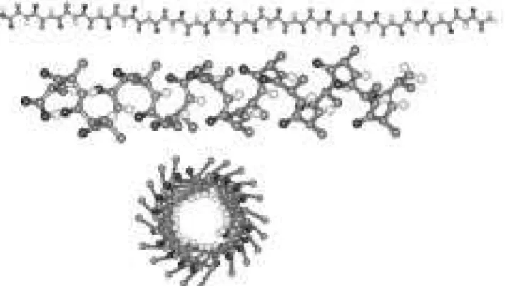
The biological function of a protein or peptide is often intimately dependent upon the conformation(s) that the molecule can be adopt. X-ray crystallogra-phy and NMR are two methods used to provide de-tailed information about protein structures. Unfortu-nately, the rate at which new protein sequences are de-termined experimentally is much greater than that for determination of structures. There is thus consider-able interest in theoretical methods for predicting the three-dimensional structure of a protein from its amino acid sequence; this is called the protein folding problem. Prediction of protein folding is a case where the usual MD is not a good theoretical method, since the real physical time of a folding process may be on the scale of minutes. To solve the time evolution of Newton's equation in MD it is necessary to discretize the time in
steps oft1 femtosecond, due to the intrinsic vibra-tional frequencies. This means that about 6x10¹⁶ MD steps would be needed to simulate the protein folding process, which is beyond computational possibility.
Figure 7. Ico-alanine p olyp eptid e in a linear- and helix-conguration.
IV Conclusions:
A nearly optimum procedure to search for minimum-energy structures is to initially scan using the MC/GSA scheme. As the slow-convergence region is attained, we switch to the MD/annealing scheme. The algorithms are coupled together in such a way as to permit this strategy, in a unied and convenient manner.
To extract electronic structure information in 'in-teresting' nuclear congurations, and not only in the state of lowest potential energy, we have the capacity to activate the Embedded Cluster Density Functional components of the codes from within the running dy-namics procedures. This permits generation of 'snap-shots' of electronic states during a process of molec-ular interaction or docking of a molecule with a sur-face, wall of a molecular sieve, or macromolecule. An important application which helps in dynamically re-parametrizing the interatomic potentials, is the deter-mination of atomic charges 'on the y'.
With the concept of self-consistent embedding, we have gained the ability to resolve large-size structures, containing thousands of atoms, and a size scale of at least 10 nm, as we have illustrated in the examples given here. Studies in progress on oxide surfaces, molecule-zeolite interactions, and grain boundaries in metals will help to determine future evolution of the hybrid
clas-sical/quantum procedure. Although GSA/MD/ECDF is already a powerful tool for the study of complex sys-tems, it is not optimized for processes which are essen-tially dynamic, such as diusion of atoms and molecules along interfaces and surfaces. It will be important to develop the capability for treating the longer time scales impliedby diusion processes; it is encouraging that the protein folding problem (which has a long time scale) has already been shown to be amenable to the GSA approach.
Graphical interfaces are essential now for controling and monitoring the models of complex systems. On the 'output side' we have various tools, which use commer-cial programs to visualize the results. Currently, we are working in the direction of increasing the `input side' to help the user dene and set up the model system.
Appendix
To generate the random vector x
tthe present GSA routine use an extension of the procedure used in ref-erence [12]. We have calculated the x=g
,1( !) us-ing a numerical integration of the visitus-ing distribution probability g
qV(
x). Where ! is a random vector [0,1] obtained from an equi-probability distribution andg
,1 is the inverse of the integral of g
q V(
x) given by c
g ,1(
!) =inv er se 0 @ x Z ,1 g q V( x)dx
1 A=
inv er se(!); (17)
g ,1(
!) =inv er se 0 B @ x Z ,1 q v ,1 1=2, 1, 1 2 (qv,1) qv,1 , 1 q v ,1 , 1 2 [T V q v( t)] , 1 3,qv f1 + (q
v ,1) (x) 2 [T V qv (t)] 2 3,q v g 1 q v ,1 , 1 2 dx 1 C A ; where qA (qV) is the
acceptanceindex (visiting index), and g
qv( 4x
t) = q v ,1 1=2, 1, 1 2 (q v ,1) qv,1 , 1 qv,1 , 1 2 [T V q v( t)] , 1 3,q v f1 + (q
v ,1) (4xt) 2 [T V q v (t)] 2 3,qv g 1 qv,1 , 1 2 : (18)
The integral ofg qV(
x) has an analytical solution only if (q
A; qV) = (1; 1) or (qA; qV) = (1; 2). For the general case it is necessary to make a numerical integration. In this paper,g
,1has been calculated using a series integration and taking the inverse of a polynomial series, whose expansion is cut o at the 17thorder.
The integral in equation 17 can be written as
!=!(x) = q v ,1 1=2, 1, 1 2 (q v ,1) qv,1 , 1 qv,1 , 1 2 x Z ,1 dx a (1 +bx
2)c
where a= [T V qv( t)] , 1 3,qv , b= (qv,1) [T V q v (t)] 2 3,qv
,c= 1 q v ,1 , 1 2 . Solving equation 19 using power series, we have;
!= 12 +ax, 1 3abcx
3
+ 15(12ac 2
b 2
+ 12acb 2)
x 5+
(20)
or
!(x) =! o+
A 1
x+A 2 x 3+ A 5 x 5+ =! o+ 1 X n=1 A n(
x,x o)
n (21)
We look for an inverse functiong ,1=
x=x(!) , such thatx(!),x= 0. From Eq.(21), we see that the inverse function may be expressed in terms of a power series,
x(!) =x o+ 1 X n=1 B n( !,! o) n : (22)
This is guaranteed by a theorem: Let!(x) be analytic at x=x o, and
d dx
!(x o)
6
= 0, then the inverse of !(x)
exists and is analytic in a suciently small region about!(x
o)and its derivative is 1 d dx
! (xo). The coecients B
n may be expressed in terms of A
n. However, it is possible to derive the coecients more elegantly by employing Cauchy's formula. In this case, B
ntakes the general form B
n= 1 nA n 1
X ; ;
(,1)
+ ++(
n)(n+ 1)(n,1 ++++) !! (A 2 A 1 )( A 3 A 1 ) (23)
The rst fewB
n coecients can be expressed as B
1 = 1 A 1 ; B 2= , A 2 A 3 1 ; B 3= 1
3A 3 1
" 34
2! A 2 A 1 2 , 3 1! A 3 A 1 # ; B 4= 1
4A 4 1
" ,
456 3! A 2 A 1 3 + 45
1!1! A 2 A 1 A 3 A 1 , 4 1! A 4 A 1 # : (24)
This last inversion was introduced in the GSA package, while the original proposition [11] uses a Levy-Flight distribution as the visiting distribution.
d References
[1] B.J. Alder and T.E. Wainwright, J. Chem. Phys. 27, 1208 (1957); Phys. Rev. 1, 18 (1970).
[2] N.L. Allinger and U. Burkert, \Molecular Mechanics", ACS-Monograph, 177(1982).
[3] E.P.G. Areas, P.G. Pascutti, S. Schreier, K.C. Mundim, P.M. Bisch, J. Phys. Chem.99, 14882 (1995).
[4] E.P.G. Areas, P. G. Pascutti, S. Schreier, K.C. Mundim, P.M. Bisch, Brazilian J. Mol. Biol. Res. 27,
527 (1994).
[5] S. Kirkpatrick, J. Stat. Phys.34, 975 (1984).
[6] S. Kirkpatrick, C.D. Gelat and M.P. Vecchi, Science 220, 671 (1983).
[7] D. Ceperly, C. Alder, Science231, 555 (1986). [8] H. Szu and R. Hartley, Phys. Lett. A122, 157 (1987). [9] C. Tsallis, J. Stat. Phys.52, 479 (1988).
[11] C. Tsallis and D.A. Stariolo, Phys. A233, 395 (1996). [12] K.C. Mundim, C. Tsallis, Int. J. Quantum Chem.58,
373 (1996).
[13] M.G. Moret, P.G. Pascutti, P.M. Bish and K.C. Mundim, J. Comp. Chem.19, 647 (1998).
[14] K.C. Mundim, T.J. Lemaire and A. Amin Bassrei, Physica A252, 405 (1998).
[15] D.E. Ellis and J. Guo, inElectronic Density Functional Theory of Molecules, Clusters, and Solids, ed. D.E. El-lis, (Kluwer, Dordrecht, 1995) p263.
[16] L. Guo, D.E. Ellis, K.C. Mundim and B.M. Ho-man, Journal of Porphyrins and Phthalocyanines 2, 1, (1998)
[17] S. Dorfman and D. Fuks, Composite Interfaces3, 431 (1996) and references therein.
[18] F. Dellanay, L. Froyen and A. Deruyttere, Journ. of Mater. Sci.22, 1 (1987).
[19] U. Gangopadhyay and P. Wynblatt, Journ. of Mater. Sci. 30, 94 (1995); S. Hara, K. Nogi and K. Ogino, in Proceedings of Int. Conf. \High-temperature capillar-ity".
[20] S. Dorfman and D. Fuks, Composites27A, 697 (1996). [21] D.E. Ellis, K.C. Mundim, D. Fuks, S. Dorfman and A. Berner, Mat. Res. Soc. Symp., Proc.527, 69 (1998). [22] H.W. Wycko, Acta Cryst.11, 199 (1958).
[23] C-K. Guo, D.E. Ellis, O. Warschkow, unpublished. [24] D.E. Ellis and K.C. Mundim, inProc. of 9th
CIMTEC-World Ceramics Congress Forum on New Materials, P. Vincenzine, Ed., Techna, Florence, 1998, to be pub-lished.
[25] P.G. Pascutti, K.C. Mundim, A. S. Ito and P.M. Bisch, J. Comp. Chem. (to be published 1999).