Abstract
One of the main drawbacks of Element Free Galerkin (EFG) method is its dependence on moving least square shape functions which don’t satisfy the Kronecker Delta property, so in this method it’s not pos-sible to apply Dirichlet boundary conditions directly. The aim of the present paper is to discuss different aspects of three widely used methods of applying Dirichlet boundary conditions in EFG method, called Lagrange multipliers, penalty method, and coupling with finite element method. Numerical simulations are presented to compare the results of these methods form the perspective of accuracy, conver-gence and computational expense. These methods have been imple-mented in an object oriented programing environment, called IN-SANE, and the results are presented and compared with the analyt-ical solutions.
Keywords
Element Free Galerkin method, EFG-FE Coupling, Lagrange Multipliers, Penalty Method, Object-Oriented Programming.
Imposition of Dirichlet Boundary Conditions in Element Free
Galerkin Method through an Object-Oriented Implementation
1 INTRODUCTION
Conventional numerical methods like Finite Element Method (FEM) are very powerful in solving different engineering problems, and they are efficiently being widely used through commercial software packages. But due to their reliance on mesh, these methods show limitations or difficulties when dealing with problems having large deformations or arbitrary path discontinuities.
Samira Hosseini a Mohammad Malekan a,* Roque L. S. Pitangueira a Ramon P. Silva a
aGraduate Program in Structural
Engi-neering (PROPEEs), School of Engineer-ing, Federal University of Minas Gerais (UFMG), Belo Horizonte, MG, Brazil [email protected],
[email protected], [email protected],
[email protected], [email protected]
* Corresponding author
http://dx.doi.org/10.1590/1679-78253607
Meshfree methods were introduced to eliminate part of those difficulties such as distorted ele-ments, need for re-meshing and the other limitations which arise because of element connectivity. A large variety of meshfree methods have been developed up to now for solving different engineering problems, such as smooth particle hydrodynamics (SPH) by Lucy (1997), diffuse elements, Nayroles et al. (1992), Element-Free Galerkin method (EFG), Belytschko et al. (1994), reproducing kernel particle method (RKPM), Liu et al. (1995), and hp-clouds methods, Duarte and Oden (1995).
Among introduced meshfree methods, element-free Galerkin is one of the most common methods which is based on the Moving Least Square (MLS) approximation, Lancaster et al. (1981). Since being introduced by Belytschko et al. (1994), this method has been used for solving different engineering problems like elasticity, static and dynamic fracture, Fleming et al. (1997), Belytschko et al. (1995a, 1196, 1997), Guiamatsia et al. (2009), manufacturing processes, Yonghui et al. (2008), and heat trans-fer, Singh et al. (2002).
The EFG method is a very promising method for the treatment of partial differential equations. Because of the absence of element connectivity, node particles can be added without the need for re-meshing, so adaptive refinement of the discretization can be performed easily. This makes the EFG method more flexible than finite element method, and prominent for solving problems involving large deformation, fracture and fragmentation. But EFG method still has some drawbacks compared with FE method. The most difficulties of this method are: 1) as a meshfree method, this method is also computationally expensive because of the complex meshfree interpolations and the complex imple-mentation algorithm, 2) since this method is based on the moving least squares shape functions, it is difficult to impose Dirichlet boundary conditions. Considerable researches have been devoted to over-come these difficulties, such as Lagrange multipliers method, Belytschko et al. (1994), and the penalty method Zhu and Atluri (1998), based on a modification of weak form. Other methods were proposed that can be interpreted as a modification of the interpolation shape functions, see for instance, Be-lytschko et al. (1995b), Huerta et al. (2000). The Lagrange multipliers method, firstly introduced by Babuška (1973), has been thoroughly studied by several researchers in Pitkäranta (1979), Barbosa et al. (1992), Stenberg (1995). This method is used to approximate the Dirichlet boundary conditions by using some unknown parameters called Lagrange multipliers. It was proven that this method had optimal convergence rates for the finite element spaces. The penalty method requires only the choice of the penalty parameter. The large values of this parameter must be used in order to impose the Dirichlet boundary condition in a proper manner. In practice, that might lead to ill-conditioned sys-tems of equations, reducing the applicability of this method. Further information on penalty method can be found in Zhu and Atluri (1998).
proposed by Belytschko[14]. Another approach for coupling EFG and FE is by using Lagrange mul-tipliers. In this approach the substitution of FE nodes by particles is not necessary, Hegen (1996), Rabczuk and Belytschko (2006). Another coupling approach using Lagrange multipliers was proposed by Belytschko and Xiao, called ‘bridging domain coupling method, Belytschko and Xiao (2004). In their approach, FE nodes and meshfree particles could overlap. Gu and Zhang (2008) developed a new concurrent simulation technique to couple the EFG method with the finite element method for the analysis of crack tip fields, using the ‘bridging domain coupling method’ concept and Lagrange multipliers. Liu et al. (2008) presented an adaptive EFG-FE coupling method oriented for bulk metal forming. In their method the simulation is performed using finite elements initially. During the pro-cess, the FE region with severe deformation occurrence is automatically converted to an EFG region.
The application of FEM object-oriented programming has been receiving great attention over the last two decades. As a result, a bunch of FEM-based codes used object-oriented concept as their implementation strategy, such as: a C++ based finite element code developed by Patzak et al. (2001), a meshless Object-oriented programming (OOP) code using non-uniform rational b-spline, Zhang et al. (2006), Freefem++, Hecht (2012), a fem code to solve two- and three-dimensional problems, a general framework for weak-form meshfree methods by Hsieh et al. (2014), and an educational FE software for truss structures presented by Zou et al. (2014).
In the present work, the three introduced methods of applying Dirichlet boundary conditions are investigated through developing MATLAB codes and also implementation of an object-oriented pro-gramming environment, called INSANE (INteractive Structural ANalysis Environment- http://www.insane.dees.ufmg.br) platform, Alves et al. (2013), Fonseca and Pitangueira (2007). The main contribution of the present work is regarding to implementation which, to the best knowledge of the author, is the first object oriented program for meshfree methods and also EFG/FE coupling approach. The implemented EFG program is highly efficient with a wide range of applications since it' s built on the basis of a well-developed finite element program, not only in the sense of using integration cells but, indeed the ability of using several features of FEM code which are already implemented, or will be further implemented in INSANE computational platform. The most signifi-cant example for this is the capability of using existing physically nonlinear models of FEM code, such as smeared crack and damage models in order to solve continuum damage problems in meshfree framework. This paper is arranged as follows: first a brief review of EFG formulation will be presented, and the methods of applying Dirichlet boundary conditions which are studied in this work will be explained. Then the INSANE platform will be briefly introduced with emphasis on its meshfree mod-ules. In Sect. 5 the numerical examples will be presented and the results will be compared with the analytical solutions.
2 ELEMENT FREE GALERKIN METHOD
2.1 Moving Least Square Approximation
1
( )
m( ) ( )
( ) ( )
h T
i J iJ i
J
u
p
a
x
x
x p x a x
(1a)where p(x) is a complete polynomial basis of arbitrary order and are coefficients which are
obtained at any point x by minimizing the following:
2 1
(
)
( ) ( )
sn n T I iI I i IJ
w
u
x x
p x a x
(1b)in which nsn is the number of nodes in the support domain of point x, and w(x-xI) is considered as a
cubic spline weight function defined by:
2 3
2 3
2
4
4
1
2
3
4
4
1
( )
4
4
2
1
3
3
0
1
r
r
for r
w r
r
r
r
for
r
for r
(2)Minimizing Eq. (1b) leads to:
1
( )
( ) ( )
i
x
x
i
a x A
B u
(3)where:
1
( )
nsn(
) ( ) ( )
TI I I
I
w
A x
x x p x p x
(4)and,
1 1 2 2
( )
w
(
) ( ), (
p
w
) ( ), , (
p
w
n) ( )
p
nB x
x x
x
x x
x
x x
x
(5)
1, , ,
2
T
i
u u
i iu
inu
(6)By substituting Eq. (3) into Eq. (1a), the MLS approximants are defined as:
1
( )
nsn( )
h
i I iI
I
u
u
x
x
(7)where ∅ are the EFG shape functions and are defined as:
1
1
( )
m( )
( ) ( )
I J JI
J
p
2.2 EFG with Lagrange Multipliers
For any trial function, ∈ , and test function, ∈ , the Galerkin weak form of the EFG method
with Lagrange multipliers is:
.
(
)
0
g h
g
k v
ud
v d
v fd
vhd
v
U
r u
g d
r
U
(9)with the following boundary conditions:
0 .
g
h
u g on
k u h on
n
where U and S are the spaces of test and trial functions, respectively, Γ and Γ are the Dirichlet
and Neumann boundaries, is Lagrange multiplier, and f is the excitation vector.
Applying the moving least square approximations (Eq. (7)), the resulting system of equations for EFG method with Lagrange multipliers is:
T
K G u
f
G
0 λ
q
(10)where:
.
h
g
g
IJ I J
I I I
IK I K
K K
K
k
d
f
f d
hd
G
N d
q
N gd
(11)As can be seen in Eq. (10), this method introduces additional unknown variables, , which results in a larger system of equations compared with FEM, which means increasing the computa-tional cost.
2.3 EFG with Penalty Method
The Galerkin weak form for EFG with penalty method is:
. ( )
g h
k v ud
v u g d v fd vhd v U
in which is the penalty parameter used to apply Dirichlet boundary condition. Using MLS approx-imation leads to the following system of equations:
K K U f f
(13)where:
.
g
h
g
IJ I J
IJ I J
I I I
I I
K
k
d
K
d
f
f d
hd
f
gd
(14)
This method produces a system of equations with the same dimensions of FEM, but choosing the proper value for the penalty parameter is critical for this method. Penalty parameter should be as large as possible, but not too large to produce numerical problems due to increasing the condition number of the system matrix.
2.4 EFG Coupled with FEM
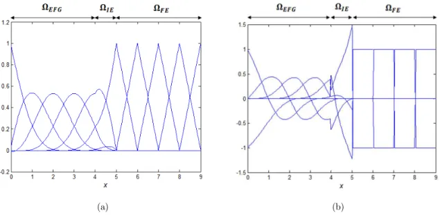
In order to couple EFG with FEM using ramp function, Belytschko et al. (1995b), domain of the problem is divided into three subdomains, as shown in Figure 1.
In Ω , the solution value at each point is approximated using the MLS approximants as in Eq.
(7). In Ω , the standard finite element interpolation functions are used to approximate the solution,
and in Ω which the interface elements are located, the following expression is used:
( )
( )
( )
( )
( )
1
( )
( )
( )
( ) ,
h FE EFG FE FE EFG
i i i i i i IE
u
x
u
x
R
x
u
x
u
x
R
x
u
x
R
x
u
x
x
(15)where and are approximations for u in Ω given by the FE and EFG approximations,
respectively, and R(x) is the ramp function defined by Belytschko et al. (1995b):
1
( )
J EFG J J xR
N
x
(16)In other words, the ramp function is equal to the sum of the FE shape functions of interface element nodes that are on the EFG boundary. By substituting the FE and EFG solution approxima-tions in Eq. (15) it obtains:
1 1 1
( ) 1
( )
nne( ( ))
( )
nsn( )
nsn( )
,
h e
i I iI I iI I iI IE
I I I
u
R
N
u
R
u
N
u
x
x
x
x
x
x
x
(17)which the are the shape functions of nodes of interface elements and are defined by [14]:
1
( )
( ( ))
( ) ( )
( )
( ) ( )
e
I I I IE
I e
I I IE
R
N
R
N
R
x
x
x
x x
x
x
x
x
(18)And the derivatives of the shape functions are:
, , , ,
,
, ,
1
( )
( )
( )
( )
e i I I i i I I i I IE
I i e
i I I i I IE
R N
R N
R
R
N
R
R
x
x x
x
x
x
(19)(a) (b)
Figure 2: Coupled Shape functions in 1-D: (a) Shape function, (b) Shape function derivative.
(a)
(b) (c)
Figure 3: Coupled shape functions in 2-D: (a) Shape function, (b) Shape function derivative with respect to x, (c) Shape function derivative with respect to y.
0 1 2 3 4 0
1 2
3 4 -0.1
0 0.1 0.2 0.3 0.4 0.5 0.6
x y
0 1 2 3 4 0
2
4 -0.6
-0.4 -0.2 0 0.2 0.4 0.6 0.8 1 1.2
x y
0 2
4
0 1
2 3
4 -0.5
0 0.5
3 INTERACTIVE STRUCTURAL ANALYSIS ENVIRONMENT (INSANE)
The INSANE environment is an open source software implemented in Java, an OOP language. It is composed of three main applications: pre-processor, processor and postprocessor. The pre- and post-processor are interactive graphical applications that provide tools to build representations of the structural problem as well as its results visualization. The processor is the numerical core of the system, responsible for obtaining the results of the analysis. There are different computational meth-ods available for the processor, such as FEM, Fonseca and Pitangueira (2007), Generalized/Extended FEM, Alves et al. (2013), Malekan and Barros (2016), Malekan et al. (2016a, 2016b, 2017), and Boundary element method, Anacleto et al. (2013), Peixoto et al. (2016).
3.1 Main Structure
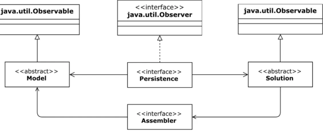
The numerical core of INSANE is composed of two interfaces: Assembler, and Persistence and two
abstract classes: Model and Solution. Figure 4shows the Unified Modeling Language (UML) form of
the numerical core.
Figure 4: Organization of numerical core of INSANE.
The Assembler interface builds the matrix of system of equations given by the discretization of a boundary or initial value problem, being implemented with following general representation:
AX + BX + CX = D (20)
Where X is the solution vector; A, B and C are matrices and D is a vector, where may or may not
be dependent on the state variable or its derivatives.
Solution class has the necessary methods for solving the matrix system of Eq. (20), and the Model
abstract class contains the data of the discrete model and provides Assembler with all necessary
information to assemble Eq. (20).
Both Model and Solution communicate with the Persistence interface, which treats the input data
and persists the output data to the other applications, any time it observes a modification of the
pattern, Horstmann et al. (2008). In this mechanism when an object of type observer (which imple-ments the interface java.util.observer) is created, it will be added to a list of observers and will have a list of observables (which extends the class java.util.observable). In case of any modification in the state of any observable object, the change propagation mechanism is triggered, and the observer objects are notified to update themselves. This process guarantees the consistency between the
ob-server and the observed components. In INSANE, the obob-server component is Persistence and the
observed components are Solution and Model abstract classes.
3.2 Assembler
The MfreeAssembler class has the necessary methods for assembling the matrix system of the Eq. (20), with three ways to apply essential boundary conditions: coupling with finite element method, using the method presented in Fernández-Méndez et al. (2004), Lagrange multipliers, and penalty method. In static analysis using penalty method or EFG-FE coupling technique, the matrix system of equations is:
uu up u p
pu pp p u
C C X D
C C X D (21)
where the matrix C represents the stiffness matrix of the model, X is the vector of nodal parameters,
and D is the vector of forces. The indices u and p indicate unknown and prescribed values,
respec-tively.
In static analysis using Lagrange multipliers the system of equations to be solved is:
uu u p
T
C
G X
D
G
0
λ
q
(22)This class has methods to build different parts of the matrix system, according to Eq. (21) and
Eq. (22). The organization of the classes which implement the Assembler interface is illustrated in
Figure 5. In this figure the UML diagram of the MfreeAssembler is showing the main methods of
this class.
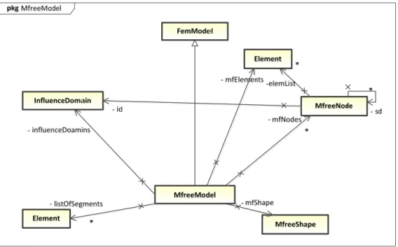
3.3 Model
The objective of the Model abstract class is to represent the discrete model of the problem. It is
implemented by the object of class FemModel which itself consists of objects of different classes
specifying the attributes of the model.
Figure 6 shows the UML diagram of the MfreeModel class and its related classes. MfreeModel uses
Figure 5: Organization of Assembler interface.
3.4 Solution
The abstract class Solution, manages the solution process of solving matrix system of Eq. (20). In
case of linear static problem a class named SteadyState implements the class Solution.
Each object of type SteadyState has attributes of two other objects of type Assembler and
Line-arEquationSystems .The class LinearEquationSystems has different methods for standard techniques of solving linear equation systems. This class receives the matrix system of equations (Eq. (20)) built
by class Assembler, and computes the solution vector. For solving a linear static meshfree problem
this class returns the vector of nodal values.
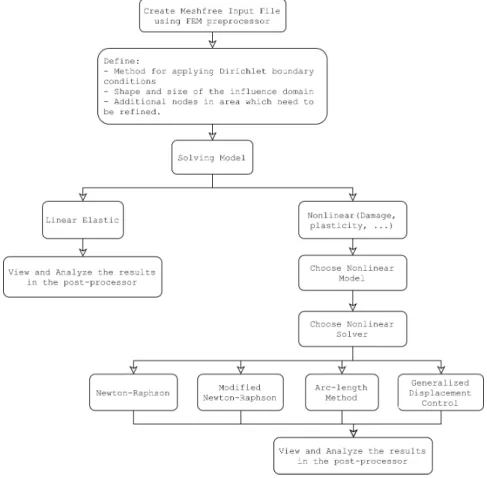
3.5 Analysis Flowchart
Figure 7 shows a detailed flowchart for meshfree analysis described in this section. The process starts with creating a meshfree input file, then defining analysis parameters such as size and shape of the influence domain. Two types of solution procedures are available, either linear elastic or nonlinear analysis. Following selection of the solver type, the problem will be solved and user can work on the results using the available post-processor part. Similar flowchart can be drawn for EFG/FE coupling approach, except the coupling domain have to be defined before solving the model.
4 NUMERICAL RESULTS
In order to investigate the difference between the methods of applying Dirichlet boundary conditions in EFG method, two well-known cases are studied: Timoshenko beam and Laplace equation. A com-putational code is developed in order to solve these problems with EFG meshfree method, using the three previously mentioned methods to apply Dirichlet boundary conditions. The case of Timoshenko beam is also implemented in INSANE platform.
4.1 Cantilever Beam
For a Timeshenko beam as an elastostatic problem, the differential equation is as follows:
.
0
u
j j t
b
in
u u on
n
t on
(23)
In which is the body force, , and , Γ and Γ are the essential and traction
bound-aries, respectively. The resulting system of linear equations is:
ku f
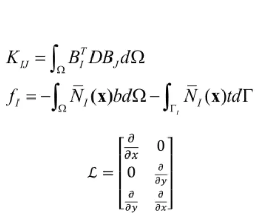
(24)in which:
( )
( )
t
T IJ I J
I I I
K
B DB d
f
N
bd
N
td
x
x
(25)(26)
The model of the cantilever beam is illustrated in Figure 8. The following parameters are consid-ered for the model: L=48, D=12, E=30e6, =0.3, and P=-1000.
Regular meshes were used, with 4 × 4 quadrature in each EFG cell and also for the coupled FE
elements. A linear basis was used for EFG and standard Q4 elements were used in Ω .
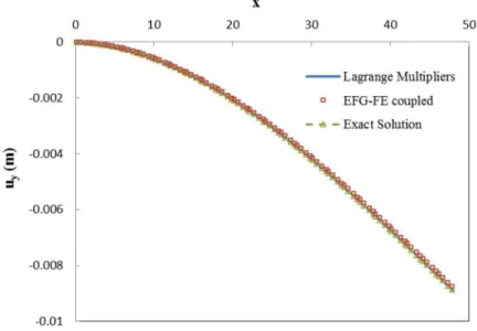
Figure 9: Deflection of Timoshenko beam in y direction.
Two cases are investigated for coupled EFG-FE problem. In the first case, the left half of the beam is modeled using FE elements, and the right half by EFG nodes. In the last strip of the FE domain the interface elements are located. The results for the deformation of the beam, in the y direction are illustrated in Figure 9 and are compared with Lagrange multipliers and analytical solu-tion. The exact solution for the vertical displacement of Timoshenko beam is:
2
2 2
3 ( ) (4 5 ) (3 )
6 4
y
P D x
u y L x L x x
EI
(27)
where I is the moment of inertia for a beam with rectangular cross-section and unit thickness.
In the second case only a strip of the interface elements is located in the position of Γ and the
remaining parts of the beam are modeled by EFG nodes. This strip of interface elements makes it possible to impose the essential boundary condition accurately.
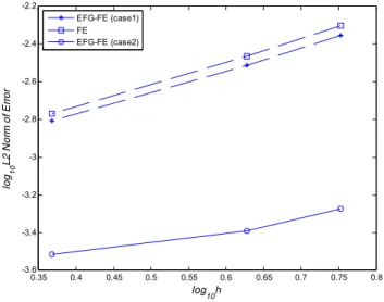
The L2 norm of error for the displacement in the y direction is obtained from the Eq. (28) and
compared for the two cases, and with the FE results in Figure 10. In this figure h is the distance
between the nodes.
2
1 2
(
h exact T) (
h exact)
L
E
u
u
u
u
d
(28)Figure 10: Variations of error versus mesh size, for 36, 64, and 240 nodes.
The Central Processing Unit (CPU) times of the solution for these two cases are compared with each other and with FE in Figure 11. As can be expected, case 2 involves the largest CPU time (because of the larger number of meshfree particles), but in cases of coarser nodal distributions, it has resulted in better accuracy, using almost the same CPU time.
The results of solving Timoshenko beam problem with INSANE software are illustrated in Figure 12 for vertical displacements of points on the beam’s mid-plane. Regular meshes were used, with 5 × 5 quadrature points in each EFG cell and also for the coupled FE elements. A linear basis was used
for EFG and standard eight-node quadrilateral (Q8) elements were used in Ω in order to use
EFG-FE coupling method. Only a strip of interface elements are placed at Γ and also at x=L, where the
load is applied. The results show a very promising accuracy even using a coarse nodal distribution.
Figure 11: Variation of CPU time versus error, for 36, 64, and 240 nodes.
0.35 0.4 0.45 0.5 0.55 0.6 0.65 0.7 0.75 0.8 -3.6
-3.4 -3.2 -3 -2.8 -2.6 -2.4 -2.2
log
10h
lo
g10
L2 N
or
m
of
E
rr
or
EFG-FE (case1) FE EFG-FE (case2)
0 2 4 6 8 10 12 14 16
-3.6 -3.4 -3.2 -3 -2.8 -2.6 -2.4 -2.2
CPU time
lo
g10
L2 N
or
m
o
f E
rr
or
Figure 12: Deflection of Timoshenko beam in y direction using INSANE implementation.
4.2 Laplace's Equation with Mixed Boundary Conditions
The second numerical example is the Laplace's equation with mixed boundary conditions on a rec-tangle. The differential equation for this problem is:
, , ∈ , , ∈ ,
( ,0) 0 (0, ) 0
( ,10) 100sin 10
(5, ) 0
u x u y
x u x
u y x
(29)
The analytical solution for this problem is:
100sin( )sinh( )
10
10
sinh( )
x
y
u
(30)In order to investigate the EFG-FE coupling results in this problem only a strip of interface elements are located at the essential boundary locations, as shown in Figure 13.
The obtained solutions over the whole domain are demonstrated in figures 14-16 for EFG-FE
coupled, Lagrange multipliers and penalty method ( ). The absolute values of error are shown
Figure 13: Domain discretization for Laplace problem.
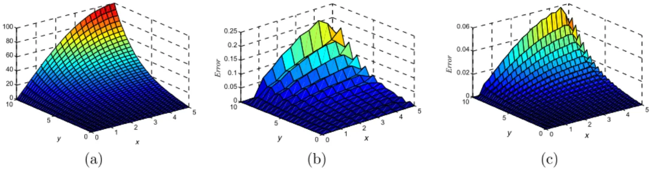
(a) (b) (c)
Figure 14: Solution of Laplace equation using EFG-FE coupling method, a) solution, b) absolute error of approximation using 200 nodes, c) absolute error of approximation using 800 nodes.
(a) (b) (c)
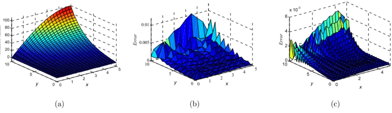
Figure 15: Solution of Laplace equation using Lagrange multipliers, a) solution, b) absolute error of approximation using 200 nodes, c) absolute error of approximation using 800 nodes.
0 1 2 3 4 5 0 5 100 20 40 60 80 100 x y so lu tio n va lu es 0 1 2 3 4 5 0 5 100 0.05 0.1 0.15 0.2 0.25 x y Er ro r 0 1 2 3 4 5 0 5 100 0.02 0.04 0.06 x y E rr o r 0 1 2 3 4 5 0 5 10 0 20 40 60 80 100 x y so lut io n v a lue s 0 1 2 3 4 5 0 5 100 0.005 0.01 0.015 x y E rro r 0 1 2 3 4 5 0 5 100 1 2 3 4
x 10-3
x y
Er
ro
(a) (b) (c)
Figure 16: Solution of Laplace equation using penalty method, a) solution, b) absolute error of approximation using 200 nodes, c) absolute error of approximation using 800 nodes.
In Figure 14, the values of error are equal to zero at Dirichlet boundaries. Comparing these three figures, penalty method shows the largest error at Dirichlet boundaries. On the other hand, by in-creasing the number of nodes, the error of approximation at Dirichlet boundaries using Lagrange multipliers shows more significant decrease than the penalty method.
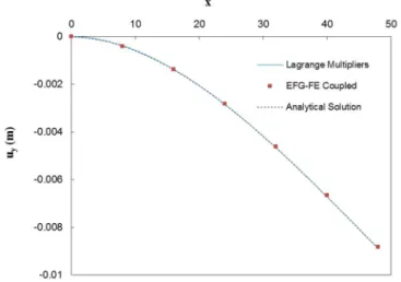
Figure 17: Values of solution for Laplace equation at x=5.
The values of solution at Neumann boundary of domain, x=5, are compared with the analytical
solution in Figure 17 for three methods of Lagrange multipliers, penalty, and EFG-FE coupling.
4.3 Effect of Penalty Parameter on Convergence
For the case of Timoshenko beam the logarithmic values of energy norm against nodal spacing, h, are
plotted in Figure 18. This plot is obtained using the EFG method for different penalty parameters,
8. The nodal spacing was chosen from h = 0.25 to h = 0.1.
0 1 2 3
4 5 0
5 10
0 20 40 60 80 100
x y
so
lut
ion
v
a
lues
0 1 2
3 4 5
0 5 100 0.005 0.01
x y
E
rro
r
0 2 4 0
5 100
2 4 6
x 10-3
x y
Er
ro
Figure 18: Energy norm against nodal spacing for Timoshenko beam
using different penalty parameters, .
It is clearly seen that the error in energy norm for penalty parameter is less than the
other cases, so, this value has been used for obtaining EFG results and been compared with other approaches like Lagrange multipliers and EFG-FE coupling.
Figure 19 compares the rate of convergence considering different values of nodal spacing, h, for
the solution of Timoshenko beam using EFG method based on two different approaches in order to apply Dirichlet boundary conditions: Lagrange multipliers method and penalty method. In this figure, the convergence rate of EFG approximation using Lagrange multipliers and penalty method are about 0.94269 and 1.1762, respectively, which shows that EFG solution with penalty method converges faster than EFG with Lagrange multipliers.
L2-norm of error against nodal spacing for the 2D Laplace problem is illustrated in Figure 20. This figure contains L2-norm for different approaches, like FE, EFG using Lagrange multipliers, EFG
using penalty method (for and ) and EFG-FE coupling approach. Although the rate
of convergence for FE method, EFG using Lagrange multipliers method and EFG-FE coupled method are the same (equal to 1.99), but the error in L2-norm for EFG using Lagrange multipliers is less than the other two methods. In addition, it can be seen that EFG using penalty method with
shows the best results considering both convergence rate (equal to 4.449) and the accuracy.
Figure 20: Rate of convergence in energy norm for the 2D EFG
problem using Lagrange and penalty ( ) methods.
5 CONCLUSION
Future studies will focus on solving nonlinear problems such as damage propagation using meshfree part of the INSANE computational platform. In addition, the implemented meshfree pro-gram could also communicate with the GFEM module of the INSANE code, and using the imple-mented enrichment functions and methods of treating crack singularities in those classes, become an extended EFG (XEFG) method and be able to explicitly model the problems with discrete crack propagation in structures; which the last two aspects are also the subjects of ongoing works of the authors.
Acknowledgments
This research is funded by Brazilian research agencies CNPq (National Council for Scientific and Technological Developments - Grant 308785/2014-2), FAPEMIG (Foundation for Research Support of the State of Minas Gerais - Grant PPM-00669-15) and CAPES (Coordination for the Improvement of Higher Education Personnel).
References
Alves P.D, Barros F.B, Pitangueira R.L.S (2013) An object oriented approach to the generalized finite element method. Advances in Engineering Software, 59: 1–18.
Anacleto F.E.S, Ribeiro T.S.A, Ribeiro G.O, Pitangueira R.L.S, Penna S.S. (2013) An object-oriented tridimensional self-regular boundary element method implementation, Engineering Analysis with Boundary Elements 37(10):1276– 1284
Babuška I. (1973) The finite element method with Lagrange multipliers. J. Numerical Mathematics 20: 179–192. Barbosa H.J.C, Hughes T.J.R. (1992) Boundary Lagrange multipliers in finite element methods: error analysis in natural norms. J. Numerical Mathematics 62: 1–15.
Belytschko T, Lu Y. Y, Gu L. (1994) Element-free Galerkin methods. Int. J. Numerical Methods in Engineering 37: 229-256.
Belytschko T, Lu YY, Gu L. (1995a) Element-free Galerkin methods for static and dynamic fracture, Int. J. of Solids and Structures 32: 2547–70
Belytschko T, Organ D, Krongauz Y. (1995b) A coupled finite element-element-free Galerkin method. Computational Mechanics 17: 186–195.
Belytschko T, Xiao SP. (2004) A bridging domain method for coupling continua with molecular dynamics. Computer Methods in Applied Mechanics and Engineering 193: 1645–1669.
Belytschko T., Tabbara M. (1996) Dynamic fracture using element-free Galerkin methods. Int. J. Numerical Methods in Engineering 39: 923–38.
Duarte C. A, Oden J. T. (1995) Hp clouds - a meshless method to solve boundary-value problems. Technical Report, Texas Institute for Computational and Applied Mathematics, University of Texas at Austin, 95-105.
Fernández-Méndez S, Huerta A. (2004) Imposing essential boundary conditions in mesh-free methods. Computer Meth-ods in Applied Mechanics and Engineering 193: 1257-1275.
Fleming M, Chu YA, Moran B, (1997) Enriched element-free Galerkin methods for crack-tip fields. Int. J. Numerical Methods in Engineering 40: 1483–504.
Fonseca F.T, Pitangueira R.L.S (2007) An object oriented class organization for dynamic geometrically non-linear. CMNE (Congress on Numerical Methods in Engineering)/CILAMCE 2007, Porto, 13-15 June, Portugal
Guiamatsia I, Falzon B.G, Davies G.A.O, (2009) Element-Free Galerkin modeling of composite damage. Compos. Sci. Technol. 69: 2640–648.
Hecht F., (2012) New development in freefem++. Journal of Numerical Mathematics 20(3-4): 251–265.
Hegen D. (1996) Element free Galerkin methods in combination with finite element approaches. Computer Methods in Applied Mechanics and Engineering 135: 143–166.
Horstmann CS, Cornell G. (2008) Core java – fundamentals, vol. 1, 8th ed. Sun Microsystems Press.
Hsieh Y-M, Pan M-S (2014) ESFM: An essential software framework for meshfree methods. Advances in Engineering Software 76: 133–147.
Huerta A, Fernandez-Mendez S. (2000) Enrichment and coupling of the finite element and meshless method. Int. J. Numerical Methods in Engineering 48: 1615 1636.
Krongauz Y, Belytschko T. (1996) Enforcement of essential boundary conditions in meshless approximations using finite elements. Computer Methods in Applied Mechanics and Engineering 131: 133-145.
Lancaster P, Salkauskas K, (1981) Surface generated by moving least square methods. J. Computational Mathematics 37: 141–58.
Liu L.C, Dong X.H, Li C.X. (2008) An Adaptive EFG-FE Coupling Method for the Numerical Simulation Of Extrusion Processes. Acta Metallurgica Sinica (English Letters), 21: 380-388.
Liu W. K, lun S, Li S, (1995) Reproducing kernel particle methods for structural dynamics. Int. J. Numerical Methods in Engineering 38: 1655-1679.
Lucy L. B (1997) A numerical approach to the testing of fission hypothesis. The Astronomical Journal 82: 1013–1024. Malekan M, Barros F.B, Pitangueira R.L.S, Alves P.D (2016a) An object-oriented class organization for global-local generalized finite element method. Latin American Journal of Solids and Structures 13(13):2529–2551.
Malekan M, Barros F.B, Pitangueira R.L.S, Alves P.D, Penna S.S (2017) A computational framework for a two-scale generalized/extended finite element method: generic imposition of boundary conditions. Engineering Computations, 34(3), pp 1–32.
Malekan M, Barros F.B, Silva R.P, (2016b) Development and implementation of a well-conditioning approach toward generalized/extended finite element method into an object-oriented platform. Revista Interdisciplinar de Pesquisa em Engenharia 2(14):1-20.
Malekan M, Barros FB (2016) Well-conditioning global-local analysis using stable generalized/extended finite element method for linear elastic fracture mechanics. Computational Mechanics 58(5): 819-831.
Nayroles B, Touzot G, Villon P. (1992) Generalizing the finite element method: diffuse approximation and diffuse elements. Computational Mechanics 10: 307-318.
Patzaak B., Bittnar Z., (2001) Design of object oriented finite element code. Advances in Engineering Software 32: 759-767.
Peixoto R.G, Anacleto F.E.S, Ribeiro G.O, Pitangueira R.L.S (2016) A solution strategy for non-linear implicit BEM formulation using a unified constitutive modelling framework, Engineering Analysis with Boundary Elements, 64:294-310.
Pitkäranta J. (1979) Boundary subspaces for the finite element method of Lagrange multipliers. J. Numerical Mathe-matics 33: 273–289.
Rabczuk T, Belytschko T. (2006) Application of mesh free methods to static fracture of reinforced concrete structures. Int. J. Fracture 137(1–4): 19–49.
Singh I.V, Sandeep K, Prakash R. (2002) The element free Galerkin method in three dimensional steady state heat conduction. Int. J. Computational Engineering Science 3(3): 291-303.
Yonghui L., Jun C., Song Y. (2008) Numerical simulation of three-dimensional bulk forming processes by the element-free Galerkin method. Int. J. Advanced Manufacturing Technology 36(5): 442-450.
Zhang X., Subbarayan G, (2006) jNURBS: An object-oriented, symbolic framework for integrated, meshless analysis and optimal design. Advances in Engineering Software 37: 287–311
Zhu T., Atluri S.N. (1998) A modified collocation method and a penalty formulation for enforcing the essential bound-ary conditions in the element free Galerkin method. Computational Mechanics 21(3): 211–222.
Zou W., Li X., Guo G. (2014) EFESTS, Educational finite element software for truss structure. Part I: Preprocess. International Journal of Mechanical Engineering Education 42(4): 298–306.