Lat. Am. j. solids struct. vol.14 número6

Abstract

As extension of the previous two-surface model in plasticity, a two-surface model for viscoplasticity is presented herein. In order to validate and investigate the performance of the proposed model, several numerical simulations are undertaken especially for struc-tural steel under monotonic and cyclic loading cases, where exper-imental results and numerical results from the rate dependent kinematic hardening model are also provided for the reference. For all the cases studied, the proposed model can appropriately ac-count for the rate-effects in both maximum stress and hysteretic shapes.

Keywords

Two-surface model; Viscoplasticity; Numerical simulation.

A Two-Surface Viscoplastic Model for the Structural Steel

1 INTRODUCTION

The general description of material nonlinearity primarily concerns a constitutive equation. Essen-tial ingredients to establish this constitutive equation can be characterized by yield surface (or yield stress function), plastic flow rule, normality rule and hardening law- the yield surface divides the elastic and plastic region; the flow rule relates the plastic strain to stress state; the normality rule leads the incremental plastic strain to the normal level of the yield surface; the hardening law de-scribes the plastic evolution. While the classical rate independent plasticity (so called plasticity) is often illustrated by a single yield surface with either isotropic hardening or kinematic hardening, these models can not completely express the hardening behavior of material. In particular, in the single yield surface model, the elastic domain is considered to be too large compared to experiment results and it is difficult to describe sudden changes from elastic to plastic or plastic to elastic region (Chaboche (2008)). Also, it cannot solely account for cycle-by-cycle accumulation of permanent deformation (ratcheting), which often happen in engineering practice (Bari and Hassan (2008)). In order to account for more realistic response of plasticity, previously, two-surface and multiple yield

Dong-Keon Kim a Jinkyu Kim b

a _{Department of Architectural}

Engineering, Dong-A University, Busan, Korea.

b _{School of Architecture and}

Architectural Engineering, Hanyang University, Ansan, Kyeonggi-do, Korea, jk295@korea.ac.kr

http://dx.doi.org/10.1590/1679-78253572

surface models have been developed by Mroz (1967), Dafalias and Popov(1975), Krieg (1975), and Banerjee et al. (1987), where key ideas reside in combining the kinematic and the isotropic harden-ing rules. Among these models, Dargush and Soong (1995) tested the two-surface model by Banerjee et al. (1987) with application to metallic plate dampers, which shows excellent agreement to exper-imental force-displacement data provided by Tsai et el (1993).

For much elaborate description of material nonlinearity with consideration of strain/stress rate effects under various loading conditions like monotonic, cyclic, and more complex transient dynamic loadings, there have been numerous researches especially for the development of rate-dependent plastic material models and their practical applications in engineering problems. For examples, Bodner and Partom (1972) established a theory of rate-dependent plasticity (or viscoplasticity); Chaboche (1977, 1989) developed a viscoplastic constitutive model with nonlinear kinematic harden-ing- this model is applied to the 316 stainless steel under cyclic loading and creep relaxation [Chaboche and Rousselier (1983b)]. Later, it is also used for the simulation of ratcheting [Chaboche (1991)]; McDowell (1992) developed viscoplastic nonlinear kinematic hardening model under ther-momechanical cyclic conditions, while Tanaka (1994) developed a viscoplastic constitutive model under non-proportional loading; Ohno and Wang (1993) modified Armstrong-Frederick model [Chaboche (1986)] with dynamic recovery term. Tanaka and Yamada (1993), Abdel-Karim and Ohno (2000) continued with this study especially on the nonlinear kinematic hardening model with steady-state ratchetting,while Chaboche-type nonlinear kinematic hardening models for ratchetting are investigated by McDowell (1995), Kang et al. (2001), Kang et al. (2002), Kang el al. (2004), Yaguchi and Takahashi (2000), Yaguchi and Takahashi (2005), and Kang et al. (2006). Main differ-ences in such various viscoplastic models and the classical rate-independent plasticity can be de-scribed by overstress and time-dependent behavior. Thus, while elastic strain and strain hardening rules in the viscoplasticity are the same as those in the classical rate-independent plasticity, the stress state goes beyond the elasticity domain whereas this overstress is not allowed in the classical rate-independent plasticity. Also, the viscoplasticity model can describe creep phenomenon (time dependent irreversible deformation for long term response), and it can account for the rate of load-ing in strain-stress responses, which may become a major issue for earthquake excitation and high velocity impact.

In this paper, we extend the rate independent two-surface model by Banerjee et al. (1987) to the rate dependent two-surface model with consideration of rate-effects. The proposed model is then implemented in commercial finite element software ABAQUS (2008) by using a user subroutine (UMAT), and some representative examples are considered to elucidate the features of the proposed model.

2 A RATE INDEPENDENT TWO-SURFACE PLASTICITY MODEL

In the plasticity, a total strain at a given stress can be decomposed into two parts, which corre-spond to an elastic strain and plastic strain. For the multiaxial case, this can be generalized as a rate-form as

e p ij ij ij

with the superposed dot indicating a derivative with respect to the time. Thus, e ij

e and p kl

e repre-senting the elastic strain rate and the plastic strain rate.

In Eq. (1), the elastic strain rate e ij

e is related to a stress rate s_ij with a fourth-order elastic constitutive tensor e

ijkl

C as

e e ij Cijkl kl

s = e (2)

With Eq. (1), Eq. (2) can be equivalently written as

( p)

e

ij Cijkl kl kl

s = e -e ₍₃₎

As in the classical rate-independent plasticity, the evolution of plastic strain ( p ij

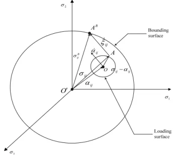
e ) and that of yield stress function (or yield surface) are decided by flow rules and hardening laws in the two-surface model. However, this time, there are two yield two-surfaces, where the kinematic yield two-surface (or loading surface) in principal stress axes resides inside the isotropic yield surface (or bounding surface) as shown in Figure 1.

Figure 1: A two-surface model in the rate-independent plasticity.

For the isotropic material, the constitutive relation in this two-surface model of plasticity is identifed as

2

ij ij kk ij

s =ld e + me ₍₄₎

in a rate-form of elastic response, where a stress point moves until it reaches the inner yield surface and strains are fully recoverable. Also, when the stress state stays on the inner yielding surface but

1



2



3



B ij



B

A

A

ij 

ij 

ij



O

O

ij 

ij ij 

resides inside the outer yielding surface (this is usually called transition region or the meta-elastic region), this rate-constitutive relation becomes

( )

3 2

1 3 ij kl kl

ij ij kk ij _p

L y

S S

H

m e

s ld e me

s

m

= +

-é ù

ê ₊ ú

ê ú ë û     (5)

Further, as the stress state becomes larger, the inner yield surface continuously approaches to the bounding surface and it finally touches the bounding surface and make this bounding surface expand. For this case, the rate-constitutive relation becomes

( )

3 2

1 3 ij kl kl

ij ij kk ij _p

B y

S S

H

m e

s ld e me

s

m

= +

-é ù

ê ₊ ú

ê ú ë û     (6)

In Eqs. (4)-(6), l is lame’s first parameter; m is shear modulus; L y

s is the inner yield stress;

B y

s is the outer yield stress; Sij is the deviatoric stress; Sij is Sij -aijrepresenting the deviatoric

stress minus the back stress;

1 2 2 n B y p B B y

H h s x

s

æ _{- ÷}ö

ç _÷

ç

= ç_ç ÷_÷

÷÷

çè ø is an isotropic hardening modulus dependent on

parameters B B B

0 1

h (=h +h s_yB), _h0B _, 1B

h , n₁, and x = x x_{ij ij}. Here, we only summarize main

formu-lation for the rate-independent two-surface plasticity model. Interested readers can refer to Banerjee et al. (1987), Chopra and Dargush (1994), and Sant (2002).

As described in Figure 1, geometrically, the kinematic hardening of the inner yield surface de-pends on a vector that joins the stress state to the bounding surface, xij. The location of A

B _is

de-termined by drawing a vector O'AABparallel to OA, B ij

s . The direction of ijis then determined to be paralled to AAB. The inner surface, which separates the elastic range and inelastic range, is composed of its center and radius expressed by the back stress (aij ) and inner yield stress (

L y

s ). Meanwhile, the outer surface, which always contains the inner yield surface, is located on the center of stress space with a radius represented by the outer yield stress ( B

y

s ). The translation of inner surface corresponds to kinematic hardening, while the expansion of outer surface produces isotropic hardening.

3 A RATE DEPENDENT TWO-SURFACE MODEL

3.1 Formulation

in p vp ij ij ij

e =e +e ₍₇₎

with in ij

e and vp ij

e representing the inelastic strain-rate and the viscoplastic strain-rate, respectively. In the past, the above approach had been proven to be effective when accounting for the hyste-resis loop with the rounded corners in stress-transition from elastic to inelastic or vice versa [Brad-ley and Yuen (1983 ); Tirpitz and Schwesig (1992); Lubliner (2008)]. In addition, as in the existing two-surface plasticity model, a present two-surface viscoplasticity model utilizes the following yield functions such as

3 : 2

y y

L L

L e ij ij

g =s -s = S S -s (8)

and

3 : 2

y y

B B

B e ij ij

g =s -s = S S -s (9)

depending on kinematic hardening and isotropic hardening rules. Here, s_e is the von Mises effec-tive stress and the symbol “:” designates the product contracted twice. Thus, three separate regions in Figure 1 are identified with these yield functions: g_L < 0 (elasticity); g_L > 0 and g_B < 0

(meta-elasticity); g_B > 0 (both kinematic and isotropic hardening rules are effective). Once the

stress-state is identified with these criteria, each portion of the inelastic strain is given by flow rule and nomality hypothesis:

p I

ij

g

e l

s ¶ =

¶ 

 where I B or L ₍₁₀₎

vp I

ij

g p

e

s ¶ =

¶

  where I =B or L ₍₁₁₎

In Eq. (10), the magnitude of the plastic strain increment l can be decided by the consistency condition g_I =g_I = 0. Otherwise, the magnitude of the viscoplastic strain increment p is

deter-mined from a potential j

( , , B)

ij ij y

p =j s a s ₍₁₂₎

that is the function of the stress s_ij, the back stress a_ij, and the magnitude of bounding surface

B y

s .

With adoption of the hyperbolic sine function for j (Dunne and Petrinic, 2005), p can be

2

2 3

sinh ( ) sinh :

2

n n

B L B L

e y y ij ij y y

p =Cé_ëê B s -s -s _úù_û =Céê_ê Bçæç_ç S S -s -s _÷÷÷öù_úú

÷÷ çè ø ê ú ë û    (13)

In Eq. (13), C and B represent material parameters associated with viscosity. Also,

n

represents the deviatoric stress that can be either S_ij or S_ij.

Thus, the viscoplastic strain rate is identified as

3 2 ij vp ij e S p e s = 

  where S_ij = S_ij or S_ij (14)

and consequently, the inelastic strain is given by

3 2

e I e I

ijmn pqkl kl

mn pq ij

in I I

e

ij ij I I I I e

mnpq

mn pq pq pq

g g

C C

S

g g

p p

g g g g

C

e

s s

e l

s s s

s s e s

¶ ¶ ¶ ¶ ¶ ¶ = + = + ¶ ¶ ¶ ¶ ¶ ¶ -¶ ¶ ¶ ¶  _ 

   ₍₁₅₎

Overall, in the present two-surface viscoplasticity model, the consitutive relation of isotropic material results in

2

ij ij kk ij

s = ld e + me ₍₁₆₎

( )

3

2 3

1 3

ij kl kl ij

ij ij kk ij _p

e L

y

S S S

p H

m e

s ld e me m

s s

m

= + - _{é ù}

-ê ₊ ú

ê ú ë û      (17)

( )

3

2 3

1 3

ij kl kl ij

ij ij kk ij _p

e B

y

S S S

p H

m e

s ld e me m

s s

m

= + -

-é ù

ê ₊ ú

ê ú ë û      (18)

for the elastic response, kinematic hardening response, and both kinematic and isotropic hardening response, respectively.

3.2 Finite Element Implementation

1 ₂ 1

n n n

ij ij ij

S + =S + mDe + ₍₁₉₎

1 1 1 1

3

n n n

ij Sij ij kk

s + ₌ + ₊ d s + ₍₂₀₎

1 3

n n n

ij Sij ij kk

s = + d s (21)

1 3

n n n

ij ij ij kk

e =e - d e (22)

where eij is deviatoric strain tensor, and n and n+1 represent time-steps.

Subtracting Eq.(21) from Eq.(20) with the strain decomposition, and the relationship between strain and deviatoric strain in Eq.(22), one finds

1 1 1 1

2

3 3 3 3

p vp

p vp

ij ij ij kk ij ij kk ij ij kk ij kk

s mæç e d e e d e e d e ö÷ d s

D = ç_çD - D - D + D - D + D ÷ +_÷÷ D

è ø (23)

Using a plastic flow rule and viscoplastic flow rule, Eq.(23) yields

1 1 1 1

2

3 3 3 3

ij ij ij kk ij ij ij kk

g g g g

p p

s m e d e l d l d d s

s s s s

æ _{¶ ¶ ¶ ¶ ÷}ö

ç

D = ç_çD - D - + - + ÷ +_÷÷ D

è ¶ ¶ ¶ ¶ ø (24)

Finally, one can obtain the following incremental formulation.

( )

2 3

1 3

ij kl kl ij

ij ij ij kk _p

e y

S S S

p H

m e

s m e ld e m

s s

m

D

D = D + D - - D

æ _ö÷

ç _{+ ÷}

ç _÷

ç _÷

çè ø

(25)

Eq. (25) is numerically into the commercial finite element code, ABAQUS, where a certain iter-ation scheme is introduced to solve nonlinear equiter-ations at the element and global system level (Bathe and Cimento (1980)). The following is a brief explanation about how the nonlinear solver works (here, subscript indices are omitted to avoid complexity). First, all the variables are initial-ized with corresponding time-step. Then, the solution (t_{U , nodal displacements) and other internal}

variables such as strain (t_{e) and stress (}t_{s) are stored at time (t), where the iteration counter (i) is}

fixed as 1. Variables at the time-step of (t+t) are calculated and updated through iterations with convergence criteria and/or a maximum number of iterations.

For example, the stress is updated from a known converged solution as

1 t t 1

t t i t t t i

t C d

s s +D e

+D - _{= +}

_ò

At the element level, the tangent constitutive matrix (t+Dt_Ci-1_{) is updated with a certain}

itera-tive scheme, and consequently, the global stiffness matrix (t+Dt_Ki-1_{) and nodal force vector}

(t+Dt_Fi-1_{) corresponding to the interanl element stresses (}t+Dt_si-1_{) are computed by using a}

1 1

e

t t i T t t i

V e

K B C BdV

+D - ₌

_{å ò}

-(27)

1 1

e

t t i T t t i

V e

F B s dV

+D - ₌

_{å ò}

-(28)

At the global system level, the solution is obtained in terms of the incremental nodal displace-ments (_DUi_{) by solving the following set of equations}

1 1

t+Dt_K i- _DUi ₌ t+Dt_R-t+Dt_Fi

-(29)

with t+Dt_{R representing the externally applied nodal force vector to the time-step, t+}

t

 . In solv-ing the global solution of incremental displacement i-1_DUi_{, interative scheme is also utilized to}

update t+Dt_Ki-1 _{along with convergence criteria and/or a maximum number of iterations. Finally,}

the numerical solution of displacements at the time-step (t+t) is updated by

1

t+Dt_Ui ₌ t+Dt_Ui- _{+ DU}i ₍₃₀₎

and strains are calculated from these updated displacements.

In the present work, we adopt the Cash-Karp method (one of embedded Runge-Kutta methods) as the iterative method for updating t+Dt_Ci-1_{, while the Newton-Raphson iterative method is used}

to solve the global system equation with updating t+Dt_Ki-1_.

4 NUMERICAL EXAMPLES

In this section, we verify the present two-surface model for viscoplasticity with representative ex-amples including both monotonic and cyclic loading cases, where both experimental results by Chang (1985) and numerical simulation results by the kinematic hardening model are provided for the reference.

4.1 Experimental Results

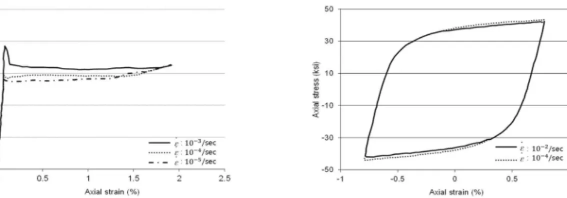
For the monotonic loading case, Chang experimentally tests A36 structural steel with three differ-ent strain rates of 10-3/sec, 10-4/sec, and 10-5/sec, in each of which loading was increased until 2% axial strain was achieved. Also, in cyclic tests, there are four different types of loading as shown in Figure 2, where all the specimen were loaded in the axial direction and the loading continued until it was stabilized. In particular, for the case 1 and the case 2, the loading was increased until 0.8% axial strain was attained, while the loading was increased until 0.6%, 1.2%, and 1.5% axial strain were obtained for the case 3 and the case 4.

(a) Strain rate of 10-4_{/sec (Loading Type 1) (b) Strain rate of 10}-2_{/sec (Loading Type 2)}

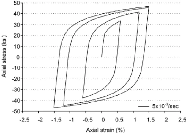
(c) strain rate of 10-4_{/sec (Loading Type 3) (d) strain rate of 5 x 10}-3_{/sec (Loading Type 4)}

Figure 2: Cyclic loading cases.

As shown in Figure 3, three different values of maximum were observed in the monotonic test: 32.5 ksi after initial peak (strain rate 10-3/sec); 30ksi (strain rate: 10-4/sec); 28.5 ksi (strain rate: 10

-5_{/sec).This indicates that the faster strain rate gives the higher stress after yielding. Also, it is}

ob-served that the higher strain rate gives the longer plastic plateau and strain hardening effects are negligible in these monotonic tests. With reference to the strain rate of 10-5/sec, the yield stress at a strain rate of 10-4/sec was increased by 5%, and the yield stress at strain rate of 10-3/sec was in-creased by 14%.

Figure 3: Experimental results under monotonic loading. Figure 4: Experimental results under loading type 1 & 2.

Figure 5: Experimental result under loading type 3. Figure 6: Experimental result under loading type 4.

4.2 Numerical Simulation Results

With a user subroutine (UMAT) in the ABAQUS, both rate-dependent nonlinear kinematic hard-ening model two-surface models are implemented by the authors. For fair comparison between these two models, we employ one four-node bilinear axisymmetric element (CAX4) for the cylinder-type specimen in every numerical simulation examples, as shown in Figure 7. Also, in numerical simula-tion, Newton-Raphson method is adopted with fixing the maximum number of iteration as 1000 and incremental displacement as 10-9 under such conditions, we checked that all the numerical solu-tions satisfy convergence criteria of residual force (less than 10-5) and displacement (less than 10-8), respectively.

(a) Geometry of specimen (b) Finite element (CAX4)

4.2.1 Nonlinear Kinematic Hardening Model

The main difference between the developed two-surface model and the nonlinear kinematic harden-ing model [Chaboche, 2008] for the rate-dependent plasticity is that von Mises yield surface cannot expand in the nonlinear kinematic hardening model, while the developed two-surface model allows both expansion and translation of von Mises yield surface. In addition, in the developed two-surface model, we differentiate inelastic strain as the rate-dependent ( vp

ij

e ) and the rate-independent part ( p

ij

e ) as in Eq. (7). Thus, we have the following equations for the nonlinear kinematic hardening model

3 2

ij vp

ij

ij e

S g

p p

e

s s

¶

= =

¶

   ₍₃₁₎

( vp) 3 ij

e e

ij ijkl kl kl ijkl kl

e S

C C p

s e e e m

s

æ _ö÷

ç _÷

ç

= - = _ç - _÷÷

ç ÷

çè ø

  

  (32)

whereas the developed two-surface model has Eqs. (15)-(18).

In numerical simulation of the nonlinear kinematic hardening model, we take material proper-ties and parameters as shown in Table 1.

Young's modulus(E): 28,500 ksi(196,500 MPa), Poisson's ratio () : 0.35 Yield stress(y): 30 ksi (206.84 MPa)

Material parameters of the hyperbolic sine function: C= 1.E+2; B= 1.E-8; n2 = 5.0

Table 1: Material properties and model parameters employed in the kinematic hardening model.

As shown in Table 1, the yielding stress is specified as 30 ksi (206.84 MPa) for A36 steel, and this value is adopted in numerical simulation with calibration of experimental results from Chang (1985).

Figure 8: Numerical results under monotonic loading (nonlinear kinematic hardening model).

Figure 9: Numerical results under cyclic loadings of type 1 and type 2 (nonlinear kinematic hardening model).

Figure 10: Numerical result under cyclic loadings of type 3 (nonlinearkinematic hardening model).

Axi

al

st

re

ss

(k

si

)

-50 -40 -30 -20 -10 0 10 20 30 40 50

-2.5 -2 -1.5 -1 -0.5 0 0.5 1 1.5 2 2.5 Axial strain (%)

Figure 11: Numerical result under cyclic loadings of type 4 (nonlinearkinematic hardening model).

4.2.2 Two-Surface Model

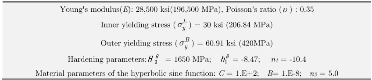
For numerical simulation of the two-surface model, basically, the same parameters in Table 1 are utilized. Additional parameters adopted in numerical simulation to account for combined effects of both kinematic nd isotropic hardening are summarized in Table 2. In particular, both inner yielding stress and outer yielding stress are introduced here instead of a single yielding stress. Again, every parameter in Table 2 is calibrated from experimental results by Chang (1985), here.

Young's modulus(E): 28,500 ksi(196,500 MPa), Poisson's ratio () : 0.35

Inner yielding stress (s_yL) = 30 ksi (206.84 MPa) Outer yielding stress (s_yB) = 60.91 ksi (420MPa) Hardening parameters: B

H

0 = 1650 MPa;

B h

1 = -8.47; n1 = -10.4

Material parameters of the hyperbolic sine function: C = 1.E+2; B= 1.E-8; n2 = 5.0

Table 2: Additional material properties and model parameters adopted in the two-surface model.

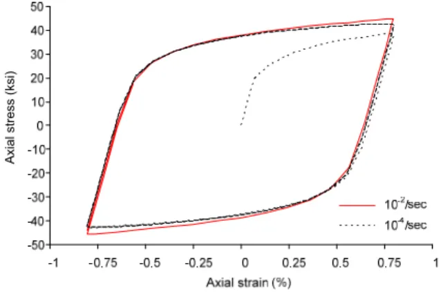
closer to experimental results, compared to those from the nonlinear kinematic hardening model. Also, for all the cases, the two-surface model gives reasonably good rounded shape of hysteresis as detected in experiments.

Figure 12: Numerical results under monotonic loading (two-surface model).

Figure 13: Numerical results under cyclic loadings of type 1 and type 2 (two-surface model).

Figure 14: Numerical result under cyclic loadings of type 3 (two-surface model).

Ax

ia

l st

re

ss

(ks

Figure 15: Numerical result under cyclic loadings of type 4 (two-surface model).

5 CONCLUSIONS

In this paper, we develop a two-surface model for rate-dependent plasticity as an extension of the two-surface model in the rate-independent plasticity by Banerjee et al. (1987). The model combines both isotropic and kinematic hardening rules, where the constitutive relation is modified to account for rate-effects. In particular, this model has three separate regions with two bounding surfaces. Thus, when the stress remains in the lower bound, the response is elastic. Also, when stress exceeds the upper bound, the response shows both kinematic and isotropic hardening. In the middle range where the stress resides beteween the lower bound and the upper bound, the response only follows the kinematic hardening rule. With use of a subroutine UMAT, the present model is implemted in the commercial finite element software, ABAQUS. Then, this model is validated through both monotic and cycling loading cases with comparison to experiments and the nonlinear kinematic hardening model. The present model shows excellent agreement with experiments in both maximum stress and shape of hysteresis, while the nonlinear kinematic hardening model is not suitable to account for the shape of hysteresis.

Acknowledgements

This work was supported by the Dong-A University research fund.

References

Abdel-Karim, M.and Ohno, N. (2000). Kinematic hardening model suitable for ratchetting with steady-state. Inter-national Journal of Plasticity, 16: 225-240.

Armstrong, P.J. and Frederick, C.O. (1966). A mathematical presentation of the multiaxial Bauschinger effect. CEGB Report RD/B/N731. Berkeley Nuclear Laboratories, Berkeley, UK.

Banerjee, P.K., Wilson, R.B., and Raveendra, S.T. (1987). Advanced applications of BEM to three dimensional problems of monotonic and cyclic plasticity. International Journal of Mechanical Science, 29(9): 637–653.

Bari, S. and Hassan, T. (2000). Anatomy of coupled constitutive models for ratcheting simulation. International Journal of Plasticity, 16: 381–409

-50 -40 -30 -20 -10 0 10 20 30 40 50

-2.5 -2 -1.5 -1 -0.5 0 0.5 1 1.5 2 2.5 Axial strain (%)

Bari, S. and Hassan, T. (2002). An advancement in cyclic plasticity modeling for multiaxial ratchetting simulation. International Journal of Plasticity, 18: 873-894.

Bathe, K. J. and Cimento, A. P. (1980) Some practical procedures for the solution of nonlinear finite element equa-tions. Computer Methods in Applied Mechanics and Engineering, 22: 59-85

Bodner, S.R. and Partom, Y. (1972). A large deformation elastic-viscoplastic analysis of a thick-walled spherical shell. Journal of Applied Mechanics, ASME, 39: 751-757.

Bradley, W.L. and Yuen, S. (1983). A new uncoupled viscoplastic constitutive model. NASA, Lewis Research Center Nonlinear Constitutive Relations for High Temperature Application; 217-234

Chaboche, J.L. (1977). Viscoplastic Constitutive Equations for the Description of Cyclic and Anisotropic Behavior of Metals, Bulletin of Polish Academy of Sciences Technical Sciences, 25: 33-42.

Chaboche. J.L. (1986). Time independent constitutive theories for cyclic plasticity. International Journal of Plasticity, 2: 149-188.

Chaboche. J.L. (1989). Constitutive equations for cyclic plasticity and cyclic viscoplasticity, International Journal of Plasticity, 5: 247-302.

Chaboche. J.L. (1991). On some modifications of kinematic hardening to improve the description of ratcheting effects. International Journal of Plasticity, 7(7): 661–678.

Chaboche. J.L. (2008). A review of some plasticity and viscoplasticity constitutive theories, International Journal of Plasticity, 24: 1642-1693.

Chaboche. J.L., Rousselier. (1983). On the Plastic and Viscoplastic Constitutive Equations-Part II: Application of Internal Variable Concepts to the 316 Stainless Steel. Journal of Pressure Vessel Technology, 105(2): 159-164. Chang, K.C. (1985). Behaviour of structural steel under cyclic and nonproportional loading. Ph.D dissertation, The State University of New York at Buffalo, USA

Chopra, M.B. and Dargush, G.F. (1994). Development of bem for thermoplasticity. International Journal of Solids and Structures, 31(12/13): 1635-1656

Dafalias, Y.F., Popov, E.P. (1975). A model of nonlinearity hardening materials for complex loading. Acta Mechani-ca, 21(3): 173–192.

Dargush, G.F. and Soong, T.T. (1995). Behavior of metallic plate dampers in seismic passive energy dissipation systems. Earthquake Spectra, 11(4): 545–568.

Dune, F. and Petrinic, N. (2005) Introduction to computational plasticity, Oxford university press. Hibbit, Karlsson and Sorensen, Inc. (2008). Abaqus user's guide, v. 6.8. HKS Inc. Pawtucket, RI, USA.

Kalali, A.T, Moud, S.H, and Hassani, B. (2016) Elasto-plastic stress analysis in rotating disks and pressure vessels made of functionally graded materials. Latin American Journal of Solids and Structures, 13(5): 819-834

Kang, G.Z. (2004). A viscoplastic constitutive model for ratchetting of cyclically stable materials and its finite ele-ment impleele-mentation. Mechanics of Materials, 36:299-312

Kang, G.Z., Gao, Q., and Yang, X.J. (2004). Uniaxial and multiaxial ratchetting of SS304 stainless steel at room temperature: experiments and visco-plastic constitutive model. International Journal of Nonlinear Mechanics, 39: 843-857.

Kang, G.Z., Gao, Q., Cai, L.X., Yang, X.J. Sun, Y.F. (2002). Experimental study on the uniaxial and nonpropor-tionally multiaxial ratchetting of SS304 stainless steel at room and high temperatures. Nuclear Engineering and Design, 216: 13-26.

Krieg, R.D. (1975). A practical two surface plasticity theory. Journal of Applied Mechanics, ASME, 42(3): 641–646. Lubliner, Jacob (2008). Plasticity Theory (Revised Edition). Dover Publications.

McDowell, D.L. (1992). A Nonliear Kinematic Hardening Theory for Cyclic Thermoplasticity and Thermoviscoplas-ticity. International Journal of Plasticity, 8 : 695-728.

McDowell, D.L., (1995). Stress state dependence of cyclic ratchetting behavior of two rail steels. International Jour-nal of Plasticity, 11(4): 397–421.

Mroz, Z., (1967). On the description of anisotropic work hardening. Journal of Mechanics Physics of Solids, 15(3): 163–175.

Ohno, N. and Wang, J.D., (1993a). Kinematic hardening rules with critical state for activation of dynamic recovery, part I, formulation and basic features for ratchetting behavior. International Journal of Plasticity, 9(3): 375–390. Ohno, N. and Wang, J.D., (1993b). Kinematic hardening rules with critical state for activation of dynamic recovery, part II, application to experiments of ratchetting behavior. International Journal of Plasticity, 9(3): 391–403.

Prager, W. (1956). A new method of analyzing stresses and strains in work hardening plastic solids. Journal of Ap-plied Mechanics, 23: 493-496.

Sant, R.S. (2002). Evolutionary structural optimization for aseismic design. Ph.D dissertation, The State University of New York at Buffalo, USA

Tanaka, E. (1994). A non-proportionality Parameter and a Viscoplastic Constitutive Model Taking into Amplitude Dependencies and Memory Effects of Isotropic Hardening, European Journal of Mechanics A/Solids, 13: 155-173. Tanaka, E., and Yamada, H. (1993). Cyclic creep, mechanical ratchetting and amplitude history dependence of modified 9Cr–1Mo steel and evaluation of unified constitutive models. Transactions of the Japan Sciety of Mechani-cal Engineers, 59: 2837–2843.

Tirpitz, E.R. and Schwesig M. (1992) A unified model approach combining rate dependent and rate independent plasticity, Low Cycle Fatigue and Elasto-Plastic Behaviour of Materials, 3: 411-417.

Tsai, K.C., Chen, H.W., Hong, C.P., Su, Y.F. (1993). Design of steel triangular plate energy absorbers for seismic resistant construction. Earthquake Spectra, 9(3): 505–528.

Yaguchi, M., Takahashi, Y., (2000). A viscoplastic constitutive model incorporating dynamic strain aging effect during cyclic deformation conditions. International Journal of Plasticity, 16: 241–262.