Multiple quality tests for analysing CO<sub>2</sub> fluxes in a beech temperate forest

(1)

BGD

4, 4197–4228, 2007

Quality tests for analysing CO₂ fluxes

B. Longdoz et al.

Title Page

Abstract Introduction

Conclusions References

Tables Figures

◭ ◮

Back Close

Full Screen / Esc

Printer-friendly Version

Interactive Discussion

EGU

Biogeosciences Discuss., 4, 4197–4228, 2007 www.biogeosciences-discuss.net/4/4197/2007/ © Author(s) 2007. This work is licensed

under a Creative Commons License.

Biogeosciences Discussions

Biogeosciences Discussionsis the access reviewed discussion forum ofBiogeosciences

Multiple quality tests for analysing CO

₂

fluxes in a beech temperate forest

B. Longdoz, P. Gross, and A. Granier

INRA, UMR1137 Ecologie et Ecophysiologie Foresti `ere, Centre de Nancy, 54280 Champenoux, France

Received: 30 August 2007 – Accepted: 18 October 2007 – Published: 13 November 2007

(2)

BGD

4, 4197–4228, 2007

B. Longdoz et al.

Title Page

Tables Figures

◭ ◮

Back Close

Full Screen / Esc

EGU

Abstract

The eddy covariance (EC) measurements are widely used to estimate the amount of carbon sequestrated by terrestrial biomes. The data quality and the selection of the correct EC records become an important step in the CO₂ flux determination proce-dure. In this paper an innovative combination of existing assessment tests is used to 5

give a relatively complete evaluation of the net ecosystem exchange measurements. For the 2005 full-leaf season at the Hesse site, the percentage of bad quality data is relatively high (59.6%) especially during night-time (68.9%). This result strengthens the importance of the data gap filling method. The filtering used does not lead to a real improvement of the accuracy of the relationship between the CO₂fluxes and the 10

climatic factors. The soil respiration spatial heterogeneity (on a site with relatively ho-mogenous vegetation pattern) seems to be too important to allow this improvement. However, the data rejected present some common characteristics. Their removal lead to a 10% increase in the total amount of CO₂ respired and photosynthesised during the 2005 full-leaf season. Consequently the application of our combination of multiple 15

quality tests is able improve the inter-annual analysis. The question of a systematic application on the large database like the CarboEurope and FLUXNET is legitimate.

1 Introduction

Carbon dioxide exchanges between the terrestrial ecosystems and the atmosphere are of major importance for climate change and therefore for the future of the vegetation 20

(Houghton et al., 1998). The quantification of CO2fluxes at the ecosystem-atmosphere interface is one of the primordial steps to improve our knowledge about the ecosystem carbon budget. The eddy covariance (EC) technique (Aubinet et al., 2000) provides the opportunity to have a direct measurement of these fluxes. Sites equipped with EC systems spread around the world (Baldocchi et al., 2001) with, at the present time, 25

(3)

BGD

4, 4197–4228, 2007

B. Longdoz et al.

Title Page

Tables Figures

◭ ◮

Back Close

Full Screen / Esc

EGU

been running continuously for more than 10 years. The EC technique is based on high frequency (10–20 Hz) records of wind speed components, CO2and H2O concen-trations. The amount of data produced is so large that the detection of instrumental anomalies becomes very difficult. Moreover, the flux determination includes several methodological choices (Finnigan et al., 2003) and requires selection of periods with 5

adequate micro-meteorological conditions (Feigenwinter et al., 2004; Rebmann et al., 2005). All these difficulties lead to errors and propagation of uncertainties that are able to mask some properties of biophysical processes. The improvement of the EC dataset quality has become a real challenge for the EC scientific community (Richardson et al., 2006a; Papale et al., 2006).

10

One of the problems met with the EC measurements are the short-term net CO₂flux fluctuations during night-time (Longdoz et al., 2004) without any biophysical explana-tion. Two reasons have already been identified. The CO2produced by the respiration of the ecosystem components can be stored in the canopy air or blown horizontally by advection (Paw et al., 2000). This CO2 is not registered by the EC system. For 15

our temperate beech forest site (Hesse, France), corrections with canopy air storage measurement and selection of the data without advection (Aubinet et al., 2005) have not completely erased this problem. Consequently, the question of the quality of the data generated by the EC systems arises

Di_fferent authors have presented several quality tests for the selection of the EC 20

data (Vickers and Mahrt, 1997; Foken and Wichura, 1996; G ¨ockede et al., 2004) and several methods to fill the gaps produced by this data selection (Falge et al., 2001; Hui et al., 2004; Ruppert et al., 2006). In this study, we combine most of the tests proposed for the CO2 flux. This innovative grouping is applied to the records from the Hesse site for the full-leaf 2005 season. This period presents some reasonably 25

(4)

BGD

4, 4197–4228, 2007

B. Longdoz et al.

Title Page

Tables Figures

◭ ◮

Back Close

Full Screen / Esc

EGU

quality tests is evaluated by comparison with the datasets including or not including the records incriminated by the tests. The analysis is performed on the relationships between CO2fluxes and climatic factors and on the total fluxes accumulated during the full-leaf 2005 season.

2 Material and methods 5

2.1 Site

All the data used in the present analyses come from an experimental plot located in the state forest of Hesse (48◦₄₀′_{N, 7}◦₀₄′_{E, North-east of France). This site belongs to}

the CarboEurope network. The climate is temperate with 950 mm and 10.1◦_{C for mean}

annual rainfall and air temperature. The stand is composed mainly (90%) of Beech 10

(Fagus sylvatica). For the period considered in this paper (full-leaf season from 15 May to 14 October 2005) the trees were 39 years old and 17 m high (mean value), the LAI (5.1 m2m−2_{) and tree density (2916 stem/ha) were relatively low compared to the}

previous years (mean LAI 7.3 m2m−2_{) because of the thinning performed during the}

winter 2004–2005. The roughness length was 0.4 m. The gentle slope (approximately 15

3% going down in the Northeast direction) is sufficient to induce advection during the stable nights (Aubinet et al., 2005). The distance between the EC tower and the for-est edge varies from 390 m to 1610 m. The full-leaf season selected (2005) can be qualified as relatively normal when compared to the mean climate of the eight previous years . The mean air temperature is equal (16◦_{C), the total amount of precipitation is} 20

slightly lower (381–416 mm) and the cumulative global radiation slightly higher (2957– 2873 MJ m−2_{) for 2005. A more detailed description of the site can be found in Granier}

(5)

BGD

4, 4197–4228, 2007

B. Longdoz et al.

Title Page

Tables Figures

◭ ◮

Back Close

Full Screen / Esc

EGU

2.2 Fluxes measurements

The net CO2fluxes between the ecosystem and the atmosphere (Fc) were measured with an eddy covariance system composed by a sonic anemometer Solent R3 (Gill In-struments Ltd, Lymington, UK) and an infrared gas analyser Li-Cor 6262 (Li-Cor Inc., Lincoln, NE, USA). The anemometer measuring the three components of the wind ve-5

locity and sonic temperature (u,v,w,T) at 20 Hz is located on a tower at 23.5 m above ground. The IRGA measuring CO₂ and H₂O concentrations at 10 Hz is located at the ground level, analysing the air sucked from a sampling point close to the anemometer with an air flow rate of 6 l min−1_{. A mass flow controller (Model 5850, Brooks,}

Vee-nendaal, Netherlands) controls the airflow. The computer acquires the data with the 10

software Eddymeas (Kolle and Rebmann, 2007). To improveu,v andw data, correc-tion for sonic anemometer angle of attack errors is performed (Naka¨ıet al., 2006). This error becomes significant when the wind vector angle to the horizontal plane is supe-rior to 20◦ _{(threshold value depending on the sonic anemometer type). It is provoked}

by transducers self-sheltering or flow distortion induced by the anemometer frame. For 15

each half-hour, the Fc fluxes are calculated from high frequency u, v, w and CO₂ concentration measurements using block averaging operator (Finnigan et al., 2003) and planar fit as coordinates rotation method (Wilczak et al., 2001). Finally, frequency correction applied toFc follows the procedure proposed by Aubinet et al. (2000).

The net ecosystem exchange (NEE) is obtained by the summation of Fc and CO2 20

storage in the canopy air (Sc). Sc corresponds to the difference between the total amount of CO₂below the eddy covariance measurement height, at the beginning and the end of the half-hour. This amount of CO₂is estimated from a profile of concentration estimated from measurements at 6 different heights (22 m, 10.4 m, 5.2 m, 2 m, 0.7 m, 0.2 m). These measurements are performed with an infrared gas analyser Li-Cor 6262 25

(6)

BGD

4, 4197–4228, 2007

B. Longdoz et al.

Title Page

Tables Figures

◭ ◮

Back Close

Full Screen / Esc

EGU

2.3 Quality control procedures

The eddy covariance data treatment used in this study includes several tests to con-trol the data quality and detect flux sampling problems. First, following Vickers and Mahrt (1997), the records are flagged to identify abnormalities that may result from instrumental or data recording problems coming from the anemometer or the IRGA 5

(corresponding to hard flag in Vickers and Mahrt). The tests check in the high fre-quency measurements of wind velocity and CO2concentration the presence of spikes, discontinuities of mean or variance, unrealistic data, large higher-moment statistics (skewness and kurtosis) or standard deviation value out of tolerable range. The half-hoursFc are flagged when parameters reflecting the importance of these presences 10

exceed threshold values. As proposed by Vickers and Mahrt (1997), the thresholds are empirically adjusted for the Hesse site by inspection of frequency distributions of the parameters. The objective is to flag any records with obvious instrument problems. This threshold determination procedure realised for the Hesse 2005 full-leaf season can be illustrated by the choice of upper limit of the acceptable range for the kurtosis 15

of CO₂ concentration data , which is the more selective test (see results section). The upper limit of the kurtosis is set to 7.9 to be sure to flag the half-hour record like the one presented in the Fig. 1a. Indeed, the kurtosis of this half-hour is 8.1 because of few irregularities (too large to be considered as spikes) that happen at regular interval indi-cating their instrumental origins. This half hour record has to be flagged. Moreover, we 20

have not found a half-hour with a lower kurtosis and presenting apparent instrumental problem. For example, important intermittent turbulent events (Fig. 1b) can explain a kurtosis slightly lower than the threshold (7.7) and should not be flagged. Contrary to Vickers and Mahrt (1997) all the half-hours flagged have not been individually analysed to verify the origin of the flux-sampling problem. This procedure is not materially feasi-25

(7)

BGD

4, 4197–4228, 2007

B. Longdoz et al.

Title Page

Tables Figures

◭ ◮

Back Close

Full Screen / Esc

EGU

The last test to detect instrumental abnormalities is the verification of the airflow rate in the tubing transporting the air from the sampling point (at the top of the tower) to the EC IRGA. This rate is controlled and measured by a mass flow controller (Tylan 261, Tylan Corporation, Torrance, CA, USA). It is set to 6 l min−1_{leading to a constant time}

lag of 4.8 s betweenw and C measurement. The flag is activated when the airflow 5

rate is 10% below or above the desired value. This range is chosen because the post-processing programme is able to correct any deviation of the time lag in this range.

The other quality assessment tests do not refer to instrumental abnormalities but verify the stationarity forFc and the inclusion of the Fc footprint area in the targeted ecosystem. The stationarity test procedure follows the method presented by Foken 10

and Wichura (1996). TheFc value determined for the half-hour period is compared to the mean out of six 5-min Fc from the same period. The flag is activated when the difference between both values (due for example to changing weather conditions) is above 30% so when theFc data could not be used for fundamental research (Foken et al., 2004). For the footprint test, the Schuepp model (Schuepp et al., 1990) modified 15

by Soegaard et al. (2003) determines the Fc footprint area. The record is flagged when more than 10% ofFc is coming from a patch (25 m long, 5◦ _{large) located out}

of Hesse beech forest. The forest edge is determined with the Hesse land use map already utilized in Rebmann et al. (2005).

2.4 Datasets 20

Two datasets are established both compiling the main micrometeorological variables (global radiation, air and soil temperature, photosynthetic photon flux density, soil water content, air humidity, friction velocity. . . ) and the NEE values for the 7344 half-hours between the 15 May and 14 October 2005. At the beginning of the analysis, in one of the datasets, the gaps in the NEE correspond only to the breakdown and maintenance 25

(8)

BGD

4, 4197–4228, 2007

B. Longdoz et al.

Title Page

Tables Figures

◭ ◮

Back Close

Full Screen / Esc

EGU

different dataset partitioning are applied during the analysis. The partitioning between night and day is based on the global radiation (Rg) with night records corresponding toRg below 3 W m−2_{. During night-time NEE corresponds to ecosystem respiration}

(Reco) and during daytime to the sum of gross primary productivity (GPP) plus Reco. The second division aims at isolating the periods without soil water stress forReco. As 5

soil respiration represents usually the major part ofReco (Law et al., 1999; Longdoz et al., 2000) and because Ngao (2005) has demonstrated that soil respiration in the Hesse forest is limited by water depletion when soil water content on the first 10 cm (SWC) is below 0.2 m3m−3_{; we have adopted this threshold for the dataset repartitioning.}

Different authors (Staebler et al., 2004; Aubinet et al., 2005) have shown that NEE 10

estimated by summation ofFc andSc can underestimate CO₂exchanges during pe-riods with low turbulence (low friction velocity u*). Night-time Reco measurements clearly highlight this underestimation. At constant temperature,Reco drops down when

u* decreases. This observation has no apparent biophysical explanation. At the Hesse site, additional measurements have proven that some CO2emitted during night by the 15

ecosystem components goes out of the forest by horizontal advection when air mixing is limited (Aubinet et al., 2005). This CO₂ is not detected by the eddy covariance or profile concentration measurement systems explaining flux underestimation. We have established au* threshold below whichReco is not correctly measured by a two steps procedure. In the first step, the temporal variability ofReco, mainly due to temperature 20

fluctuations, is determined. Using data during periods without water stressed, theReco dependence on temperature is fitted (regression algorithm presented in the following section) using aQ₁₀relationship (Black et al., 1996):

Reco₌Reco_Tref·Q( T−Tref

10 )

10 (1)

whereQ10 is the parameter reflecting the temperature sensibility and RecoTref is the 25

Reco value for a reference temperature (Tref). Each half-hour Reco is then divided

byQ( T−Tref

10 )

10 to obtain a valueRecos that should be relatively constant during non water

(9)

BGD

4, 4197–4228, 2007

B. Longdoz et al.

Title Page

Tables Figures

◭ ◮

Back Close

Full Screen / Esc

EGU

each class, we compute theReco_s class average (Reco_s)_cl, and theReco_s averaged on all the data withu* above the upper limit of the class (Recos)hi. The objective is

to detect the classes with a (Recos)cl significantly lower than (Recos)hi (comparison

procedure described in the following section). Among these last classes, the one with the higher u* is selected. The u* threshold corresponds then to the upper limit of 5

this class. Because theQ10 relationship fit depend on the available dataset, the u* threshold determination procedure is applied separately on DSEFR and DSIFR.

2.5 Statistical analysis and regression

All the statistical analysis and non-linear regressions are performed by Statgraphics Plus software (Statistical Graphics Corp., Herndon, VA, USA). The two data sample 10

comparisons are designed to determine whether they are significantly different by run-ning a t-test to compare the means of the two samples. The equality of the variances of the two samples is assumed. ANOVA (F-test) is used for the multi-groups comparison. The non-linear regression algorithm is an iterative procedure, determining the param-eters that minimize the residual sum of squares (Marquardt method). The non-linear 15

regressions are used to determine the relationship between meteorological variables and fluxes. For some of the regressions with a single independent variable, it is suitable to reduce the possible impacts of spatial heterogeneity and other variables. Then the regressions are performed with bin-average fluxes where the averages are performed for independent variable classes. The average are weighted with weights proportional 20

(10)

BGD

4, 4197–4228, 2007

B. Longdoz et al.

Title Page

Tables Figures

◭ ◮

Back Close

Full Screen / Esc

EGU

3 Results – discussion

3.1 Quality control results

Among the 7344 half-hours treated, only 2.1% corresponds to total breakdown (mainly electricity failure) or maintenance of the EC system and 2.6% to specific maintenance or bad functioning of the profile sampling system. On the remaining Fc data (7190 5

values), flags are activated on 48.8% of the data (3508 half-hours) consequently on 47.8% of the total period. This is a relatively high percentage but not very surprising compared to the proportion already presented in the literature. Rebmann et al. (2005) flagged 28% of the HesseFcfor the summer 2000 only with the stationarity test. Vick-ers and Mahrt (1997) flagged during their measurement campaigns one-third of the 10

records with the Haar variance criteria and one-half for too large kurtosis.

In our procedure, the causes of the Fc flags could be divided in five categories: anemometer, CO2 IRGA and mass flow controller malfunctioning, lack of stationarity and too large footprint. The percentages of Fc flags due to each category are pre-sented in the Table 1. Two tests appear to be highly restrictive: the stationarity and 15

the CO2 IRGA anomalies. The stationarity flag percentage is close to that estimated by Rebmann et al. (2005) for the Hesse summer 2000 (28%). To go one-step further in the analysis and according to the Sect. 2.3, we subdivided the CO₂flag into seven tests: spikes, mean discontinuity, variance discontinuity, absolute limits, skewness, kurtosis and standard deviation. The kurtosis is more selective (Table 2) with flags on 20

31.9% of the total period (32.6% of non-affectedFc). This predominance of the kurto-sis test on the other ones has been also observed by Vickers and Mahrt (1997) on their own measurements. The sum of all the half-hours flagged by the different CO2 tests (3960) exceeds the value given in the Table 1 for the global CO₂ anomalies (2445) because of multi-flagged data. The percentage obtained for the spike test is extremely 25

(11)

BGD

4, 4197–4228, 2007

B. Longdoz et al.

Title Page

Tables Figures

◭ ◮

Back Close

Full Screen / Esc

EGU

high percentages.

3.2 Friction velocity thresholds

The u* threshold is determined for the two datasets (DSEFR and DSIFR). The fit of theQ10 relationship on theReco data (night NEE) are performed excluding soil water stress periods (representing 17% of the total period). The bin-average is used to erase 5

the impact of the Reco values affected by horizontal advection. We tested soil tem-peratures at 10 and 5 cm depth as independent variables. The results of these fits are presented in the Table 3. The 10 cm depth soil temperature (T s10) is chosen because of its better general aptitude to explain theReco variations. This is probably due its supe-rior ability to take into account the spatial heterogeneity, because the 10 cm depth soil 10

temperature value is an average of six measurements while the 5 cm temperature is measured with only one sensor. The (Recos)cl calculated withu* classes of 0.02 m s−

1

width, are compared to (Reco_s)_hi. Among the classes giving a (Reco_s)_cl significantly lower than (Recos)hi, the class with the higher u* has 0.09 and 0.11 m s−

1

as lower and upper limits, respectively. This result is valid for the two datasets. For DSEFR, the 15

(Reco_s)_cl and (Reco_s)_hi of this class are respectively 2.85 and 4.21µmol m−2_s−1

(p-value=0.0005). For DSIFR, the corresponding (Recos)cl and (Recos)hi are 3.45 and

4.86µmol m−2_s−1_(p-value

=0.001). Consequently, theu* threshold is set to 0.11 m s−1

for the two datasets. This value fully agrees with the one obtained by Papale et al. (2006) for Hesse 2001 and 2002 while the determination method was different (Reich-20

stein et al., 2005). This result suggests that the u* threshold is relatively constant with time. Theu* filter is applied both, during night and daytime (concerning, respectively, 30% and 7.2% of the time) and increases significantly the gap presence in the datasets. The gap fraction, compared to the total period, increases from 50.3% to 59.6% for the DSEFR and from 4.7% to 19.7% for DSIFR. The increase is more important for DSIFR 25

(12)

malfunc-BGD

4, 4197–4228, 2007

B. Longdoz et al.

Title Page

Tables Figures

◭ ◮

Back Close

Full Screen / Esc

EGU

tioning tests can be responsible of a slightly overestimation of the percentage of data removed in DSEFR, this last one is high, especially during night-time (68.9%). This stresses the importance of the data gap filling method (Moffat et al., 2007).

3.3 Ecosystem respiration temporal variability

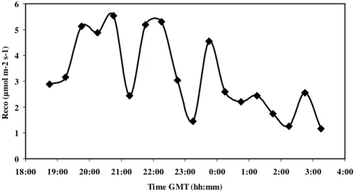
The temporal variability ofReco is usually attributed to temperature and soil water con-5

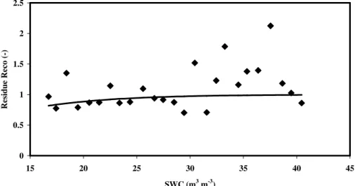
tent variation (Carlyle and Ba Than, 1988; Richardson et al., 2006b). To separate the influence of these two environmental factors, the periods without any water soil stress (Sect. 2.4) are selected to analyse the temperature effect with a Q10 function. The regression is performed withT s10as explained above. After computing the residues of this regression on all theReco values, they are used to simulate SWC impact with a 10

Gompertz function (Janssens et al., 2003):

f(SWC)₌exp (₋exp (a₋b_·SWC)) (2)

whereaand bare two parameters. TheReco complete function (multiplication of the

Q10 and Gompertz functions) is compared to the data to indicate the degree of tem-poral variability explained by T s₁₀ and SWC. When this procedure is applied on the 15

DSEFR and DSIFR half-hour data, the determination coefficients (r2) are very low (re-spectively 0.012 and 0.015) reflecting the fact that other factors thanT s10 and SWC are the major causes of the temporalReco variability. The evolution of the microbial population, soil carbon content available or root and aerial biomass can be evoked but their variation rate is too low compared to the short-term measurement variation 20

(Fig. 2). The change in footprint seems to be a more likely candidate as it could happen between two consecutives half-hours. However, this hypothesis implies a noteworthy ecosystem spatial heterogeneity and it is not apparently the case for the Hesse site that has a reasonably homogenous vegetation type and age. To give some indications about the possible impact of footprint changes on Reco temporal variability, we se-25

(13)

BGD

4, 4197–4228, 2007

B. Longdoz et al.

Title Page

Tables Figures

◭ ◮

Back Close

Full Screen / Esc

EGU

soil water stress period. These measurements are compared according to their prove-nance from a geographical sector. This comparison cannot completely replace a full analysis combining footprint model and detailed map of soil respiration but this map is not yet available. Moreover, the subdivision in patches with homogeneous soil respira-tion that would result from this procedure will probably lead, in the DSEFR case, to a 5

too low number of data per patch to investigate the temperature and soil water impact for many patches. Our Reco comparison between the geographical sectors shows differences. The more evident one appears when the East-Southeast sector (wind di-rection between 75◦_{and 155}◦_{) is compared to the sector including the other wind}

direc-tions. The ecosystem in the East-Southeast sector (meanReco=6.01µmol m−2_s−1₎ 10

produces significantly more CO₂(p=0.034) than the ecosystem out of this zone (mean

Reco₌3.99µmol m−2_s−1_{). When sectors with 45}◦ _{width are determined, the ANOVA}

performed on 5 groups (not enough data between 225◦_–360◦_{) gives a statistically}

sig-nificant difference between the 5 means (p=0.029). The large Reco disparity found with this ANOVA (up to almost 4µmol m−2_s−1_{) has a su}

fficient order of magnitude to 15

potentially explain many of the short-termReco variations. One of the possible causes of this heterogeneity could be the soil respiration dependence on carbon to nitrogen content ratio (C/N). Ngao (2005) has demonstrated this dependence but it could be completely incriminated if the soil C/N map (work in progress) shows a spatial hetero-geneity in agreement with the geographical sectors analysis results.

20

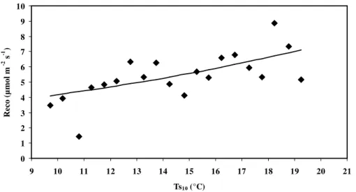
To overcome the spatial heterogeneity problem in the study of the T s₁₀ and SWC influences on Reco, we use the bin-average technique. The bin-averaged Q10 (with

Tref=10◦_{C) and Gompertz regressions are presented in Figs. 3 and 4. Bin-average}

im-proves clearly the goodness of fit (Table 4) withT s₁₀being the main explaining factor for

Reco temporal varibility, as usually found (Richardson et al., 2006b). Reco10 (Table 4) 25

are higher than the value for the equivalent parameter found for the soil respiration, as expected (Rs₁₀ from 1.5 to 2.4µmol m−2_s−1_{, Ngao, 2005) because of the leaves}

(14)

BGD

4, 4197–4228, 2007

B. Longdoz et al.

Title Page

Tables Figures

◭ ◮

Back Close

Full Screen / Esc

EGU

soil plots are low compared to the mean European forests value (69%, Janssens et al., 2001) but there are perhaps not representative of fluxes measured by the EC system. Contrary toReco10, theQ10 value is lower in our study (Table 4) compared to theQ10 estimated for soil (2.55, Ngao, 2005). This is coherent with the contribution of aerial biomass toReco that includes sources less sensible toT s₁₀ than the soil.

5

The quality tests filtering do not lead to a substantial increase of the coefficient of determination of the regressions (for the bin-average and simple cases). Nevertheless, the fact that the regression curves for DSIFR and DSEFR give di_fferences in Reco that range from 7.8% to 16.5% in the 5◦_C–20◦_C _{T s}

10 interval, proves that the data eliminated by this filtering are not evenly distributed.

10

3.4 Gross primary productivity and net ecosystem exchange

In the two datasets, the GPP is calculated for daytime half-hours showing valid NEE measurements (46.7% for DSEFR and 91% for DSIFR). For each time step, theReco simulated with the parameterisation presented in the previous section is subtracted from the NEE measurement to give GPP. The existence of twoReco parameter sets 15

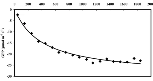
(DSEFR and DSIFR) leads to two GPP time series. The main factor influencing GPP is the photosynthetic photon flux density (PPFD,µmol m−2_s−1_{). This influence is}

pa-rameterised with the Michaelis–Menten relationship adapted by Falge et al. (2001):

GPP= α·PPFD

1−PPFD2000 +

α·PPFD

GPP₂₀₀₀

(3)

whereα is the ecosystem quantum yield (µmol m−2_s−1_{) and GPP}

2000 (µmol m− 2

s−1₎ 20

is the GPP for PPFD equals to 2000µmol m−2_s−1_{. The} _r2 _{of the of the regressions}

(15)

BGD

4, 4197–4228, 2007

B. Longdoz et al.

Title Page

Tables Figures

◭ ◮

Back Close

Full Screen / Esc

EGU

variability in vegetation characteristics comparing to the soil ones). To improve the GPP-PPFD relationship, the bin-average method is also implemented. This allows removing of spatial variability and possible control of other environmental factors like air temperature (T a) or vapour pressure deficit (VPD). The influence of PPFD-GPP appears then extremely clearly (Fig. 5, Table 5). The residues of this parameterisation 5

don’t show any dependence on T aor VPD. This is not surprising in view of the full-leaf 2005 season climate (relatively humid and temperate). Like for Reco, the data selection with the assessment tests do not improve the quality of the regression. This is demonstrated by the relatively low difference (<0.01) between ther2 of the DSIFR and DSEFR regression presented in the Table 5. However, the difference between the 10

parameters obtained with these regressions gives significant variation in GPP between DSIFR and DSEFR cases. The difference goes from 7.1% to 20.6% for PPFD going from 0 to 2050µmol m−2_s−1_{. This result suggests that the data eliminated by the}

filtering possess a common feature.

3.5 TotalReco, GPP and NEE 15

TotalReco, GPP and NEE is calculated for the 2005 full-leaf season by summing the half-hour values in the datasets gap filled with their own parameterisations presented above. The di_fference between the values for DSIFR and DSEFR reveals the impact of the quality tests procedure. The tests application lead to an increase from 740.4 g C m−2_{to 816.1 g C m}−2 _for_R_{eco (10.2% of variation, 75.7 g C m}−2_{). Only a minor part} 20

of this increase (8.3%, 6.3 g C m−2_{) comes from the di}

fference in the environmental factors of the gaps. To estimate this percentage, the gaps of the DSEFR were filled with the parameter set of DSIFR. The rest of the increase is instigated by the change of the parameter sets when the DSEFR are chosen. A similar analysis was performed for the GPP. The GPP generated by DSIFR and DSEFR are, respectively, −1306.5

25

and−1440.6 g C m−2, therefore they let to an assimilation increase of 134.1 g C m−2

(16)

BGD

4, 4197–4228, 2007

B. Longdoz et al.

Title Page

Tables Figures

◭ ◮

Back Close

Full Screen / Esc

EGU

C m−2 _{(10.3%). Surprisingly, the e}

ffect of the environmental factors of the gaps is major (69.5%, 40.5 g C m−2_{). This is explained by the fact that the GPP influence is}

not counterbalanced byReco in opposition with the part induced by the choice of the parameter sets (DSEFR or DSIFR).

It is important to note that the impact of the quality tests on the different CO2fluxes 5

have the same order of magnitude than the expected year to year variations with re-gards to the value already published for forests under similar climate (Aubinet et al., 2002; Carrara et al., 2003). Therefore, application of the quality tests is able to strongly influence the inter-annual analysis. For the NEE (and only for it), this conclusion is still valid even if we do not take into account the data gap filling method, considering that a 10

variation of 40.5 g C m−2_{are only a result from the gap characteristics.}

4 Conclusion

The different tests presented in this paper are rarely applied, together and system-atically, on large datasets. The results for the 2005 Hesse full-leaf season give an overview of their possible contribution. The high percentage of flagged data detected 15

strengthens the importance to continue the work on data selection and data gap fill-ing methods, especially durfill-ing night. The strict data selection does not modify theu* threshold that seems to be relatively constant from year to year even if the forest was heavily thinned during the winter 2004–2005.

One of the expected contributions of the quality tests was the reduction of the un-20

explained short-termReco fluctuations. It is not really the case, because of the large

Reco spatial heterogeneity. Even for a site with homogeneous vegetation like Hesse, theReco temporal variation analysis should probably be studied from the respiration spatial heterogeneity point of view, before focusing on the data quality. In this con-text, the way to proceed seems to first apply a footprint model combined with a soil 25

respiration map before to select the data and study the inter-annual variability.

(17)

BGD

4, 4197–4228, 2007

B. Longdoz et al.

Title Page

Tables Figures

◭ ◮

Back Close

Full Screen / Esc

EGU

data elimination changes the relationship between the CO₂ fluxes and the environ-mental factors. On the other hand, the general features of the gaps differ when the quality tests are applied. Consequently, the gap filling by the parameterisations, using the environmental factors as independent variables, produce differentReco and GPP values for DSEFR and DSIFR. The total Reco, GPP and NEE for the 2005 full-leaf 5

season vary all by about 10%, with more important photosynthesis exchanges, more CO₂ produced by respiration processes and a higher net sequestration when quality tests are applied. The combination of these tests have the potential ability to influence the inter-annual analysis for the CO2 fluxes and they could perhaps give some ele-ments to answer to the usual large discrepancy in the energy balance closure of the 10

eddy covariance sites (Wilson et al., 2002; Kanda et al., 2004). The question of their systematic application on large databases like from the CarboEurope and FLUXNET experiments is legitimate.

Acknowledgements. This work is founded by the project CarboeuropeIP (GOCE-CT2003-505572) of the European Community and by the GIP Ecofor (French Ministry for Environment). 15

References

Aubinet, M., Grelle, A., Ibrom, A., Rannik, ¨U., Moncrieff, J., Foken, T., Kowalski, A., Martin, P. H., Berbigier, P., Bernhofer, C., Clement, R., Elbers, J. A., Granier, A., Grunwald, T., Morgen-stern, K., Pilegaard, K., Rebmann, C., Snijders,W., Valentini, R., and Vesala, T.: Estimates of the Annual Net Carbon and Water Exchange of Forest: The EUROFLUX Methodology, Adv. 20

Ecol. Res., 30, 114–173, 2000.

Aubinet, M., Heinesch, B., and Longdoz, B.: Estimation of the carbon sequestration by a het-erogeneous forest: night flux correction heterogeneity of the site and inter-annual variability, Global Change Biology, 8, 1053–1071, 2002.

Aubinet, M., Berbigier, P., Bernhofer, C., Cescatti, A., Feigenwinter, C., Granier, A., Gr ¨unwald, 25

(18)

BGD

4, 4197–4228, 2007

B. Longdoz et al.

Title Page

Tables Figures

◭ ◮

Back Close

Full Screen / Esc

EGU

Baldocchi, D., Falge, E., Gu, L., Olson, R., Hollinger, D., Running, S., Anthoni, P., Bernhofer, C., Davis, K., Evans, R., Fuentes, J., Goldstein, A., Katul, G., Law, B., Lee, X., Malhi, Y., Meyers, T., Munger, W., Oechel, W., Paw, K. T., Pilegaard, K., Schmid, H. P., Valentini, R., Verma, S., Vesala, T., Wilson, K., and Wofsy, S.: FLUXNET: A New Tool to Study the Temporal and Spatial Variability of Ecosystem-Scale Carbon Dioxide, Water Vapor, and Energy Flux 5

Densities, B. Am. Meteorol. Soc., 82, 2415–2434, 2001.

Black, T. A., Den Hartog, G., Neumann, H. H., Blanken, P. D., Yang, P. C., Russell, C., Nesic, Z., Lee, X., Chen, S. G., Staebler, R., and Novak, M. D.: Annual cycles of water vapour and carbon dioxide fluxes in and above a boreal aspen forest, Global Change Biol., 2, 219–229, 1996.

10

Carlyle, J. C. and Ba Than, U.: Abiotic controls of soil respiration beneath an eighteen-year-old Pinus radiata stand in south-eastern Australia, J. Ecol., 76, 654–662, 1988.

Carrara, A., Kowalski, A. S., Neirynck, J., Janssens, I. A., Curiel Yuste, J., and Ceulemans, R.: Net ecosystem CO₂exchange of mixed forest in Belgium over 5 years, Agric. For. Meteorol., 119, 209–227, 2003.

15

Falge, E., Baldocchi, D., Olson, R., Anthoni, P., Aubinet, M., Bernhofer, C., Burba, G., Ceule-mans, R., Clement, R., Dolman, H., Granier, A., Gross, P., Grunwald, T., Hollinger, D., Jensen, N. O., Katul, G., Keronen, P., Kowalski, A., Lai, C. T., Law, B. E., Meyers, T., Mon-crieff, H., Moors, E., Munger, J. W., Pilegaard, K., Rannik, U., Rebmann, C., Suyker, A., Ten-hunen, J., Tu, K., Verma, S., Vesala, T., Wilson, K., and Wofsy, S. C.: Gap filling strategies 20

for defensible annual sums of net ecosystem exchange, Agric. For. Meteorol., 107, 43–69, 2001.

Feigenwinter, C., Bernhofer, C., and Vogt, R.: The influence of advection on the short term CO₂ budget in and above a forest canopy, Bound.-Lay. Meteorol., 113, 201–224, 2004.

Finnigan, J. J., Clements, R., Malhi, Y., Leuning, R., and Cleugh, H.: A re-evaluation of long-25

term flux measurement techniques. Part I: averaging and coordinate rotation, Bound.-Lay. Meteorol., 107, 1–48, 2003.

Foken, T. and Wichura, B.: Tools for quality assessment of surface-based flux measurements, Agric. For. Meteorol., 78, 83–105, 1996.

Foken, T., G ¨ockede, M., Mauder, M., Mahrt, L., Amiro, B., and Munger, W.: Post-field data 30

qualtiy control, in: Handbook of Micrometeorology, edited by: Lee, X., Massman, W., and Law, B. E.,, Kluwer, Dordrecht, 181–208, 2004.

(19)

BGD

4, 4197–4228, 2007

B. Longdoz et al.

Title Page

Tables Figures

◭ ◮

Back Close

Full Screen / Esc

EGU

of complex meteorological flux measurement sites, Agric. For. Meteorol., 127(3), 175–188, 2004.

Granier, A., Biron, P., and Lemoine, D.: Water balance, transpiration and canopy conductance in two beech stands, Agric. For. Meteorol., 100, 291–308, 2000a.

Granier, A., Ceschia, E., Damesin, C., Dufr ˆene, E., Epron, D., Gross, P., Lebaube, S., Ledantec, 5

V., Le Goff, N., Lemoine, D., Lucot, E., Ottorini, J. M., Pontailler, J. Y., and Saugier, B.: The carbon balance of a young beech forest, Funct. Ecol., 14, 312–325, 2000b.

Houghton, R. A., Davidson, E. A., and Woodwell, G. M.: Missing sinks, feedbacks, and under-standing the role of terrestrial ecosystems in the global carbon balance, Global Biogeochem. Cycles, 12, 25–34, 1998.

10

Hui, D. F., Wan, S. Q., Su, B., Katul, G., Monson, R., and Luo, Y. Q.: Gap-filling missing data in eddy covariance measurements using multiple imputation (MI) for annual estimations, Agric. For. Meteorol., 121, 93–111, 2004.

Janssens, I. A., Lankreijer, H., Matteucci, G., Kowalski, A. S., Buchmann, N., Epron, D., Pile-gaard, K., Kutsch, W., Longdoz, B., Grunwald, T., Montagnani, L., Dore, S., Rebmann, C., 15

Moors, E. J., Grelle, A., Rannik, U., Morgenstern, K., Oltchev, S., Clement, R., Gudmunds-son, J., Minerbi, S., Berbigier, P., Ibrom, A., Moncrieff, J., Aubinet, M., Bernhofer, C., Jensen, N. O., Vesala, T., Granier, A., Schulze, E. D., Lindroth, A., Dolman, A. J., Jarvis, P. G., Ceule-mans, R., and Valentini, R.: Productivity overshadows temperature in determining soil and ecosystem respiration across European forests, Global Change Biol., 7(3), 269–278, 2001. 20

Janssens, I. A., Dore, S., Epron, D., Lankreijer, H., Buchmann, N., Longdoz, B., Brossaud, J., and Montagnani, L.: Climatic influences on seasonal and spatial differences in soil CO₂ efflux, in: Fluxes of Carbon, Water and Energy of European Forests, edited by: Valentini, R., Springer-Verlag, Berlin, 235–253, 2003.

Kanda, M., Inagaki, A., Letzel, M. O., Raasch, S., and Watanabe, T.: Les study of the en-25

ergy imbalance problem with eddy covariance fluxes, Bound.-Lay. Meteorol., 110, 381–404, 2004.

Kolle, O. and Rebmann, C.: Eddysoft – Documentation of a Software Package to Acquire and Process Eddy Covariance Data, Technical Reports – Max-Planck-Institut f ¨ur Biogeochemie, 10, 88, 2007.

30

Law, B. E., Ryan, M. G., and Anthoni, P. M.: Seasonal and annual respiration of a ponderosa pine ecosystem, Global Change Biol., 5, 169–182, 1999.

(20)

BGD

4, 4197–4228, 2007

B. Longdoz et al.

Title Page

Tables Figures

◭ ◮

Back Close

Full Screen / Esc

EGU

impact of chamber disturbances, spatial variability and seasonal evolution, Global Change Biol., 6, 907–917, 2000.

Moffat, A. M., Papale, D., Reichstein, M., Hollinger, D. Y., Richardson, A. D., Barr, A. G., Beck-stein, C., Braswell, B. H., Churkina, G., Desai, A. R., Falge, E., Gove, J. H., Heimann, M., Hui, D., Jarvis, A. J., Kattge J., Noormets, A., and Stauch, V. J.: Comprehensive compar-5

ison of gap-filling techniques for eddy covariance net carbon fluxes, Agric. For. Meteorol., 147(3–4), 209–232, 2007.

Murtaugh, P. A.: Simplicity and complexity in ecological data analysis, Ecology, 88(1), 56–62, 2007.

Nakai, T., van der Molen, M. K., Gash, J. H. C., and Kodama, Y.: Correction of sonic anemome-10

ter angle of attack errors, Agric. For. Meteorol., 136, 19–30, 2006.

Ngao, J.: Determinism of ecosystem respiration in a beech forest, Ph.D. Thesis, University Henri Poincar ´e Nancy I, 2005.

Papale, D., Reichstein, M., Aubinet, M., Canfora, E., Bernhofer, C., Kutsch, W., Longdoz, B., Rambal, S., Valentini, R., Vesala, T., and Yakir, D.: Towards a standardized processing of Net 15

Ecosystem Exchange measured with eddy covariance technique: algorithms and uncertainty estimation, Biogeosciences, 3, 571–583, 2006,

http://www.biogeosciences.net/3/571/2006/.

Paw, U. K. T., Baldocchi, D. D., Meyers, T. P., and Wilson, K. B.: Correction of eddy-covariance measurements incorporating both advective effects and density fluxes, Bound.-Lay. Meteo-20

rol., 97, 487–511, 2000.

Rebmann, C., G ¨ockede, M., Foken, T., Aubinet, M., Aurela, M., Berbigier, P., Bernhofer, C., Buchmann, N., Carrara, A., Cescatti, A., Ceulemans, R., Clement, R., Elbers, J. A., Granier, A., Grunwald, T., Guyon, D., Havrankova, K., Heinesch, B., Knohl, A., Laurila, T., Long-doz, B., Marcolla, B., Markkanen, T., Miglietta, F., Moncrieff, J., Montagnani, L., Moors, E., 25

Nardino, M., Ourcival, J. M., Rambal, S., Rannik, ¨U., Rotenberg, E., Sedlak, P., Unterhuber, G., Vesala, T., and Yakir, D.: Quality analysis applied on eddy covariance measurements at complex forest sites using footprint modelling, Theor. Appl. Climatol., 80, 121–141, 2005. Reichstein, M., Falge, E., Baldocchi, D., Papale, D., Aubinet, M., Berbigier, P., Bernhofer, C.,

Buchmann, N., Gilmanov, T., Granier, A., Gr ¨unwald, T., Havr’ankov’a, K., Ilvesniemi, H., 30

(21)

BGD

4, 4197–4228, 2007

B. Longdoz et al.

Title Page

Tables Figures

◭ ◮

Back Close

Full Screen / Esc

EGU

net ecosystem exchange into assimilation and ecosystem respiration: review and improved algorithm, Global Change Biol., 11, 1424–1439, 2005.

Richardson, A. D., Hollinger, D. Y., Burba, G. G., Davis, K. J., Flanagan, L. B., Katul, G. G., William Munger, J., Ricciuto, D. M., Stoy, P. C., Suyker, A. E., Verma, S. B., and Wofsy, S. C.: A multi-site analysis of random error in tower-based measurements of carbon and energy 5

fluxes, Agric. For. Meteorol., 136, 1–18, 2006a.

Richardson, A. D., Braswell, B. H., Hollinger, D. Y., Burman, P., Davidson, E. A., Evans, R. S., Flanagan, L. B., Munger, J. W., Savage, K., Urbanski, S. P., and Wofsy, S. C.: Comparing simple respiration models for eddy flux and dynamic chamber data, Agric. For. Meteorol., 141, 219–234, 2006b.

10

Ruppert, J., Mauder, M., Thomas, C., and L ¨uers, J.: Innovative gap-filling strategy for annual sums of CO₂net ecosystem exchange, Agric. For. Meteorol., 138, 5–18, 2006.

Schuepp, P. H., Leclerc, M. Y., MacPherson, J. I., and Desjardins, R. L.: Footprint prediction of scalar fluxes from analytical solutions of the diffusion equation, Bound.-Lay. Meteorol., 50, 355–373, 1990.

15

Soegaard, H., Jensen, N. O., Boegh, E., Hasager, C. B., Schelde, K., and Thomsen, A.: Carbon dioxide exchange over agricultural landscape using eddy correlation and footprint modelling, Agric. For. Meteorol., 114, 153–173, 2003.

Staebler, R. M. and Fitzjarrald, D. R.: Observing subcanopy CO₂advection, Agric. Forest Me-teorol., 122, 139–156, 2004.

20

Vickers, D. and Mahrt, L.: Quality control and flux sampling problems for tower and aircraft data, J. Atmos. Oceanic Technol., 14, 512–526, 1997.

Wilson, K., Goldstein, A., Falge, E., Aubinet, M., Baldocchi, D., Berbigier, P., Bernhofer, C., Ceulemans, R., Dolman, A. J., Field, C., Grelle, A., Ibrom, A., Law, B. E., Kowalski, A., Meyers, T., Moncrie_ff, J., Monson, R., Oechel, W., Tenhunen, J., Valentini, R., and Verma, 25

S.: Energy balance closure at FLUXNET sites, Agric. Forest Meteorol., 113, 223–243, 2002. Wilczak, J. M., Oncley, S. P., and Stage, S. A.: Sonic anemometer tilt correction algorithms,

(22)

BGD

4, 4197–4228, 2007

B. Longdoz et al.

Title Page

Tables Figures

◭ ◮

Back Close

Full Screen / Esc

EGU

Table 1. Number of half-hours flagged by the di_fferent quality tests and fraction to the total

2005 full-leaf period (MFC corresponds to mass flow controller). The total value corresponds to the number of half-hours flagged by at least one test (not equal to the sum because of data flagged by more than one test).

Quality test _nFlag_%

Anemometer anomalies 120 1.6 CO₂IRGA anomalies 2445 33.3

MFC anomalies 5 0.1

Stationarity 1753 23.9

Footprint 107 1.5

(23)

BGD

4, 4197–4228, 2007

B. Longdoz et al.

Title Page

Tables Figures

◭ ◮

Back Close

Full Screen / Esc

EGU

Table 2.Number of half-hours flagged by the different quality tests concerning the CO₂

anoma-lies and fraction to the total 2005 full-leaf period. The total value corresponds to the number of half-hours flagged by at least one test (not equal to the sum because of data flagged by more than one test).

Quality test _nFlag_%

Spikes 4 0.1

Mean discontinuities 142 1.9 Variance discontinuities 154 2.1 Absolute limits 6 0.1

Skewness 1063 14.5

Kurtosis 2344 31.9

Standard deviation 247 3.4

(24)

BGD

4, 4197–4228, 2007

B. Longdoz et al.

Title Page

Tables Figures

◭ ◮

Back Close

Full Screen / Esc

EGU

Table 3. Characteristics of the Q₁₀ function fit applied on the DataSet Including Flagged

Records (DSIFR) and DataSet Excluding Flagged Records (DSEFR) with the bin-average tech-nique. Numbers inside parenthesis are standard errors.

Dataset Independent variable Reco₁₀(µmol m−2_s−1₎ _Q

10 R

2

DSIFR T s_Ts10 3.2 (0.21) 1.9 (0.26) 0.554 5 3.4 (0.32) 1.7 (0.34) 0.297

(25)

BGD

4, 4197–4228, 2007

B. Longdoz et al.

Title Page

Tables Figures

◭ ◮

Back Close

Full Screen / Esc

EGU

Table 4. Characteristics of the Q₁₀ and Gompertz functions fit applied (with bin-average

technique) on DataSet Including Flagged Records (DSIFR) and DataSet Excluding Flagged Records (DSEFR). The data are selected regarding to theu* threshold. Numbers inside paren-thesis are standard errors.

Function Dataset Reco₁₀(µmol m−2_s−1₎ _Q

10 R

2

Q10 _DSEFRDSIFR 3.7 (0.32)_{4.2 (0.31)} 1.9 (0.31)_{1.8 (0.28)} _0.4470.44

a b R2

(26)

BGD

4, 4197–4228, 2007

B. Longdoz et al.

Title Page

Tables Figures

◭ ◮

Back Close

Full Screen / Esc

EGU

Table 5. Characteristics of the Michaelis-Menten function fit applied (with bin-average

tech-nique) on DataSet Including Flagged Records (DSIFR) and DataSet Excluding Flagged Records (DSEFR). The data are selected regarding to theu* threshold. Numbers inside paren-thesis are standard errors.

Dataset α GPP₂₀₀₀ R2

DSIFR −0.060 (0.0024) −23.0 (0.29) 0.99

(27)

BGD

4, 4197–4228, 2007

B. Longdoz et al.

Title Page

Tables Figures

◭ ◮

Back Close

Full Screen / Esc

EGU

Fig. 1a.

Fig. 1a. Example of high frequency records of CO₂ concentration (16 May 18:30 GMT) with

(28)

BGD

4, 4197–4228, 2007

B. Longdoz et al.

Title Page

Tables Figures

◭ ◮

Back Close

Full Screen / Esc

EGU

Fig. 1b. Example of high frequency record of CO₂ concentration (18 July 22:00 GMT) with

(29)

BGD

4, 4197–4228, 2007

B. Longdoz et al.

Title Page

Tables Figures

◭ ◮

Back Close

Full Screen / Esc

EGU

0 1 2 3 4 5 6

18:00 19:00 20:00 21:00 22:00 23:00 0:00 1:00 2:00 3:00 4:00

Time GMT (hh:mm)

R

ec

o

(

µ

m

o

l

m

-2

s

-1

)

Fig. 2.Time evolution ofReco (with short-term fluctuations) during the night-time between the

(30)

BGD

4, 4197–4228, 2007

B. Longdoz et al.

Title Page

Tables Figures

◭ ◮

Back Close

Full Screen / Esc

EGU

0 1 2 3 4 5 6 7 8 9 10

9 10 11 12 13 14 15 16 17 18 19 20 21

Ts10 (°C)

R

ec

o

(

µ

m

o

l

m

-2 s -1 )

Fig. 3. Reco dependence on soil temperature at 10 cm depth. The dots correspond to the

(31)

BGD

4, 4197–4228, 2007

B. Longdoz et al.

Title Page

Tables Figures

◭ ◮

Back Close

Full Screen / Esc

EGU 0

0.5 1 1.5 2 2.5

15 20 25 30 35 40 45

SWC (m3 m-3)

R

e

si

d

u

e

R

e

c

o

(

-)

Fig. 4.Influence of the soil water content (first 10 cm depth) on the residues of the relationship

(32)

BGD

4, 4197–4228, 2007

B. Longdoz et al.

Title Page

Tables Figures

◭ ◮

Back Close

Full Screen / Esc

EGU -30

-25 -20 -15 -10 -5 0

0 200 400 600 800 1000 1200 1400 1600 1800 2000

PPFD (µmol m-2 s-1)

G

P

(

µ

m

o

l

m

-2 s -1 )

Fig. 5. GPP dependence on photosynthetic photon flux density. The dots correspond to the