Calendar Effects In The Portuguese Mutual Funds Market

Calendar Effects In The Portuguese

Mutual Funds Market

Márcio Daniel Pereira Barros

Dissertation

Master in Finance

Supervisor:

Prof. Doutor Júlio Fernando Seara Sequeira da Mota Lobão

i

B

N

Márcio Daniel Pereira Barros, born on the 20th of December 1992, in Valença, Viana do Castelo.

In 2010, he enrolled in a Bachelor in Economics in FEP – School of Economics and Management, from which he graduated in 2013.

During the same year, he entered in the Master in Finance in the same institution, having concluded the curricular year with an average grade of 15.

In the course of his academic years, Márcio was also member and part of the Executive Board of AIESEC in FEP.

In 2015, Márcio joined IBM International Services Centre, in Slovakia, where he currently has the position of Financial Analyst.

ii

A

Firstly and most importantly, I want to thank Professor Julio Lobão, for his support since the beginning; this work would not be possible without him. I am deeply grateful for his patience, guidance, share of knowledge and constructive feedback.

I also thank all my family for their total support and concern, especially from my parents. Last but not least, I would like to highlight all the motivation and help provided by my closest friends, who directly or indirectly have contributed to the accomplishment of this goal.

iii

ABSTRACT:

There is a wide range of studies regarding the calendar effects, however very few of those studies are applied to the mutual funds’ performance. This study aims to search the existence of calendar effects (also known as calendar anomalies) in the Portuguese Mutual Funds Market. Since mutual funds can contain other securities besides stocks, it becomes relevant to study this market, filling a lack found in the literature for the Portuguese markets. Additionally, calendar patterns can be helpful for consultants and managers, potentiating their performance; and also for individual investors since they can try to exploit these anomalies.

Our study analyses a sample of the daily shares’ values of the Portuguese mutual funds from 2002 until 2012 and the effects studied are the following: Turn of Year Effect; Turn of Month Effect; Weekday Effect; Holiday Effect; September Effect. We have found some evidence for the Turn of Year Effect and strong evidence for the existence of a Turn of Month Effect. Likewise, there is some evidence that the Holiday effect is also present. Our findings reveal that this market has some lack of efficiency, since these effects could have, in fact, been predicted and they could have given a return of 6% (Turn of Year) or even 26% (Turn of Month).

iv

I

2.1.1. Turn of Year Effect ... 5

2.1.2. Turn of Month Effect ... 7

2.1.3. Weekday Effect ... 7

2.1.4. Holiday Effect ... 9

2.1.5. September Effect ... 9

2.2. Calendar Anomalies in Mutual Funds ... 10

3. DATA AND METHODOLOGY ... 12

3.1. Collection of Data and Sample ... 12

3.2. Methodological Aspects ... 19

3.2.1. Turn of Year Effect ... 20

3.2.2. Turn of Month Effect ... 21

3.2.3. Weekday Effect ... 21

3.2.4. Holiday Effect ... 22

3.2.5. September Effect ... 22

4. EMPIRICAL RESULTS ... 24

4.1. Turn of Year Effect ... 25

4.2. Turn of Month Effect ... 27

4.3. Weekday Effect ... 29

4.4. Holiday Effect ... 34

4.5. September Effect ... 36

4.6. Calendar Anomalies Applied to Stock Funds ... 37

5. CONCLUSIONS ... 39

REFERENCES ... 41

v

I

O

F

Figure 1.1 - Net Assets Of Mutual Funds WorldWide and in Europe, in the period 2003-2013……….………..…2 Figure 1.2 - Evolution of Portuguese Mutual Funds Market, in the Period 1992-2012……….………..…3 Figure 3.1 - Segmentation of Assets Under Management of Portuguese Mutual Funds Market, by Managing Institution, in 2012………13 Figure 3.2 - Categorization of Portuguese Mutual Funds Market, in 2012, based of Assets Under Management………..14

vi

I

O

T

Table 2.1 – Similar Studies in Stock Markets and Mutual Funds………..11

Table 3.1 – Descriptive Statistics of the Sample, by Categories and by Management Entity ………...16

Table 3.2 – Average Returns of the Sample, by Categories, by Management Entity and by Year ………...………...…..17

Table 3.3 – Number of Observations of the Sample, by Categories, by Management Entity and by Year ……….18

Table 4.1 – Turn of Year Effect ………...25

Table 4.2 – Turn of Month Effect ………27

Table 4.3 – Weekday Effect (Monday) ………29

Table 4.4– Weekday Effect (Tuesday) ………30

Table 4.5 – Weekday Effect (Wednesday) ………...31

Table 4.6 – Weekday Effect (Thursday) ……….32

Table 4.7 – Weekday Effect (Friday) ………...33

Table 4.8 – Holiday Effect ………...34

Table 4.9 – Holiday Effect (Segmented by Holiday) ………..35

Table 4.10 – September Effect ……….36

vii

L

A

APFIPP: Associação Portuguesa de Fundos de Investimento, Pensões e Patrimónios CA: Crédito Agrícola

CMVM: Comissão de Mercado de Valores Mobiliários DAX: Deutscher Aktienindex (German Index Fund)

EFAMA: European Fund and Asset Management Association ESAF: Espírito Santo Activos Financeiros

FEI: Fundos Especiais de Investimento FPA: Fundos Poupança Acções

FPR: Fundos Poupança Reforma GDP: Gross Domestic Product INE: Instituto Nacional de Estatística NYSE: New York Stock Exchange OLS: Ordinary Least Squares TOM: Turn of Month

1

1. I

Since the work of Fama (1970) about the Efficient Market Hypothesis, the debate over this issue has been developing exponentially, given place to the birth of a new paradigm (or even subject) in that field, the Behavioural Finance. The latter, apart from the paradigm previously established, defends that economic agents are not fully rational and that there are limits to arbitrage and thus markets will not be efficient. If this is true, then there will be a mispricing and the actual returns will not be the same as the expected returns, this is, there will be abnormal returns (either negative or positive). Given that, an anomaly is referred as a persistent and well known mispricing, as defined by Singal (2004). Hence, each calendar anomaly is also a persistent and well known mispricing, because returns seem to be correlated with some specific periods of the calendar and not only with economic and financial variables. Knowing this, a lot of studies have been carried during the last decades and they had found empirical evidence of this type of anomalies, however the majority of the studies is applied to the national stock markets, leaving a lack of study in other markets, such as the mutual funds market.

With our study, we aim to contribute to the debate of the Efficient Market Hypothesis with some more results. The market we investigate (Portuguese Mutual Funds Market) is one yet not studied and the calendar anomalies are effects of seasonality in the markets, this is, if confirmed they are an evidence that returns can in fact be predicted and they do not follow a random walk, like it is argued by the EMH. Besides this, the study we carry can also be useful for individual investors, given the seasonality that can be exploited by them in order to get profits from it.

The mutual funds is a very special and helpful market for investors that do not have the time or capability to invest in the financial markets; hence, investors’ money can be invested in such markets according to their preferences and that money is managed by professionals, being expected a good performance of those managers. Like it was stated by Gruber (1996), there are other advantages in making such investments: diversification of risk and the possibility of easily change one’s investments. Moreover, there is also the safety given by the legal framework, since this type of investments is usually regulated. On the other hand, there are also disadvantages like the costs with fees and the lower ability to customize one’s investments on his own. Concerning the diversification of risk,

2 there are funds of national stocks, international stocks, international bonds, etc., so there is a wide range of possibilities in which the investors can choose and make their own customised portfolio. Thus, mutual funds are an usual alternative for investors, instead of investing directly in financial markets.

Since the middle of the 20th century that mutual funds started to get relevance in the financial markets and today they play an important role in the finance industry. According to Investment Company Institute (2014), in the United States, in 1950, mutual funds had an amount of total net assets of 2.53 billions of dollars, with just 98 mutual funds and 939.000 shareholder accounts and in 2013 the total amount of net assets of mutual funds was 5936 times higher, distributed by 7707 mutual funds. Also in the US, in 2013 mutual funds held 24% of the US corporate equity and 14% of the US and international corporate bonds. And it seems like this growth is not exclusive from the US and that it has not stopped yet, since worldwide the total net asset of mutual funds had a growth of 111%, just in ten years since 2003. In Europe, this growth is also very present, like we can conclude from Figure 1.1, below.

As we can see in Figure 1.1, in the end of 2013, there was an amount of 9.801 billions of euros allocated to mutual funds in Europe (24.690 millions in Portugal) and EFAMA predicts that this number will be even higher in 2020; they propose three scenarios based on the evolution of the economies and the pessimistic scenario predicts 15.1 trillions of euros and the optimistic one predicts 21.3 trillions of euros.

- € 5.000,00 € 10.000,00 € 15.000,00 € 20.000,00 € 25.000,00 € 2003 2007 2008 2012 2013 Bil lion s o f E u ro s

Figure 1.1 - Net Assets Of Mutual Funds WorldWide

and in Europe, in the period 2003-2013.

Worldwide Europe

3 In Portugal, in the end of 2011, the amount of assets managed by mutual funds was 10817.1 millions of euros, representing 6,14% of 2011 GDP1 _{and 24,9% of the domestic}

stock market capitalization. In the Figure 1.2, we present the evolution of the Portuguese Mutual Funds Market and as we can see, this market had a significant growth in the last decade of the 20th century, both in terms of value and number of funds. Then, in the beginning of the new century, it has occurred a slightly decrease in value and in number of funds; but this trend has been reversed after 2004, with the introduction of Special Mutual Funds in Portugal. Later, with the arrival of the financial crisis, the net asset value of the Portuguese mutual funds market dropped drastically until 2012, reaching half of the value of 2007. However, the number of mutual funds did not altered expressively, what indicates that the average net asset value per mutual fund has also decreased considerably.

Furthermore, besides the high number of studies regarding the calendar anomalies in several national stock markets (including some for Portugal), it seems that other markets are not explored yet, being the mutual funds market one of them.

So in this work, we will study the existence (or not) of calendar anomalies in the national market of mutual funds. For that, the calendar anomalies analysed will be the Turn of Month Effect, the Turn of Year Effect, the Weekday Effect, the Holiday Effect and the September Effect, being these the most common calendar anomalies found in the

1 _{Data from “Instituto Nacional de Estatística”.}

Source: CMVM. 0 50 100 150 200 250 300 350 0 € 5.000 € 10.000 € 15.000 € 20.000 € 25.000 € 30.000 € 35.000 € 1992 1993 1994 1995 1996 1997 1998 1999 2000 2001 2002 2003 2004 2005 2006 2007 2008 2009 2010 2011 2012 Milli o n s o f E u ro s

Figure 1.2 - Evolution of Portuguese Investment Funds

Market, in the Period 1992-2012.

Number of Funds Net Asset Value

4 literature. We will also study in what extent some effects are stronger or weaker within mutual funds managed by the same firm. Additionally, we will also perform the same study to a subsample made only of Portuguese stock funds, in order to compare these results with studies applied to the Portuguese stock market.

In order to accomplish our goal, the data analysed will be the daily shares’ prices of the Portuguese mutual funds from 2002 until 2012. To study the calendar anomalies, we will use the OLS methodology.

Our findings show evidence of the existence of the Turn of Year Effect, Turn of Month Effect and Holiday Effect, being the second the one with the strongest statistical significance.

In Chapter 2, we will discuss the literature about this topic, beginning with the relevant definitions of the anomalies studied, the main theories related to them and then we present some similar studies; finally, still in this chapter, it is done a critical analysis of the literature reviewed. Then in Chapter 3, we will be regarding the Data and Methodology: we will present some data and analysis about our sample and we will discuss some methodological aspects of every step needed to complete our study. In Chapter 4, we present our empirical results divided by calendar effect and in the end a section dedicated to the Portuguese stock funds. Finally, in Chapter 5, we make a summary of our conclusions.

5

2. L

R

In this chapter, we will explain the relevant calendar anomalies for this study, their definitions, their first authors and the main theories that aim to explicate them; for that, most of the studies considered here have been applied to stock markets, since they are the markets where there was more available data and thus there are more studies performed. The section 2.1 is divided into the different calendar anomalies that we will study: for each subsection, it is presented the definition, the empirical studies that tested the anomaly and some explanation theories found in the literature.

After that, we will present some similar studies, analysing their objectives and their methodology. Finally, it is presented a critical analysis of the literature reviewed.

2.1. Calendar Anomalies

2.1.1. Turn of Year Effect

Turn of Year effect is a calendar anomaly related to the months of December and January, more precisely in the last days of December and the first days of January, so, in the literature it is also called January effect or December effect. This effect consists in the abnormal returns of small loser stocks in January, due to the abnormal selling pressure in December; on the other hand, stocks that have performed well in the first eleven months of the year tend to not be sold in December and this way, their prices rise (this part of the effect is also commonly called Christmas effect).

Like it was mentioned by Pettengill (2003), in 1919 there was already allusions to a seasonal effect in January in the stock markets. Rozeff and Kinney (1976) found higher monthly returns in January when comparing to the rest of the year in some periods of their study of NYSE stock market. Keim (1983) was also one of the first to test this effect and he found that abnormal returns of January were higher than in the other months and that there was a correlation between the size of the stock and those abnormal returns; this correlation was always negative, being more intense in January; additionally, he found that the majority of the abnormal returns in January were coming from its first week.

6 Another popular study is the one executed by Singal (2004) where he tested some U. S. stock markets (NYSE, AMEX and NASDAQ) in the period 1963-2001 and found that the January effect has a significant impact in small loser stocks. One more relevant study is the one carried on by Lakonishok and Smidt (1988) where they made an analysis of 90 years of the Dow Jones Industrial Average Index to find calendar anomalies and they found evidence of the Turn of the Year effect too. In contrast, in the study of Silva (2010), it was not found the January effect in the Portuguese stock market.

The main theory beyond this effect is the tax-loss selling, this is, investors would sell small losers in the end of the fiscal year to offset capital gains and this way they would pay less taxes; the winners would not be sold in December, but only in January and thus investors could postpone the taxes payment by one year. Reiganum (1983) proposed this latter explanation for this effect, however he also found controversial empirical data: small stocks that had performed well (and thus would not be sold in December) were also experiencing abnormal returns in January, but not in the first few days though. Furthermore, in a study of this effect in Canada, Berges et al. (1984) found evidence of its existence and until 1973 Canada did not have capital gains taxes; likewise, this seasonal anomaly was found in stock markets like the Australian one where the fiscal year ends in June, so one can conclude this explanation cannot be the applied to all the markets. A different relevant theory is the liquidity hypothesis that states that in the end of the year, investors usually receive extra income and this would lead to higher investment in the beginning of the year (Ritter, 1988); associated with this is the fact that a lot of relevant information about firms is released in that period like it was referenced by Rozeff and Kinney (1976). Finally, the window dressing hypothesis is also accepted to explain this seasonal effect; Haugen and Lakonishok (1988) proposed that portfolio managers would rebalance the securities owned due to the presentation of the year end holdings to investors and in the beginning of the new year they would invest again in small and riskier stocks that were previously owned. In 2007, Anderson et al. have also offered a new explanation, this time based on psychological factors. Singal (2004) also presented a relevant explanation for the persistence of this effect: according to him, this effect persists because of the high trading costs that make the transaction unprofitable and therefore he presents alternative solutions and one of them is investing in mutual funds, since it would require the less amount of fees to capture this effect and make profit from it.

7

2.1.2. Turn of Month Effect

In analogy with the Turn of Year effect, this effect is visible in the last days of a month and in the first days of the following month and it is illustrated by the rise of the stock returns in this period.

Ariel (1987) was one of the first ones to study this effect in the USA stock market and his conclusions go in the way of the abnormal returns during the turn of the month. In order to develop Ariel’s work, Jaffe and Westerfield (1989) applied his study to other four countries (United Kingdom, Canada, Australia and Japan) and in their opinion there is stronger evidence of a “last day of month” effect, since there are significant and large returns in that day. Lakonishok and Smidt (1988) found also evidence of this effect in their 90 year analysis of DJIA index. Silva (2010) has also found statistical significance of this turn-of-month effect for the Portuguese stock market.

In the explanation theories of this effect, the turn-of-month liquidity hypothesis is one of the most relevant and it was proposed by Ogden (1990): this theory argues that the stock raises in the turn of the month are related to cash receipts of investors and thus they would rise the demand for stocks, investing more; hence, it is also establishes a connection between the monetary policy and the stock returns.

2.1.3. Weekday Effect

The weekday effect is reflected through a consistent abnormal returns in some specific days of the week. The most common weekday effect is the weekend effect in which it is verified a large stock returns on Fridays and zero or even negative stock returns on Mondays.

This effect was firstly referred by Cross (1973) in the study where he analyses only Fridays and the following Mondays, for the New York Stock Exchange, however in 1930 the Monday effect was already recognized, as cited by Pettengill (2003). French (1980) also found that the average returns on Mondays were significantly negative in contrast with the other four days of the week, in the United States. Later, Jaffe and Westerfield

8 (1985) studied this effect in other four countries (United Kingdom, Australia, Japan and Canada) and they found evidence of the existence of it; still, for Japan and Australia the lowest returns were found on Tuesdays and not on Mondays. Dubois and Louvet (1996) also executed this study with eleven countries and they found this effect was weakening in the United States, but it was still stronger in Europe, Hong Kong and Canada. Lately, it was also found a correlation between the firm size and this weekend effect: for small firms can be observed the standard weekend effect, whereas for larger firms there is a “reverse” weekend effect (Brusa et al. (2005)). For the case of the Portuguese stock market, the weekday effect was not found, as it was concluded by Silva (2010).

Amongst the several explanations for this effect, the primary one is the short selling, as stated by Singal (2004). The author argues that this effect comes from unhedged short sellers that take a lot of risk and this way they need a close monitoring of their positions to avoid losses; since in non trading hours, they can not perform this monitoring, they become highly exposed to risk, because it can arrive new information to the market and they can not trade; hence, this type of investors would want to close their positions before the end of the trading days, but because of the costs to do that, they would only close their positions on Fridays because the weekend is a period with more hours of non trading, so they will have more risk if they left their positions open. Singal (2004) found evidence of the latter hypothesis, having the stocks with higher level of short selling the stronger presence of this effect; additionally, this author also refers that this effect is more intense with institutional investors since individual investors do not execute short selling that often. Miller (1988) and Lakonishok and Maberly (1990) support a different explanation; individual investors make their financial planning during weekends and become more active on Mondays (mostly with selling orders) and institutional investors would make their planning on Mondays and thus they would be less active in the market; this hypothesis is known as information processing hypothesis. Another factor that can help to explain this effect is the pattern of information flows found by Damodaran (1989): bad news tend to be released on Fridays or during the weekends and this way there is more likely to exist negative returns on the following Mondays. On the other hand, Rystrom and Bensom (1989) suggest a psychological explanation based on the fact that Monday is seen as a “bad day” and investors are less positive and this way they will be more likely to sell and less likely to buy.

9

2.1.4. Holiday Effect

The Holiday effect has on its basis the abnormal positive returns in each day that precedes an holiday.

Fields (1934) was the first to reference this effect on his study applied to DJIA, where he found higher returns on the day preceding a holiday. Later, this study was extended by Lakonishok and Smidt (1988) in their 90 year analysis, where evidence was found again. Kim and Park (1994) also run tests to study the presence of this effect in the United States, United Kingdom and Japan and it was found evidence in the three of them. In addition, Meneu and Pardo (2004) found this effect in the Spanish stock market, as well as Balbina and Martins (2002) found evidence of higher returns the days preceding a public holiday in the Portuguese stock market (Silva (2010) has confirmed this findings for the latter, too).

Meneu and Pardo (2004) also present an explanation for the holiday effect: small investors become afraid of new information that can arrive during the holiday and they would not have the possibility to close their positions, so they close their positions in the pre-holiday day. An alternative explanation was proposed by Frieder and Subrahmanyam (2004): this effect would be caused by the “mood” of the people when a holiday is coming, resulting in a buying pressure.

2.1.5. September Effect

From all the calendar effects referred in the literature, the September effect will be one of the less studied, but that does not mean it can not be relevant. This effect consists in the significant lower returns that the markets present during this month of the year.

In their seasonal analysis to the United Kingdom equity market from 1955 to 1990, Clare, Psaradakis and Thomas (1995) found that September is the month with lower returns; Jacobsen and Zhang (2012) corroborated the study of the previous authors, finding that September is the month with lowest returns in the period 1951-2009. Reutter, Weizsacker

10 and Westermann (2002) also found evidence of this effect in the DAX in the period 1959-1999 and none of the variables that were tested in order to explain it were able to do it. One possible explanation for this effect is related with the arrival of colder seasons and with the shortening of daylight that can lead to a depression effect in the investors (since Hirshleifer and Shumway (2003) have confirmed the impact of cloudy and sunny days on the performance of NYSE stock market, where cloudy days would have a worse performance than in the sunny ones).

2.2. Calendar Anomalies in Mutual Funds

Bearing in mind the literature reviewed, we can state that studies of seasonality regarding mutual funds scarce. Looking at the Table 2.1 below, we can see that the majority of the studies both on stocks and in mutual funds apply the OLS method, so it seems to be the best alternative to study seasonality in mutual funds. Another important remark of the studies applied to mutual funds is the division in sub-categories of mutual funds, since there is a huge heterogeneity in the composition of them. The effect most studied within the mutual funds literature is the Month of the Year and it seems to be one of the most presents in such funds too; but this fact can be related to the available data (commonly monthly data), so in our work we will be able to study other specific effects since we have available daily data.

Hence, in our work, we intend to study the existence of some of the calendar effects studied in the literature reviewed, through the OLS methodology, applied to the Portuguese mutual funds market.

11 Securities Type Authors Anomalies Studied Securities Under Analysis

Type of Data Sample Period Methodology Results

Stocks Georgantopoul os and Tsamis (2012) Day of the week; January; half month; Turn of month; time of the month DAX (Germany); CAC40 (France); ATX (Austria); BVL (Portugal); ASE (Greece) Daily closing prices January 2000 – July 2008 OLS; GARCH (1,1); not adjusted by dividends Turn of month is the most present effect; no evidence of half month effect Silva (2010) Weekday; January; Pre-holiday; Turn-of-month PSI-Geral; PSI20-TR Daily closing prices May 1989 – December 2008; December 1992 – December 2008 OLS; dividends-adjusted Pre-holiday and turn-of-month were the only significant anomalies Lakonishok and Smidt (1988) Monthly; Semimonthly; Weekend; Holiday; End of December; Turn-of-month Dow Jones Industrial Average Daily closing prices 1897 - 1986 OLS; not adjusted by dividends Evidence of Weekend, Turn-of-month, Turn-of-year and Holiday effects Mutual Funds Farinella and Koch (2000) Month of the Year Money Fund Report, IBC Financial Data Inc. Weekly changes in tax-exempt and taxable MMF yields and assets January 1984 – May 1997 OLS (Newey-West correction) Evidence of Turn-of-Year effect; Evidence of Quarters effect Vidal-García and Vidal (2014) Month of the Year

All the mutual funds in the UK, including non-surviving; Bloomberg and Datastream Monthly prices and returns January 1987 – December 2010 OLS Seasonal patterns in January, February, April and May Lin and Chen

(2008) Day of the Week Taiwan Open-End Equity Funds (data obtained from Taiwan Economic Journal)

Daily net asset value January 1986 – June 2006 OLS Evidence of Weekend Effect Gallagher and Pinnuck (2006) Month of the Year Australian open-end mutual funds (University of Melbourne and AIMA) Month-end holdings January 1990 – December 1997

OLS Greater than

normal performance in December

Alves (2014) Quarter of the Year Equity Europe or Equity Eurozone mutual funds (provided by Lipper) Monthly Returns November 2003 – March 2012 OLS Better performance in the first half of

the year (second quarter positively performing and third quarter negatively performing)

12

3. D

A

M

In this chapter, we will expose our data and sample and then we will discuss the methodology applied to each calendar effect. In the first section (Section 3.1), we present and analyse our sample and in the second one (Section 3.2), we explain some general details of the estimations to be performed and then we divided it by calendar effect and explain the specific details of each regression.

3.1. Collection of Data and Sample

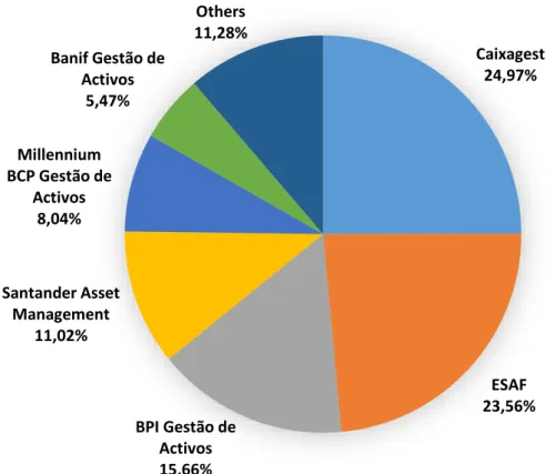
By the end of 2012, there were 12295.3 millions of euros under management by Portuguese mutual funds, what represented a growth of more than 10% since one year before2. This amount was being managed by 17 different companies and as we can observe in Figure 3.1, the three companies with the higher amounts under management were managing more than 60% of the total amount of assets under management in Portugal, divided by 105 mutual funds. It is important to clarify that almost all of the management companies belong to the more relevant banking groups in Portugal. The largest management company (Caixagest) was managing about 25% of the total and the smallest one (Invest Gestão de Activos) was managing 0,1%.

13 By that time, there were 263 funds in Portugal and the biggest one (Espírito Santo Liquidez) had assets under management with a value of 999.4 millions of euros, representing 8,1% of the total amount. The amounts of these funds were being invested mostly in securities (68,5%) and liquidity instruments (20,4%). Within the securities category, the biggest amounts were invested in bonds (34,9% of the total amount), predominantly foreign bonds, followed by shares of other mutual funds (13%), equity (11,1%) and public debt (9%); still in this category, foreign investment represented 42,2% of the total amount invested. Concerning the amounts invested in Portuguese equity, the main targeted companies were Espírito Santo Financial Group (20%), BES (16,8%) and ZON Multimédia (9,4%). Looking at the categorization made by APFIPP (as we can see in Figure 3.2), we can conclude that the majority of the amount managed by Portuguese

Caixagest 24,97% ESAF 23,56% BPI Gestão de Activos 15,66% Santander Asset Management 11,02% Millennium BCP Gestão de Activos 8,04% Banif Gestão de Activos 5,47% Others 11,28%

Figure 3.1 - Segmentation of Assets Under Management

of Portuguese Mutual Funds Market, by Managing

Institution, in 2012.

Source: APFIPP. Others contains: Montepio Gestão de Activos; Barclays Wealth Managers Portugal; Patris Gestão de Activos; Crédito Agrícola Gest; BBVA Gest; MCO2; Popular Gestão de Activos; MNF Gestão de Activos; Dunas Capital – Gestão de Activos; Optimize Investment Partners; Invest Gestão de Activos.

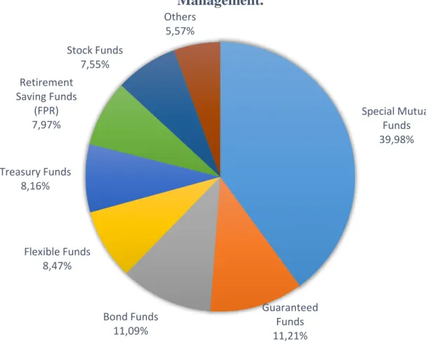
14 mutual funds belonged to Special Mutual Funds; following them, Capital Guaranteed Funds and Bond Funds are the two categories with higher amounts under management; then, Flexible Funds, Treasury Funds, Retirement Saving Funds and Stock Funds comprise all together about 32% of total amount, being the remain amount distributed by smaller categories such as Funds of Funds or Index Funds.

The data for this study is provided by CMVM and by the investment companies that own the Portuguese mutual funds. The sample collected contained the daily closing prices of the shares of the mutual funds in a period of ten years, from 2002 to 2012, amounting to 586743 observations. This data had a reach of 457 funds, from several categories. Given the abovementioned data, some funds had only available monthly or weekly closing prices, so we removed them from our sample; this way, we ended with 390 mutual

Special Mutual Funds 39,98% Guaranteed Funds 11,21% Bond Funds 11,09% Flexible Funds 8,47% Treasury Funds 8,16% Retirement Saving Funds (FPR) 7,97% Stock Funds 7,55% Others 5,57%

Figure 3.2 - Categorization of Portuguese Mutual

Funds Market, in 2012, based of Assets Under

Management.

Source: APFIPP. Others contains: Funds of Funds; Money Market Funds; Balanced Funds; Stock Saving Funds (FPA); Index Funds; Other Funds.

15 funds and the corresponding daily closing prices of its shares. Besides the official holidays, they were also removed from our sample another additional days, the 24th _of

December of each year and the Carnival day of each year, since most of the funds were not traded on these days successively every year.

Thus, our final sample contained 561138 observations in the period from 4 June 2002 until 11 April 2012, comprising 2468 trading days. The average number of trading days per fund is 1461 and the average number of observations per trading day is 231.

In the tables below, we can see a summary of the descriptive statistics of our sample. In Table 3.1, we can see some statistics regarding the returns, like average, median, maximum, minimum and standard deviation and a column regarding the number of funds; we also divided the sample into subsamples using two different criteria: managing institution and categories (regarding the categorization, it was followed the categorization of APFIPP and when this was not available, it was followed the categorization of CMVM). In Table 3.2, we present an extensive analysis of the average returns divided by subsamples, following the criteria mentioned above, and divided by year too. Finally, in Table 3.2, we have an analysis of the number of observations also divided by subsamples following the criteria mentioned and by year.

16

Mean (%) Median (%) Maximum (%) Minimum (%) Standard Deviation No of Funds

TOTAL 0,0006 0,0321 1,6818 -2,0556 0,3166 390

CATEGORIES

Money Market Funds 0,0066 0,0057 0,3462 -0,3389 0,0127 7

Treasury Funds 0,0058 0,0061 1,8940 -1,8891 0,0652 37

Bond Funds -0,0014 0,0050 0,7551 -0,7913 0,0929 54

Stock Funds -0,0040 0,0787 5,5639 -5,9677 0,9149 58

Mixed Funds -0,0007 0,0274 2,3166 -2,7329 0,3892 15

Funds of Funds 0,0011 0,0262 2,4777 -2,6605 0,3333 41

Capital Guaranteed Funds 0,0087 0,0202 2,2379 -6,3621 0,4043 34

Flexible Funds 0,0049 0,0344 3,3666 -3,4792 0,4466 21

Index Funds -0,0037 0,0550 10,1928 -10,4605 1,1897 1

Special Funds (FEI) 0,0013 0,0129 1,7129 -1,5044 0,1290 87

Other Funds -0,0012 0,0066 0,4928 -1,1168 0,0858 3

Stock Saving Funds (FPA) -0,0042 0,0903 6,3347 -7,7455 0,8981 10

Retirement Saving Funds (FPR) 0,0072 0,0155 4,8581 -4,8105 0,1919 22

MANAGING ENTITIES BANIF -0,0058 0,0337 2,2458 -3,0742 0,3915 20 BARCLAYS 0,0049 0,0276 12,1834 -12,5899 0,5941 23 BBVA 0,0012 0,0217 2,2983 -2,2364 0,3434 29 BPI 0,0028 0,0295 3,9580 -2,6955 0,4795 28 BPN -0,0025 0,0244 3,3917 -3,8968 0,4633 9 CA 0,0049 0,0273 2,2065 -2,7978 0,3157 12 CAIXA 0,0017 0,0240 1,2586 -3,1846 0,2865 68 ESAF 0,0028 0,0314 2,7212 -3,1056 0,3852 41 MILLENNIUM -0,0004 0,0286 3,3576 -2,5840 0,4413 42 MONTEPIO 0,0015 0,0410 2,9838 -3,0970 0,4785 28 POPULAR 0,0036 0,0374 2,8014 -2,4604 0,4259 15 SANTANDER 0,0019 0,0212 3,8651 -2,9949 0,5033 56

17 2002 2003 2004 2005 2006 2007 2008 2009 2010 2011 2012 TOTAL -0,0690 0,0309 0,0185 0,0338 0,0262 0,0117 -0,0945 0,0432 -0,0014 -0,0359 0,0503 CATEGORIES

Money Market Funds 0,0078 0,0061 0,0045 0,0040 0,0061 0,0091 0,0109 0,0045 0,0029 0,0099 0,0093 Treasury Funds 0,0079 0,0101 0,0051 0,0045 0,0068 0,0080 -0,0027 0,0063 0,0016 0,0057 0,0258 Bond Funds 0,0158 0,0093 0,0083 0,0056 0,0020 -0,0008 -0,0342 0,0087 -0,0180 -0,0263 0,0784 Stock Funds -0,1886 0,0565 0,0330 0,0782 0,0566 0,0196 -0,2310 0,0995 0,0135 -0,0674 0,0433 Mixed Funds -0,0453 0,0234 0,0093 0,0242 0,0177 0,0052 -0,1106 0,0544 0,0046 -0,0260 0,0613 Funds of Funds -0,0705 0,0234 0,0128 0,0356 0,0178 0,0069 -0,1131 0,0639 0,0211 -0,0357 0,0688 Capital Guaranteed Funds -0,1121 0,0797 0,0453 0,0247 0,0378 0,0146 -0,0330 0,0154 -0,0364 -0,0228 0,0958 Flexible Funds -0,0600 0,0508 0,0159 0,0375 0,0253 0,0168 -0,1130 0,0564 0,0166 -0,0371 0,0517 Index Funds -0,1147 0,0649 0,0662 0,0676 0,1292 0,0793 -0,2870 0,1198 -0,0415 -0,1187 -0,0458 Special Funds (FEI) NA NA 0,0031 0,0150 0,0107 0,0090 -0,0324 0,0139 0,0039 -0,0198 0,0280 Other Funds -0,0012 0,0099 0,0068 0,0060 0,0080 0,0020 -0,0348 -0,0060 -0,0102 -0,0030 0,0184 Stock Saving Funds (FPA) -0,1282 0,0935 0,0741 0,0713 0,1113 0,0555 -0,2916 0,1377 -0,0707 -0,1374 -0,0337 Retirement Saving Funds (FPR) 0,0072 0,0203 0,0124 0,0158 0,0140 0,0120 -0,0437 0,0317 0,0070 -0,0213 0,0655 MANAGING ENTITIES BANIF -0,0765 0,0386 0,0271 0,0379 0,0341 0,0181 -0,1425 0,0272 -0,0136 -0,0503 0,0396 BARCLAYS -0,0172 0,0308 0,0253 0,0240 0,0259 0,0123 -0,0937 0,0512 -0,0030 -0,0337 0,0627 BBVA -0,0625 0,0230 0,0150 0,0251 0,0306 0,0114 -0,0648 0,0328 -0,0089 -0,0212 0,0195 BPI -0,0810 0,0382 0,0205 0,0409 0,0334 0,0102 -0,1108 0,0631 0,0171 -0,0477 0,0394 BPN -0,0496 0,0261 0,0114 0,0128 0,0197 0,0054 -0,1159 0,0477 0,0116 -0,0312 0,0585 CA -0,0571 0,0259 0,0174 0,0275 0,0282 0,0192 -0,0574 0,0350 0,0013 -0,0216 0,0235 CAIXA -0,0647 0,0222 0,0157 0,0411 0,0173 0,0079 -0,0601 0,0241 -0,0117 -0,0235 0,0787 ESAF -0,0509 0,0302 0,0207 0,0268 0,0242 0,0139 -0,1002 0,0555 0,0075 -0,0364 0,0573 MILLENNIUM -0,0895 0,0249 0,0155 0,0462 0,0195 0,0058 -0,1136 0,0474 0,0177 -0,0281 0,0451 MONTEPIO -0,0546 0,0369 0,0191 0,0351 0,0388 0,0180 -0,1278 0,0627 0,0005 -0,0485 0,0425 POPULAR -0,0827 0,0416 0,0214 0,0307 0,0253 0,0292 -0,0843 0,0485 -0,0072 -0,0330 0,0506 SANTANDER -0,0949 0,0336 0,0237 0,0315 0,0289 0,0136 -0,0849 0,0376 0,0010 -0,0224 0,0400

18 2002 2003 2004 2005 2006 2007 2008 2009 2010 2011 2012 TOTAL 25264 43264 46365 50831 57111 61412 66442 65286 63462 64132 17569 CATEGORIES

Money Market Funds 513 899 971 965 982 986 621 636 696 745 207

Treasury Funds 3310 4918 4795 4818 4455 4271 4311 4186 4099 4224 1181

Bond Funds 4890 8982 9399 9349 9988 9774 9676 9256 9110 9234 2433

Stock Funds 6486 11043 11221 11697 12008 12594 12977 13189 13151 13483 3900

Mixed Funds 1560 2629 2715 2687 2578 2392 1980 1994 1999 2897 848

Funds of Funds 4760 8203 8429 8374 8465 7878 7739 5342 5263 5008 1207

Capital Guaranteed Funds 146 245 621 1715 2682 2897 4234 5033 5761 5674 1564

Flexible Funds 581 981 1292 1596 1974 2661 3541 3681 4218 4731 1346

Index Funds 145 248 240 219 215 216 245 248 246 250 71

Special Funds (FEI) NA NA 1018 3126 6598 10199 13557 14081 11638 10658 2835

Other Funds 284 474 582 681 705 707 732 726 728 734 210

Stock Saving Funds (FPA) 1182 1881 2066 2220 2225 2170 2236 2238 2247 2016 497

Retirement Saving Funds (FPR) 1407 2761 3016 3384 4236 4667 4593 4676 4306 4478 1270 MANAGING ENTITIES BANIF 1153 1975 2113 2249 2597 2744 3369 3202 3938 3639 993 BARCLAYS 1280 2470 2979 3444 3441 3952 3740 3985 3722 4033 1181 BBVA 1002 1961 2640 3469 4444 4978 5345 3762 3009 2304 632 BPI 2646 4480 4706 4798 5134 5170 5043 5440 5584 5783 1692 BPN 641 1420 1528 1700 2080 2224 2075 1968 1974 1980 566 CA 1008 1724 1747 1725 1969 2042 2636 2706 2411 2070 568 CAIXA 3381 5371 5417 5775 7464 8424 10013 11064 11672 10466 2861 ESAF 3616 5788 6098 6318 6414 6285 6725 6603 6392 6566 1840 MILLENNIUM 3969 6833 7046 7706 8545 8911 8362 6931 6651 6418 1726 MONTEPIO 2188 3676 3899 4263 4633 5562 6595 6613 6767 6635 1560 POPULAR 1131 1987 2066 2667 2960 2235 2738 2544 2207 2522 769 SANTANDER 2534 4337 4899 5517 6351 7748 8355 8403 7313 8736 2337

19

3.2. Methodological Aspects

Firstly, we study every effect for the overall sample and then we categorize the sample in several samples with the criterion of the managing entity, this is, we create sub-samples for each one of the main managing entities with just the observations of the funds managed by them, since they are more likely to be managed according to the same guidelines/managers.

At the same time, we also need to make the calculations for the daily returns of the mutual funds. To do so, we will apply the natural logarithm of the division of two consecutive observations.

Moving on to the next step, the portfolios of the several categories were built by computing the average yield in each category or sub-sample for each trading day (Farinella and Koch 2000), covering the active funds of the sub-sample present in that day.

Having executed the steps above, the next one shall be the implementation of the regressions. This regressions will have the form of the several studies in the area, this is, making use of dummy variables according to the effect we want to study.

𝑅_𝑖𝑡 = 𝛼_𝑖 + 𝛽_𝑖𝐷_𝑡+ 𝜀_𝑖𝑡

𝑅_𝑖𝑡 stands for the daily return of the sub-sample i in the day t and 𝐷_𝑡 is the dummy variable that assumes the value 1 when the condition we are analysing is verified and 0 otherwise.

Some studies about calendar effects in stock markets also make reference to the effect that dividends can have, but the majority has considered it is not necessary to adjust by dividends and so we will not adjust by some regular payments of some funds, too. Other issue we must take into account when working with mutual funds is the survival bias. However, like it as argued by Lobão and Serra (2007) or Grinblatt and Titman (1989),

20 the impact of survival bias on performance is not significant, so it will not also affect our study since we are working with mutual funds performances.

Since we are dealing with time series, it is very likely we have heteroskedasticity or autocorrelation present so we need to make the necessary adjustments. Although the use logarithmic returns is already in place, we could use a GARCH model to make that correction; however, most of the studies, like the ones performed by Farinella and Koch (2000), Lin and Chen (2008) or Matilde (2014), use the Newey-West correction in order to adjust for heteroskedasticity and autocorrelation, so we become able to make conclusions from the significance tests we run. Thus, in our study we will apply the Newey-West correction to the regressions performed and we will still have asymptotically valid statistical inference.

3.2.1. Turn of Year Effect

For this effect, we followed the methodology applied by Tangjitprom (2011). This author used a regression in which it was set a dummy that would take the value 1 for returns in the trading days between the 25th of December and the 31st of December and another dummy that assumes the same value for returns in the period from the 1st of January until the 8th of January (including the latter). Hence, the regression is the following:

𝑅𝑡 = 𝛼 + 𝛽1𝐷1 + 𝛽2𝐷2+ 𝜀𝑡

Where 𝑅_𝑡 stands for the series of returns studied, the 𝛼 is a constant, the 𝐷₁ is a dummy that assumes the value 1 when the observations refer to the days in the period 25-31 December of each year (and 0 otherwise) and 𝐷2 is another one that assumes the value 1

for observations referring to the period 1-8 January of each year (and 0 otherwise). So, the coefficients of these dummies give us the mean returns of those two periods in relation to the rest of the year.

21

3.2.2. Turn of Month Effect

For this effect, the regression applied is the one applied by Gama (1998) and Silva (2010): a regression including a dummy that takes the value 1 for observations associated to the last trading day of each month and to the following first three trading days of the following month. As a result, we have the following regression:

𝑅_𝑡 = 𝛼 + 𝛽₁𝐷₁+ 𝜀_𝑡

Where 𝑅𝑡 stands for the series of returns studied, the 𝛼 is a constant and the 𝐷1 is a

dummy that assumes the value 1 when the observations refer to the last trading day and to the first three trading days of each month (and 0 otherwise) and this way we can examine if there is significantly different returns from the rest of the trading days.

3.2.3. Weekday Effect

Here, we follow a different approach that is not the most usual amongst the literature and that was discussed by Borges (2009). The author argues we should use equations with only one dummy variable, because if we use several dummies, we are studying if these variables are significant in relation with the one missing and not in relation with other variables present in the equation, but if we study each one of them separately in one regression, we can study if that variable is independently significant. Therefore, we use five simple regressions, one for each weekday:

𝑅_𝑡 = 𝛼 + 𝛽₁𝐷₁+ 𝜀_𝑡

Where 𝑅𝑡 stands for the series of returns studied, the 𝛼 is a constant and the 𝐷1 is a

dummy that assumes the value 1 when the observations refer to the respective weekday and this way we can examine if there is significantly different returns from the rest of the weekdays.

22

3.2.4. Holiday Effect

With this effect, the approach used was the one proposed by Cadsby and Ratner (1991), Meneu and Pardo (2004), Chong et al. (2005) and Coutts, Kaplanidis and Roberts (2000); this approach consists in making a regression that uses just one dummy that assumes the value 1 for observations of trading days before an holiday and 0 otherwise:

𝑅_𝑡 = 𝛼 + 𝛽₁𝐷₁+ 𝜀_𝑡

The Portuguese public official holidays were not subject to change during the period 2002-2012, so the ones studied were the following: New Year (1st _{of January); Holy}

Friday and Easter (variable; they are studied together because the Holy Friday happens always in the Friday preceding Easter, which in turn occurs always on Sundays); Day of Liberty (25th of April); Labour Day (1st of May); Corpus Christi (60 days after Easter); Day of Portugal (10th of June); Assumption Day (15th of August); Implantation of the Republic (5th of October); All Saints Day (1st of November); Restoration of Independence (1st of December); Immaculate Conception (8th of December); Christmas Day (25th of December). The dates of the holidays considered here can be found in Annexes.

Additionally, we analyse each holiday individually to investigate if the effect is stronger with some holidays or not.

3.2.5. September Effect

The September effect was studied computing a simple regression with just one dummy that assumes the value 1 for observations in the months of September and 0 otherwise:

23

3.2.6. Portuguese Stock Funds

Lastly and additionally, we will apply the tests executed for each calendar effect to a sub-sample of our main sub-sample: the Portuguese stock funds. This is done because of two reasons: this sub-sample is composed by funds that invest only in the stock market; there are already similar studies applied to the stock market. Hence, this type of funds are inherently correlated with the stock market and we are able to make comparisons with those past studies.

24

4. E

R

Our results here are presented using the terminology used to explain the methodology in section 3.3. Like it was mentioned, we use the Newey-West correction for every regression performed. For each coefficient, we present the statistical significance if it exists with a level of confidence equal or lower than 10%. The sections are divided by each calendar anomaly studied; additionally, there is one final section dedicated to the study of calendar anomalies in Portuguese stock funds, in order to compare results with similar studies applied to the Portuguese stock market. When we find that a calendar effect is present in the main sample with a level of confidence equal or lower than 10%, we will also demonstrate how much an investor would have profited if he had exploited the anomaly found.

We present the results in the following order: Turn of Year Effect, Turn of Month Effect, Weekday Effect (results for each weekday), Holiday Effect, September Effect and finally the results for the sub-sample of Portuguese stock funds.

25

4.1. Turn of Year Effect

From the results of Table 4.1, we can infer that the Portuguese mutual funds have a better performance in the beginning of the civil years. However, we can not say they perform worse on the last days of the year. Furthermore, in the funds managed by institutions such as Crédito Agrícola Gest, Caixagest or Popular Gestão de Activos this better performance is even stronger.

Another finding of the table above is that the coefficient for the first days of January is always substantially bigger than the one for the last days of December. The “α” coefficient, that represents the average return for days that do not belong to the period 25 December – 8 January, is also considerably lower than the other two coefficients, what confirms the theory of this calendar effect. Regarding the signals of the coefficients of the dummy variables, they are positive as it was expected, indicating positive returns in

𝑅𝑡 (%) 𝛼 𝛽1 𝛽2 Prob (F-statistic) Overall Sample 0.002269 0.024338 0.120083** 0.024147 Banif 0.009421 0.031563 0.147236** 0.026813 Barclays 0.002552 0.025054 0.091295** 0.540579 BBVA -0.002083 0.023137 0.080552** 0.222514 BPI -0.000565 0.021604 0.142282** 0.108942 BPN -0.004066 -0.011127 0.088247** 0.398473 Crédito Agrícola 0.002413 0.052884 0.094443*** 0.057640 Caixa -0.001378 0.042884 0.112587*** 0.012968 ESAF 0.000656 0.025907 0.102302* 0.158175 Millennium -0.003444 0.025823 0.132994** 0.098527 Montepio -0.003039 0.031464 0.181030** 0.026859 Popular 0.001298 -0.005106 0.133426*** 0.098157 Santander -0.001953 0.016083 0.128236** 0.188416

Table 4.1 – Turn of Year Effect

This table presents, by management institution and overall, the results of the estimation of the regression 𝑅𝑡= 𝛼 + 𝛽1𝐷1+ 𝛽2𝐷2+

𝜀𝑡, where 𝑅𝑡 is the daily average return (in percentage) of the sample studied in day t, 𝐷1 is a dummy variable that assumes the value

1 for days belonging to the period 25 December – 31 December (including) of each year and the value 0 otherwise and 𝐷2 is also a

dummy variable that assumes the value 1 for days belonging to the period 1 January – 8 January (including) of each year and the value 0 otherwise. The period studied goes from June 2002 until April 2012 and it comprises the trading days of this period. *, ** and *** represent the estimates of the coefficients that are statistical significant for confidence levels of 10%, 5% and 1%, respectively. Since we have more than one variable dependent, it is also presented the p-value for the test of statistical significance of the whole regression, in the last column. R-squared of Overall Sample regression: 0.003017. Number of observations of Overall Sample regression: 2468.

26 those periods (although this does not verify for BPN or Popular Gestão de Activos, for example). Since this regression has two different independent variables, we also present the p-value of F-statistic, in order to test if the regression is statistically significant overall; hence, concerning the p-values of the regressions (last column of Table 4.1), we can see that the regression applied to the overall sample is significant for a level of confidence of 5%; nevertheless, that does not happen with all the regressions of the managing institutions, despite the second coefficient being always significant.

Hence, if theoretically an investor had exploited this calendar effect, investing in a portfolio of all the Portuguese funds just in the periods 1 January – 8 January of each year (during the period of our sample), he would have got a return of 6,08% in January 2012.

27

4.2. Turn of Month Effect

In the below table, we present the results of the regressions regarding the Turn of Month Effect. Given these results, we can infer that the turn of month effect is very strong in the Portuguese mutual funds, presenting higher returns during the last day of a month and the next three first days of the following month. However, the mutual funds belonging to BPN Gestão de Activos seem to have a weaker turn of month effect. Looking at the coefficients, we can see that the “α” one is always negative, meaning a negative average return for days that are not the last one or one of the first three of the month; on the other hand, for days belonging to that four days period, it seems like the average return of the mutual funds is always positive, confirming the theory about the Turn Of Month Effect. As we can verify, the majority of the coefficients of the dummy variable are statistically significant for a confidence level of 1%, indicating a strong presence of this effect in the Portuguese mutual funds market. Again, using our sample as resource and supposing that theoretically an investor had invested in a portfolio of all the Portuguese mutual funds, in these days of each month during the period in analysis, he would have got a profit of

𝑅𝑡 (%) 𝛼 𝛽1 Overall Sample -0.011274 0.061552*** Banif -0.020169 0.074649*** Barclays -0.006114 0.056920*** BBVA -0.009336 0.048318*** BPI -0.011723 0.074946*** BPN -0.009821 0.038080* Crédito Agrícola -0.003937 0.047734*** Caixa -0.004816 0.033725** ESAF -0.012107 0.079411*** Millennium -0.014605 0.074490*** Montepio -0.014855 0.083190*** Popular -0.007987 0.061732** Santander -0.010091 0.057287**

Table 4.2 – Turn of Month Effect

This table presents, by management institution and overall, the results of the estimation of the regression 𝑅𝑡= 𝛼 + 𝛽1𝐷1+ 𝜀𝑡, where

𝑅𝑡 is the daily average return (in percentage) of the sample studied in day t, 𝐷1 is a dummy variable that assumes the value 1 for

days that are the last trading day of the month or the first three days of the month and the value 0 otherwise. The period studied goes from June 2002 until April 2012 and it comprises the trading days of this period. *, ** and *** represent the estimates of the coefficients that are statistical significant for confidence levels of 10%, 5% and 1%, respectively. R-squared of Overall Sample regression: 0.006042. Number of observations of Overall Sample regression: 2468.

28 about 26,74%, what is a significant high value; so this strengthens our findings that the Turn of Month effect can exist in the Portuguese mutual funds.

29

4.3. Weekday Effect

In this section, we present the results of the Weekday Effect regressions (one table for each weekday), following the order Monday-Friday. However, we can already note that it was not found statistical significance for any of the weekdays, either for the overall sample or for the subsamples.

In the Table 4.3, the results for the Monday effect are presented: for the overall sample, the average return on Mondays was negative and lower than on other days; the same happened with the subsamples, but not all of them since BBVA Gest, BPN Gestão de Activos and ESAF present higher average returns for Mondays than for other weekdays.

The Table 4.4, presenting the results of the regression for the Tuesday effect, allow us to get conclusions similar with the ones for the Monday effect: either for the overall sample,

𝑅𝑡 (%) 𝛼 𝛽1 Overall Sample -0.002001 -0.006955 Banif -0.004910 -0.004729 Barclays -0.004587 -0.001304 BBVA -0.000372 0.001679 BPI -0.005714 -0.014958 BPN -0.003200 0.003585 Crédito Agrícola 0.006190 -0.004561 Caixa 0.003077 -0.006966 ESAF 0.002180 0.005056 Millennium 0.000484 -0.003823 Montepio 0.002071 -0.004370 Popular 0.004601 -0.003982 Santander 0.004241 -0.016393

Table 4.3 – Weekday Effect (Monday)

This table presents, by management institution and overall, the results of the estimation of the regression 𝑅𝑡= 𝛼 + 𝛽1𝐷1+ 𝜀𝑡, where

𝑅𝑡 is the daily average return (in percentage) of the sample studied in day t, 𝐷1 is a dummy variable that assumes the value 1 for

days that are Mondays and the value 0 otherwise. The period studied goes from June 2002 until April 2012 and it comprises the trading days of this period. *, ** and *** represent the estimates of the coefficients that are statistical significant for confidence levels of 10%, 5% and 1%, respectively. R-squared of Overall Sample regression: 0.000080. Number of observations of Overall Sample regression: 2468.

30 either for the subsamples, the average returns on Tuesdays were negative and lower than in the other weekdays (with exception of funds managed by BPN Gestão de Activos and Santander Asset Management).

The results from the Wednesday effect regression are also very similar with the Tuesday ones, like we can see in Table 4.5. Generally, the average returns on Wednesdays were negative and lower than the average returns of other weekdays; however, regarding the subsamples, we again can find exceptions like the funds of Barclays Wealth Managers Portugal, BPI Gestão de Activos and BPN Gestão de Activos, which showed positive and higher returns for Wednesday weekdays.

𝑅𝑡 (%) 𝛼 𝛽1 Overall Sample 0.001197 -0.003011 Banif -0.004440 -0.007128 Barclays 0.006014 -0.005845 BBVA 0.001984 -0.010136 BPI 0.002837 -0.000629 BPN -0.003689 0.006093 Crédito Agrícola 0.006360 -0.005483 Caixa 0.002169 -0.002498 ESAF 0.005091 -0.009491 Millennium 0.000437 -0.003633 Montepio 0.002403 -0.006097 Popular 0.004671 -0.004152 Santander 0.000408 0.002666

Table 4.4– Weekday Effect (Tuesday)

This table presents, by management institution and overall, the results of the estimation of the regression 𝑅𝑡= 𝛼 + 𝛽1𝐷1+ 𝜀𝑡, where

𝑅𝑡 is the daily average return (in percentage) of the sample studied in day t, 𝐷1 is a dummy variable that assumes the value 1 for

days that are Tuesdays and the value 0 otherwise. The period studied goes from June 2002 until April 2012 and it comprises the trading days of this period. *, ** and *** represent the estimates of the coefficients that are statistical significant for confidence levels of 10%, 5% and 1%, respectively. R-squared of Overall Sample regression: 0.000015. Number of observations of Overall Sample regression: 2468.

31 With the results of the Thursday effect (presented in Table 4.6), there is a different trend in the average returns: Thursday average returns were, in general, positive and higher than on other weekdays. But this is not a rule to the subsamples of the managing institutions, since five of them still presented Thursday average returns that were negative and lower than in other weekdays.

𝑅𝑡 (%) 𝛼 𝛽1 Overall Sample 0.001528 -0.004581 Banif -0.003926 -0.009492 Barclays 0.009379 0.022293 BBVA 0.000297 -0.001629 BPI 0.001843 0.004266 BPN -0.002593 0.000572 Crédito Agrícola 0.006785 -0.007465 Caixa 0.002105 -0.002139 ESAF 0.003581 -0.001880 Millennium 0.001105 -0.006851 Montepio 0.001535 -0.001701 Popular 0.004974 -0.005570 Santander 0.003924 -0.014672

Table 4.5 – Weekday Effect (Wednesday)

This table presents, by management institution and overall, the results of the estimation of the regression 𝑅𝑡= 𝛼 + 𝛽1𝐷1+ 𝜀𝑡, where

𝑅𝑡 is the daily average return (in percentage) of the sample studied in day t, 𝐷1 is a dummy variable that assumes the value 1 for

days that are Wednesdays and the value 0 otherwise. The period studied goes from June 2002 until April 2012 and it comprises the trading days of this period. *, ** and *** represent the estimates of the coefficients that are statistical significant for confidence levels of 10%, 5% and 1%, respectively. R-squared of Overall Sample regression: 0.000035. Number of observations of Overall Sample regression: 2468.

32 Finally, concerning the Friday effect, as it is shown in Table 4.7, we can conclude that Friday average returns were positive and always higher than in other days. BPN Gestão de Activos was the only subsample of funds to exhibit negative average returns on these weekdays. 𝑅𝑡 (%) 𝛼 𝛽1 Overall Sample -0.000423 0.005141 Banif -0.009672 0.019156 Barclays 0.000995 0.019441 BBVA -0.000018 -0.000080 BPI 0.004149 -0.007219 BPN -0.000742 -0.008740 Crédito Agrícola 0.005481 -0.001067 Caixa 0.000780 0.004484 ESAF 0.003662 -0.002328 Millennium -0.001204 0.004618 Montepio 0.000858 0.001671 Popular 0.001709 0.010378 Santander -0.001553 0.012519

Table 4.6 – Weekday Effect (Thursday)

This table presents, by management institution and overall, the results of the estimation of the regression 𝑅𝑡= 𝛼 + 𝛽1𝐷1+ 𝜀𝑡, where

𝑅𝑡 is the daily average return (in percentage) of the sample studied in day t, 𝐷1 is a dummy variable that assumes the value 1 for

days that are Thursdays and the value 0 otherwise. The period studied goes from June 2002 until April 2012 and it comprises the trading days of this period. *, ** and *** represent the estimates of the coefficients that are statistical significant for confidence levels of 10%, 5% and 1%, respectively. R-squared of Overall Sample regression: 0.000043. Number of observations of Overall Sample regression: 2468.

33 Finalizing this section, although we did not find statistical significance for any regression, the average returns found for each weekday could confirm the existence of a weekend effect in the overall sample.

𝑅𝑡 (%) 𝛼 𝛽1 Overall Sample -0.001301 0.009602 Banif -0.006340 0.002433 Barclays 0.003305 0.007826 BBVA -0.002054 0.010236 BPI -0.000975 0.018705 BPN -0.002165 -0.001578 Crédito Agrícola 0.001547 0.018824 Caixa 0.000237 0.007245 ESAF 0.001486 0.008652 Millennium -0.002241 0.009896 Montepio -0.000911 0.010622 Popular 0.003173 0.003413 Santander -0.002293 0.016402

Table 4.7 – Weekday Effect (Friday)

This table presents, by management institution and overall, the results of the estimation of the regression 𝑅𝑡= 𝛼 + 𝛽1𝐷1+ 𝜀𝑡, where

𝑅𝑡 is the daily average return (in percentage) of the sample studied in day t, 𝐷1 is a dummy variable that assumes the value 1 for

days that are Fridays and the value 0 otherwise. The period studied goes from June 2002 until April 2012 and it comprises the trading days of this period. *, ** and *** represent the estimates of the coefficients that are statistical significant for confidence levels of 10%, 5% and 1%, respectively. R-squared of Overall Sample regression: 0.000150. Number of observations of Overall Sample regression: 2468.

34

4.4. Holiday Effect

From our results shown in Table 4.8, we can assume that there is a holiday effect with a confidence level of just 10%, this is, in the day immediately before a public official holiday, the returns of the Portuguese mutual funds tend to be higher than in the rest of the days.

Regarding the tests made to each main managing firm, only four of them presented this pattern, with a special focus on BBVA Gestão de Activos, whose funds present it with a significance level of 5%, instead of the common 10% of the other regressions. Furthermore, all of the subsamples presented average returns higher in days preceding a holiday than in the rest of the year. Because we found statistical significance, we also made calculations to evaluate how much an investor theoretically would had gained if he had always invested in the days preceding a public holidays during the period of our study and we reached the value of 5.33%.

𝑅𝑡 (%) 𝛼 𝛽1 Overall Sample -0.001532 0.061125* Banif -0.007888 0.059310 Barclays 0.003358 0.042780* BBVA -0.003169 0.089770** BPI -0.000948 0.104730 BPN -0.005042 0.073603 Crédito Agrícola 0.003753 0.043525 Caixa 0.000411 0.036139 ESAF 0.000813 0.069038 Millennium -0.002722 0.069833* Montepio -0.001041 0.063990 Popular 0.000525 0.097726* Santander -0.000554 0.042725

Table 4.8 – Holiday Effect

This table presents, by management institution and overall, the results of the estimation of the regression 𝑅𝑡= 𝛼 + 𝛽1𝐷1+ 𝜀𝑡, where

𝑅𝑡 is the daily average return (in percentage) of the sample studied in day t, 𝐷1 is a dummy variable that assumes the value 1 for

days that precede an official Portuguese public holidays and the value 0 otherwise. The period studied goes from June 2002 until April 2012 and it comprises the trading days of this period. *, ** and *** represent the estimates of the coefficients that are statistical significant for confidence levels of 10%, 5% and 1%, respectively. The public holidays considered here are: New Year (1 January), Easter (variable), Day of Liberty (25 April), Labour Day (1 May), Corpus Christi (variable), Day of Portugal (10 June), Assumption Day (15 August), Implantation of the Republic (5 October), All Saints Day (1 November), Restoration of Independence (1 December), Immaculate Conception (8 December) and Christmas (25 December). R-squared of Overall Sample regression: 0.001318. Number of observations of Overall Sample regression: 2468.