This is a pre-copy-editing, author-produced PDF of an article accepted for publication in Oxford Economic Papers following peer review. The definitive publisher-authenticated
version Ferreira-Lopes A, Sequeira, T.N. and Roseta-Palma C. On the effect of technological progress on pollution: an overlooked distortion in endogenous growth Economic
Oxford Economic Papers
On the Effect of Technological Progress on Pollution: An Overlooked Distortion in
Endogenous Growth
--Manuscript
Draft--Manuscript Number: OEP-D-10-00168R3
Full Title: On the Effect of Technological Progress on Pollution: An Overlooked Distortion in Endogenous Growth
Article Type: Article
Keywords: JEL Classification: O13, O15, O31, O41, Q50
Keywords: Environmental Pollution, R&D, Human Capital, Economic Growth. Corresponding Author: Tiago Neves Sequeira, Ph.D.
Universidade da Beira Interior Covilhã, PORTUGAL All Authors: Alexandra Lopes
Tiago Neves Sequeira, Ph.D. Catarina Roseta-Palma
Abstract: We derive a model of endogenous growth with physical capital, human capital and technological progress through quality-ladders. We introduce welfare decreasing pollution in the model, which can be reduced through the development
of cleaner technologies. From the quantitative analysis of the model, we show clear evidence that the externality from technological progress to pollution considered in this model is sufficiently strong to induce underinvestment in R&D as an outcome of the decentralized equilibrium. An important policy implication of the main result of this article is that it reinforces the case for R&D subsidies.
On the Effect of Technological Progress on Pollution:
An Overlooked Distortion in Endogenous Growth
Abstract
We derive a model of endogenous growth with physical capital, human cap-ital and technological progress through quality-ladders. We introduce welfare-decreasing pollution in the model, which can be reduced through the develop-ment of cleaner technologies. From the quantitative analysis of the model, we show clear evidence that the externality from technological progress to pollution considered in this model is sufficiently strong to induce underinvestment in R&D as an outcome of the decentralized equilibrium. An important policy implication of the main result of this article is that it reinforces the case for R&D subsidies.
JEL Classification: O13, O15, O31, O41, Q50
Keywords: Pollution, R&D, Human Capital, Economic Growth.
1
Introduction
Economic growth is often associated with significant environmental problems, since it is typically accompanied by increases in natural resource use and in undesirable pollutant emissions. The environmental damages unleashed by economic development are not only harmful per se, but also diminish future growth prospects through the degradation of basic productive assets, such as soil, water, and the atmosphere, which are essential for human activities, thus calling into question the sustainability of such growth. It has long been clear that one way out of this conundrum is to develop new technologies, especially those that bring positive economic productivity effects and are also environmentally friendly.
Initially, technical progress was incorporated into growth models exogenously, which showed its potential benefits but did not explain how it occurred. More recently there has been a proliferation of studies of endogenous technical change, which analyse the interaction between choices in the dynamic economic system and technological develop-ment. Some of these studies include environmental variables in the analysis. Smulders [28] is a non-technical summary of the evolution of technology’s role in growth models with natural resources, which points out that the form of technological change is cru-cial and that, given the costs of technological improvements, appropriate regulation is essential to ensure that such change will continue “at a sufficient rate and in the right direction” (pg. 172).1
L¨oschel [17] presents an overview of economic models of environmental policy that incorporate technological change, both exogenous and endogenous. The author em-phasizes the overwhelming evidence for endogenous technological change, especially over a long time horizon, although he highlights the complexities inherent to the in-clusion of such endogeneity in policy models. A more recent survey, focusing on models for climate policy analysis, is Gillingham, Newell, and Pizer [7].
As Jaffe, Newell, and Stavins [13] make clear, both technological innovation and pollution are characterized by market failures leading to a number of well-known ex-ternalities. The negative effects of pollution fall (wholly or in part) on third parties that are not involved in the pollution-producing decision, thus creating an environ-mental externality. As for technology, there are knowledge externalities arising from one firm’s costly investment in new technology, creating beneficial spillovers for other
1Some authors recognize that not all technology is good for the environment. For instance, both
Bovenberg and Smulders [5] and Ikazaki [12] consider distortions in models with pollution-augmenting technological change. More recently, Aghion et al. [1] developed a model that distinguishes between clean and dirty technological change.
firms, since new knowledge has a public-good nature. There may also be adoption externalities if one firm’s use of a technology lowers costs for other firms, through learning effects or network externalities. This double market failure diminishes private incentives for the development of green technologies and strengthens the case for gov-ernment intervention, preferably through the application of combined policies instead of single instruments.2 Contrary to Acemoglu et al. [1] and similar to Ricci [26], we have modelled just one sector of R&D, allowing for a varying effect of technologies in pollution (according to different values of parameters), implying that technologies can be more or less environmently-friendly.
We propose a model of endogenous growth with physical capital, human capital, and technological progress through quality-ladders, to which we add pollution, which can be reduced through technological progress. A paper that is close to ours is Grimaud and Tournemaine [9], which establishes the possibility that an environmental policy promotes growth through its impact on human capital choices. However, our focus is on the R&D sector, which in their model has a simpler production function and does not influence consumption-good production. In fact, the comparison between different externalities relating to the R&D activities would not be possible in a model like theirs. The similarities are that in our model, as in theirs, improvements in technological quality mean fewer emissions, i.e. a cleaner technology, and that the stock of human capital can be put to different, rival, uses. Ikazaki [12] also considers an endogenous growth model with human capital accumulation and pollution. However, his paper does not consider the possibility that technology decreases pollution, nor does it quantify the externalities present in the model. A couple of articles study the impact of clean(er) technologies on growth and the effects of economic policy, namely taxes, on dirty technologies (see e.g. Hart [11] and Koesler [20]). However, none of these papers considers human capital accumulation nor emphasizes quantitative results, as we do.
We show that considering pollution in an endogenous growth model with physical capital, human capital, and R&D introduces distortions, not only on the allocation of
2The authors also mention the problem of incomplete information as another reason for slow
diffusion of better technologies. This market failure may explain, for instance, the widespread under-investment in energy-saving technologies.
resources throughout sectors in the economy, but also on output and capital growth rates. The negative effect of R&D on pollution is an additional externality, which drives the decentralized equilibrium further from the social optimum and adds an extra reason to obtain underinvestment in R&D. In this sense, this paper also contributes to a large literature on the optimality of investments in R&D (see Alvarez-Paleaz and Groth [3] and Jones and Williams [15]). No existing research has introduced the potential externality that derives from the effect of technological progress on pollution and studied it quantitatively in a model with human capital accumulation. This externality is sufficiently strong to induce underinvestment in R&D as an outcome of the decentralized equilibrium, even when typical sources of overinvestment, such as duplication and creative destruction, are considered. The threshold level for the effect of R&D on pollution, above which underinvestment occurs, is relatively low compared with the benchmark value used in previous contributions. An important policy implication is a stronger justification to subsidize R&D, especially when research leads to pollution-decreasing technologies.
The following section presents the model. Section 3 shows the main relationships between variables from a social planner’s point of view. Section 4 presents the decen-tralized equilibrium. Section 5 presents the allocations of human capital and other macroeconomic variables and shows the distortions in the market solution. In Section 6 we calibrate the model and quantify the distortions presented in the previous section, and Section 7 concludes.
2
Model
We build an endogenous growth model with physical and human capital accumu-lation and quality-improving R&D (quality-ladders or vertical R&D), in the line of Segerstrom [27] and Arnold [4], to which we add utility-decreasing pollution. The flow of pollution emissions arises from production in the economy and decreases with the quality index for technologies. The higher is this index, the cleaner is the technology used in the economy.
2.1
Production Factors and Final Goods
2.1.1 Capital Accumulation
The accumulation of physical capital (KY) in the economy arises through production
that is not consumed, and is subject to depreciation: ˙
KY = Y − C − δPKY (1)
where Y denotes production of final goods, C is consumption, and δP represents
depreciation.
Individuals have a given amount of human capital, KH, at each point in time, and
they decide whether to apply it in production, research activities, or schooling. The hours allocated to schooling in turn provide additional accumulation of human capital, according to:
˙
KH = ξHH − δHKH (2)
where HH are school hours, ξ > 0 is a parameter that measures productivity inside
schools, and δH ≥ 0 is the depreciation of human capital.
There is a constraint on total human capital. Since it can be divided into skills for final good production (HY), school attendance (HH), and undertaking R&D (HR),
and by assumption the different human capital activities are not cumulative, we have:
KH = HY + HH + HR (3)
2.1.2 Final Good Production
The final good is produced with a Cobb-Douglas technology:
Y = ADηKYβ, β < 1, η > 0 (4)
where A∈ [0, 1] is an index of the technology production potential for final good pro-duction in a given period of time. Thus A approaches 1 if the economy is approaching its production frontier. D is an index of intermediate goods and is produced using the
following CES technology: D = 1 ∫ 0 ( k i ∑ 0 qkixki )α di 1 α (5)
The elasticity of substitution between intermediate goods is measured by 0 < α < 1.
xi is the intermediate good i and is produced in a differentiated goods sector using
human capital: xi = HYxi, while qki is the quality index of each intermediate good. This means that (4) can be re-written as:
Y = AQη 1−α α R K β YH η Y (6) where QR = 1 ∫ 0 q α 1−α
ki is an aggregate quality index.
2.1.3 R&D Technology
Technological capital, or new qualities of the current technology, QR, are produced in
a R&D sector with human capital employed in R&D labs (HR) and using the current quality (QR). At each point in time, an improvement from the quality level k to
k + 1 occurs with probability υki =
Hλ RQ ϕ R q α 1−α ki
. If an innovation occurs in a given sector i,
quality grows at rate (γ(ki+1)1−αα − γki1−αα )/γki1−αα = γ1−αα − 1. In this quality-ladder environment, when a firm succeeds in developing a new technology, it destroys the profits of the incumbent that is producing the leading-edge technology. In any sector at any time, an innovation occurs with probability υ = HRλQ
ϕ R
QR , so that the aggregate (nonstochastic) quality index will accumulate according to:
·
QR=(γα/(1−α)− 1)HRλQϕR (7)
where 0 < λ ≤ 1 measures duplication (‘stepping-on-toes’) effects and 0 < ϕ < 1 measures the degree of spillover (‘standing-on-shoulders’) externalities in R&D across time, as in Jones [14].
2.2
Consumers
The utility function has the following functional form, similar to Stokey [30]:
U (Ct, Pt) = ∞ ∫ 0 e−ρt [ τ τ − 1(Ct) τ−1 τ − bPκ t ] dt (8)
where ρ is the utility discount rate, b > 0 gives the impact of disutility that a consumer has from pollution , and κ > 1 describes the intensity of the pollution effect on welfare, so that the negative effects of pollution become greater as P increases. Thus high levels of pollution are proportionally more damaging than low levels of pollution.3 P
is pollution, which is equal to:
P = K β YH η YA χ Qϵ R = Y A χ−1 Qϵ+η 1−α α R (9)
Pollution increases with production, especially because we assume χ > 1, which means that higher values of A lead to more production but also more pollution. As the economy approaches the technological frontier, pollution increases. On the other hand, new cleaner technologies may decrease pollution. The effect of QϵR on pollution is crucial, as it means that high technological knowledge decreases pollution.4
3
Optimal Growth
If consumers are affected by a pollution variable they do not control, and firms do not take this impact into account, the decentralized equilibrium will not maximize aggregate welfare. Thus, we must solve a social planner’s problem. In this section we derive the conditions associated with the maximization of (8) subject to the production function (6) as well as the transition equations for the different types of capital (1), (2), and (7).
3The t subscripts are dropped in the remaining sections for ease of notation. 4A sufficient condition is that ϵ > 0.
The problem gives rise to the following current-value Hamiltonian function: H = τ τ − 1C τ−1 τ − b [ KYβHYηAχ Qϵ R ]κ + µP ( AQη 1−α α R K β YH η Y − C − δPKY ) + (10) +µH(ξHH − δHKH) + µR( ( γα/(1−α)− 1)HRλQϕR)
where the µj are the co-state variables for each stock Kj, with j = Y, H, and QR.
Considering choice variables C, A, HY, and HR (and substituting for HH using (3)),
the first-order conditions yield:
∂U ∂C = µP (11) bκχPκ = µPY (12) −bκηPκ HY − µHξ + µPηY HY = 0 (13) µR = µHξ λ (γα/(1−α)− 1) Hλ−1 R Q ϕ R (14) as well as: −µ.P + µP = µPβY KY − δPµP − bκβ Pκ KY (15) . µH µH = ρ + δH − ξ (16) . µR= ρµR− bκϵP κ QR − µPη (1−α α ) Y QR − µR ( γα/(1−α)− 1)ϕHRλQϕ−1R (17) with ∂U ∂C = C− 1
τ representing the marginal utility of consumption. The problem also respects the following transversality conditions for physical capital, human capital, and technological capital, respectively: lim
t→∞µPKPe −ρt = 0, lim t→∞µHKHe −ρt = 0, and lim t→∞µRQRe
−ρt = 0, implying that, in the steady state, (1− 1
τ
)
gY − ρ < 0, which is
guaranteed by τ < 1.
3.1
Optimal Growth Rates
By definition growth rates will be constant, so equation (1) tells us that KY, Y , and
growing at that same rate, respecting equations (2) and (3).
Denote the growth rate of technological capital as gQR and the growth rate of human capital as gKH. From equation (7) we can see that these two growth rates have to obey the following relationship: gKH =
(1−ϕ)
λ gQR.
In the steady-state, we can obtain the output growth rate as follows. From (12) we find bκPκ = µPYχ,which can be substituted into (13) and log-differentiated to yield:
( 1
τ − 1
)
gY + gKH = ξ− ρ − δH (18)
By log-differentiating equation (12) we obtain:
gP = 1 κ ( 1− 1 τ ) gY (19)
From the log-differentiation of equation (6) we obtain:
gY (1− β) = gA+ gKH [( λ 1− ϕ ) ( 1− α α ) + 1 ] η (20)
Also, from the log-differentiation of equation (9) we obtain:
gP = gY + (χ− 1) gA+ ( ϵ + η ( 1− α α ) ( λ 1− ϕ )) gKH (21)
If in this previous equation we substitute (18) and (19) we obtain:
gA= [ 1 κ ( 1− 1τ)− 1 −(1−τ1) (ϵ + η(1−αα ) (1−ϕλ ))] gY − ( ϵ + η(1−αα ) (1−ϕλ )) (ξ− ρ − δH) (χ− 1) (22) Substituting this last expression and also (18) into (20) we obtain the output growth rate: gY∗ = (ξ− δH − ρ) [ η ( 1 +(1−α α ) ( λ 1−ϕ )) + (−ϵ−η( 1−α α )( λ 1−ϕ)) (χ−1) ] [ 1− [ η(1+(1−αα )( λ 1−ϕ))+ (−ϵ−η(1−α α )(1−ϕλ )) (χ−1) (1−β)+ (1 τ +κ−1 κ(χ−1) ) ] ( 1−τ1) ] [ (1− β) + (1 τ+κ−1 κ(χ−1) )] (23)
By substituting this last expression into (18) we obtain the growth rate of human capital: g∗K H = ξ− δH − ρ 1− [ η(1+(1−αα )(1−ϕλ ))+(−ϵ−η( 1−α α )(1−ϕλ )) (χ−1) (1−β)+ (1 τ +κ−1 κ(χ−1) ) ] ( 1− 1τ) (24)
Using the fact that gQR =
λ
1−ϕgKH, we solve for the growth rate of technological capital: g∗QR = λ (1−ϕ)(ξ− δH − ρ) 1− [ η(1+(1−αα )(1−ϕλ ))+(−ϵ−η( 1−α α )(1−ϕλ )) (χ−1) (1−β)+ (1 τ +κ−1 κ(χ−1) ) ] ( 1− 1τ) (25)
Then by substituting equation (23) into (22) we reach the final expression for gA∗, and if we also substitute (23) into (19) we have the final expression for the growth rate of pollution, which is:
g∗P = (ξ− δH − ρ) [ η ( 1 +(1−αα ) (1−ϕλ )) + (−ϵ−η( 1−α α )( λ 1−ϕ)) (χ−1) ] (1 κ ( 1− 1τ)) [ 1− [ η(1+(1−αα )(1−ϕλ ))+(−ϵ−η( 1−α α )(1−ϕλ )) (χ−1) (1−β)+ (1 τ +κ−1 κ(χ−1) ) ] ( 1− 1τ) ] [ (1− β) + (1 τ+κ−1 κ(χ−1) )] (26)
4
Decentralized Equilibrium
In the decentralized equilibrium both consumers and firms make choices that maximize, respectively, their own felicity or profits. Consumers maximize their intertemporal utility function: ∞ ∫ 0 e−ρt [ τ τ − 1(Ct) τ−1 τ − bPκ ] dt
subject to the budget constraint:
.
where a represents the family physical assets, r is the return on physical capital, and
WH is the market wage. The market price for the consumption good is normalized
to 1. Since it is making an intertemporal choice, the family also takes into account equation (2) which represents human capital accumulation.5
The markets for purchased production factors are assumed to be competitive. From the substitution of the technological index (A) from equation (9) into equation (6) we have: Y = Kβ( χ−1 χ ) Y H η(χ−1χ ) Y Q (η1−αα +χϵ) R P 1 χ (28)
From the problem of the representative firm that produces the final good, we know that returns on production are as follows:
WH = η ( χ−1 χ ) Y HY (29) r = β ( χ−1 χ ) Y KY , (30)
However, in the absence of government intervention there is no market price for P , thereby ensuring that there will be an externality from pollution.
Each firm in the intermediate goods sector owns an infinitely-lived patent for selling its variety xi. Producers of differentiated goods act under monopolistic competition
in which they sell their own variety of the intermediate capital good xi and maximize
operating profits, πi:
πi = (pi− wH)xi, (31)
where pi denotes the price of intermediate good i and wH is the unit cost of xi. The
demand for each intermediate good results from the maximization of profits in the final goods sector. Profit maximization in this sector implies that each firm charges a price of:
pi = p = wH/α. (32)
5See Appendix A for the first-order conditions of the consumer problem. Transversality conditions
After insertion of equations (32) and (29) into (31), profits can be rewritten as: π = (1− α)η ( χ−1 χ ) q α 1−α ki Y QR (33) Let ν denote the value of an innovation, defined by:
νt= ∫ ∞ t e−[R(τ)−R(t)]π(τ )dτ , where R(τ ) = ∫ t 0 r(τ )dτ . (34)
Taking into account the cost of an innovation as determined by equation (7), free-entry in R&D implies that,
WHHR= ν HRλQϕR q α 1−α ki if Q·R > 0 (HR> 0); (35) WHHR> ν Hλ RQ ϕ R q α 1−α ki if Q·R = 0 (HR= 0). (36)
Finally, the no-arbitrage condition requires that investing in patents has the same return as investing in bonds:
· ν
ν = (r− δP)− π/ν + υki. (37)
The free-entry condition also means that νν· = w·H
wH − ϕ · QR QR + (1− λ) · HR HR. This fully describes the economy.
4.1
Growth Rates in the Decentralized Equilibrium
In the market steady state, we can obtain the human capital growth rate of the decentralized equilibrium as follows. By using equation (51) and replacing it in
gµ′
H = gµa + gWH which we obtain by (49), we find .
µa
µa = ρ + δH − ξ − gWH. From (29) we have gWH = gY − gKH. Substituting this last equation in the previous one and introducing both in−1τgY =
.
µa
µa which we find in (48) we arrive at: (
1
τ − 1
)
By log-differentiating the production function (28), using the fact that gQR = λ 1−ϕgKH we have: gY [ 1− β ( 1− 1 χ )] = gKH [( λ 1− ϕ ) ( η1− α α + ϵ χ ) + η ( χ− 1 χ )] + 1 χgP (39)
The log-differentiation of equation (9) and some rearrangements returns:
gP = gY − [( ϵ + ( η1− α α )) ( λ 1− ϕ )] gKH (40)
Substituting (40) into (39), solving for gY and replacing into (38) we obtain the
growth rates of human capital and production in the decentralized equilibrium:
gDEK H = ξ− δH − ρ 1− [ η (1−β) ( 1 + ( λ 1−ϕ ) (1−α α ))] ( 1− 1τ) (41) gYDE = (ξ− δH − ρ) [ η (1−β) [ 1 + ( λ 1−ϕ ) (1−α α )]] 1− [ η (1−β) ( 1 + ( λ 1−ϕ ) (1−α α ))] ( 1− 1τ) (42)
By using the fact that gQR =
λ
1−ϕgKH we solve for the growth rate of technological capital: gDEQ R = ( λ 1−ϕ ) (ξ− δH − ρ) 1− [ η (1−β) ( 1 + ( λ 1−ϕ ) (1−α α ))] ( 1− 1τ) (43)
Substituting (41) and (42) into (40) we obtain the growth rate of pollution in the decentralized equilibrium.
5
Optimality of Human Capital Allocations
The shares of human capital allocated to the different sectors in the social planner framework are: s∗H = HH KH = 1 ξ ( gK∗ H + δH ) (44) s∗R = HR KH = λ η ( ϵ χ + η (1−α α )) ( χ χ−1 ) gQ∗ R ξ− δH + gQ∗R ( (1−ϕ)(λ−1) λ ) s∗ Y (45)
The shares of human capital allocated to the different sectors in the decentralized equilibrium are: sDEH = HH KH = 1 ξ ( gDEK H + δH ) (46) sDER = HR KH = (1−α) (γα/(1−α)−1)g DE QR ξ− δH + gQDER [ (1−ϕ)(λ−1) λ + ϕ + 1 (γα/(1−α)−1) ]sDE Y (47)
The equations presented in this section provide a basis for the comparison of the optimal solution with the decentralized equilibrium solution.6 In fact, this model in-corporates several reasons why the decentralized equilibrium solution may be different from the social planner solution:
• The creative destruction (or business stealing) effect - The probability of success
of an innovation is internalized by the social planner but not by the agents in the decentralized equilibrium. The externality occurs since the individual firm does not internalize the (negative) effects that its own probability of success has on the profits of the other firms. When a firm is successful in developing a new technology it destroys the rents created by the incumbent that is produc-ing the leadproduc-ing-edge technology. The social planner, on the contrary, takes into account that an innovation destroys the social return from the previous inno-vation. An increasing rate of creative destruction reduces the time span during
6A detailed explanation of the calculation of these shares is in Appendix B. In the calibration
which a newly invented technology creates value for the inventor. This is mea-sured by 1/(γα/(1−α)− 1) and increases the R&D effort in the market, favouring overinvestment in R&D.
• Spillovers in R&D - The R&D activity depends on past knowledge. This is a
positive effect that firms do not internalize. It contributes to the sub-optimality of R&D and is measured by ϕ.
• Duplication effects in R&D - Some R&D efforts would be redundant in
compar-ison with others. This effect contributes to a greater effort in the decentralized equilibrium than what the social planner would make, favouring overinvestment in R&D. This is measured by λ.
• Specialization gains from R&D - This externality results from the fact that there
can be a difference between the social gains from having better qualities, which the social planner internalizes, and the private gains from having better qualities, which are the only source of gains that the firm considers. In fact, private and social gains would be equal only by coincidence. Having better qualities available increases production and welfare, which is an effect that is not internalized by firms. It is measured by the comparison of η with α. This comparison dictates whether this externality leads to over or underinvestment in R&D.
• Externality from Pollution - The lower the effect on pollution of the technological
index A, measured by χ, and the greater the effect of the technological quality index QR, measured by ϵ, the higher the allocation of human capital to R&D in
the optimal solution. The main mechanism for the latter is described as follows: an increase in the quality of technologies (with ϵ > 0) causes a decrease in pollution (see equation (9)), which induces a positive effect R&D has on utility through pollution (see equation (8)) - an effect that is neglected by the individual agents, due to the absence of pollution markets, but is incorporated by the social planner. This induces the social planner to increase his preferred allocation of human capital to R&D.
in Alvarez-Paleaz and Groth [3] and Jones and Williams [15]. Reis and Sequeira [23] include all those effects except duplication in a model with human capital accumula-tion. We add to this literature the analysis of the pollution externality. Unlike what occurs in most earlier studies, here, due to the introduction of pollution, growth rates in the social planner solution also deviate from the decentralized equilibrium. How-ever, as we will see below, these deviations are relatively less important than those in shares. As usual in studies seeking to assess the distortions between the social planner and decentralized equilibrium solutions, this evaluation is a quantitative issue. For this reason, we now implement a calibration exercise to evaluate the distortions. In this exercise we will see that the last distortion, linked with pollution, is decisive in obtaining underinvestment in R&D, underscoring the crucial mechanism by which the new technologies decrease pollution, even in comparison with other distortions.
6
Quantitative Results
6.1
Calibration Procedure
In this section, we present and justify the calibrated values used for the parameters in the benchmark economy. For the share of physical capital in final good production, we use the typical value, β = 0.36. For the markup in the differentiated goods sector (1/α), we use, based on Norrbin [19]: Table 3 (Electric Equipment), a value of 1/α = 1.33. We use the output growth rate of Western Europe in the period from 1973 to 2001, reported by Maddison [18] (1.88%), as a base for our calibration exercise. As in Strulik [31], we use the TFP growth rate to estimate the growth rate of R&D, using the facts that gKY = gY and gKH =
1−ϕ
λ gQR. Using the values already defined we reach gQR =
0.006878. Following the approach of Strulik [31], we estimate the innovation parameter
γ such that the lifetime of an innovation is 20 years. This implies γ = 1.043898. For the
elasticity of intertemporal substitution (τ ), we follow Jones et al. [16] in considering
τ = 0.8. We note that this is an important parameter, and therefore confirm that a
value in this range is also empirically supported (see Guvenen [10]).
The discount rate (ρ) is set to 0.01, a value in the range used in the literature. The depreciation rate of physical capital (δP) is also set to reside in a lower bound of the
interval usually seen in the literature (0.01). As it is typical for endogenous growth models with human capital accumulation to consider no depreciation of human capital, we also set δH = 0. Small oscillations in these parameters do not greatly effect our
results, as can be seen in the following section. For the duplication effect (λ) we have followed Strulik [31], Pessoa [21], and others in considering λ = 0.25. As is common in previous literature we set η = 1− β in the benchmark exercise. This value is also an intermediate value for gains of specialization as considered by Jones and Williams [15].
For the spillover effects, we follow Reis and Sequeira [23] and set ϕ = 0.4, which is an appropriate value for models with human capital accumulation, as the authors argue. For the effect of pollution on utility, we have adopted the value used in Stokey [30], κ = 1.2. In order to choose the value of χ, we consider evidence on the empirical relationship between output and pollution. This generally indicates an inverted U-shaped relationship between the level of income and pollution, usually known as the Environmental Kuznets Curve (EKC). However, recent country-specific studies have noted that the relationship between income and pollutants can be almost linear or, for some pollutants, N-shaped. In Roca et al. [24] the EKC hypothesis is rejected and the effect of income on pollution is around 1.2. Akbostanci et al. [2] report that this coefficient for Turkey is about 3.5. From Song et al. [29], we see coefficients from 1.5 to 3, regarding China. Thus, we use a value of χ = 2, within the range of plausible values. Finally, for the effect of technological progress on pollution, ϵ, we use 0.5, implying decreasing returns in influencing pollution. As this parameter governs the externality of technology on pollution, which is the focus of our study, we will perform considerable sensitivity analysis on it.
The productivity of human capital in the human capital accumulation process (ξ) is calibrated according to the condition: gDE
Y = 0.0188. This yields a value for ξ = 0.031207 in the benchmark exercise. We also note that ξ is a reasonable value
compared to values for the same parameter used in the economic growth literature. Table 1 summarizes the benchmark values for calibration.
Table 1 - Parameters Values (Benchmark) Production and Utility
gY β δP τ ρ α
0.0188 0.36 0.01 0.8 0.01 0.75 Human Capital and R&D
ξ δH η λ ϕ γ
0.031207 0 0.64 0.25 0.4 1.043898 Pollution
χ ϵ κ
2 0.5 1.2
6.2
Results for the Benchmark Economy
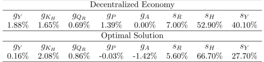
This section presents results for growth rates and shares in the benchmark calibration exercise. Table 2 shows the values obtained for the decentralized economy and, for comparison, the optimal values.
Table 2 - Statistics for the Benchmark Economy Decentralized Economy gY gKH gQR gP gA sR sH sY 1.88% 1.65% 0.69% 1.39% 0.00% 7.00% 52.90% 40.10% Optimal Solution gY gKH gQR gP gA sR sH sY 0.16% 2.08% 0.86% -0.03% -1.42% 5.60% 66.70% 27.70%
Because of the negative effects of pollution, the social planner wishes to deceler-ate the economy, leading to an optimal output growth rdeceler-ate of 0.16%, which is much lower than the 1,88% market equilibrium. However, due to the effect of technological progress on pollution and of human capital on that progress, the social planner solu-tion leads to higher growth rates of human capital and R&D. This implies that the social planner allocates more human capital to human capital production (66.7%) than does the decentralized equilibrium solution (52.9%). Comparing to previous articles that analyzed efficient and market outcomes in endogenous growth models with human capital accumulation, this distortion in the allocation to the human capital sector is new and entirely due to the effect of technological progress on pollution, studied in this article. Due to an especially high creative destruction effect and high duplication effects in this benchmark calibration exercise, the decentralized equilibrium allocates more human capital to R&D than does the social planner.
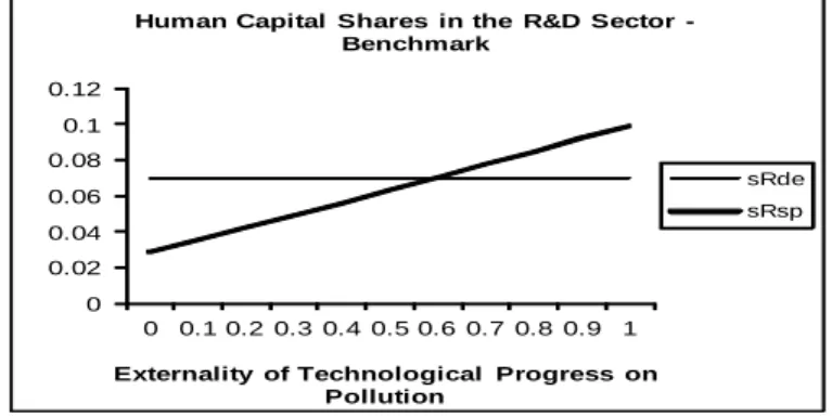
As we introduce a new positive externality of R&D in the model, which is explained by its effect on reducing pollution, we want to know the quantitative importance of this distortion. Thus, we deliberately increase this effect (the parameter ϵ) and observe the impact on the allocations of human capital to the different sectors of the economy (see Fig. 1). 0 0.02 0.04 0.06 0.08 0.1 0.12 0 0.1 0.2 0.3 0.4 0.5 0.6 0.7 0.8 0.9 1
Externality of Technological Progress on Pollution
Human Capital Shares in the R&D Sector -Benchmark
sRde sRsp
Figure 1: Human Capital Allocations to the R&D Sector in the decentralized equilibrium and in the social planner solution - benchmark analysis
We can see that as the externality of R&D in pollution increases, while the decen-tralized equilibrium share to the R&D sector remains constant because this externality does not affect decentralized equilibrium allocations, the social planner share increases. This means that as technology increases its pollution-reduction role, the social planner wishes to allocate more effort to R&D, in order to decrease pollution. This eventually contributes to underinvestment in R&D, which indicates that the pollution externality introduced in this article is capable of overcoming a result of overinvestment in R&D. In particular, the share allocated by the social planner is higher than the share allo-cated in equilibrium above ϵ = 0.69, i.e. above a value that means that a 1% increase in the level of technology led to a reduction in pollution by 0.69%.
6.3
Sensitivity Analysis
In this section, we perform two types of sensitivity analysis. First, we test the variation of the degree of optimality when we introduce variations in a sub-set of our calibrated parameters, those for which there is more uncertainty in the literature. Second, we show the minimum value of ϵ above which underinvestment in R&D occurs, for a
wider variation of each of the parameters in the model. This allows us to generalize our conclusions.
To implement both types of sensitivity analysis we need to establish a set of plausi-ble values for each parameter. The first is the parameter that governs the elasticity of substitution (τ ). While in most theoretical research the elasticity of substitution (1/τ ) is assumed to be around 2, recent empirical evaluations argue that this value can rise to nearly 10 (e.g. Guvenen [10]). In order to perceive how our findings change when the elasticity of substitution rises within plausible values, we consider a value of 1/τ = 5 in the first exercise and then a set of plausible values given by 1/τ ∈ [1.1, 10] . Thereafter, we also consider a smaller duplication effect with λ = 0.5. For the interval of plausible values we follow Jones and Williams [15] to establish that λ ∈ [0.25, 0.99] . For the effect of output on pollution, whose empirical values we have discussed above, we use an upper-bound value of χ = 3.5 and a set of plausible values of χ∈ [1.2, 3.5] . Finally, we consider the possibility that the quality improvements are pollution-increasing, in contrast to what we assumed in the benchmark exercise.7 Thus, we extend the range of possible values for ϵ so it can be negative, and in particular we include values such
that |ϵ| > η1−αα , which would make the net effect of technological progress
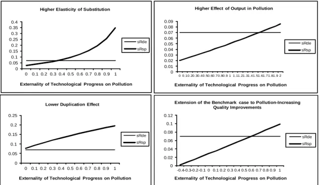
pollution-enhancing. The results of these four cases are presented in Figure 2.
The most important and unexpected result is the effect of the elasticity of substi-tution, shown in the upper left-hand corner. The rise in the elasticity of substitution would increase allocation to the R&D sector by the social planner, meaning that the value of the impact of technology on pollution above which there is underinvestment in R&D decreases. This effect is a complex consequence of the elasticity of substitution on the growth rates in the social planner solution and is also due to the calculation of ξ. For higher values of the elasticity of substitution, closer to the most recent esti-mations, underinvestment results are even more common. For instance for 1/τ = 10, underinvestment always occurs with positive values of ϵ.
The second panel, on the lower left-hand corner, decreases the effect of duplication on R&D. This decreases the factors that lead to overinvestment in R&D and the result is, for all parameter values, underinvestment in R&D. However, the level of
underinvestment varies considerably. For ϵ = 0, we reach a 0.7% difference in the allocation of human capital to the R&D sector between the optimum and the market, yet for ϵ = 1, the difference becomes 12.5%. This is mainly due to the term λη in equation (45). This result makes it straightforward to see that even for higher values of λ > 0.5, underinvestment occurs as long as ϵ > 0.
The third panel, in the upper right-hand corner, illustrates a higher effect of output in pollution, apparently more common in less developed countries as discussed in the previous section. Because of this, the social planner would allocate less effort to R&D (technology also increases pollution due to the link between technology and production) and we need a very high effect of technology in decreasing pollution (ϵ) to overcome that. This is mainly due to the term ϵ/χ in equation (45). The value χ = 3.5 is on the upper bound of the reasonable interval, given the empirical estimations available (see above). Thus, it does not seem appropriate to look for implications of even higher values for the effect of output on pollution. Had we considered a value in the lower bound of the interval of the empirically estimated values, such as χ = 1.2, we would again have concluded that underinvestment would always occur for ϵ > 0.
The lower right-hand corner in the Figure shows additional (negative) values for ϵ, thus including the possibility of a direct and positive effect of technology on pollution. As expected this would decrease the allocation of resources to the R&D sector in the optimal choice even more, since the pollution externality would reinforce the R&D externalities. As in Figure 1, underinvestment in R&D appears when ϵ > 0.7.
0 0.02 0.04 0.06 0.08 0.1 0.12 -0.4-0.3-0.2-0.1 0 0.1 0.2 0.3 0.4 0.5 0.6 0.7 0.8 0.9 1
Externality of Technological Progress on Pollution Extension of the Benchmark case to Pollution-Increasing
Quality Improvements sRde sRsp 0 0.01 0.02 0.03 0.04 0.05 0.06 0.07 0.08 0.09 0 0.10.20.30.40.50.60.70.80.9 1 1.11.21.31.41.51.61.71.81.9 2
Externality of Technological Progress on Pollution Higher Effect of Output in Pollution
sRde sRsp 0 0.05 0.1 0.15 0.2 0.25 0.3 0.35 0.4 0 0.1 0.2 0.3 0.4 0.5 0.6 0.7 0.8 0.9 1
Externality of Technological Progress on Pollution Higher Elasticity of Substitution
sRde sRsp 0 0.05 0.1 0.15 0.2 0.25 0 0.1 0.2 0.3 0.4 0.5 0.6 0.7 0.8 0.9 1 Externality of Technological Progress on Pollution
Lower Duplication Effect
sRde sRsp
Figure 2: Human Capital Allocations to the R&D Sector in the decentralized equilibrium and in the social planner solution - sensitivity analysis
Overall, we reach the conclusion that the pollution externality we introduce in this model can be sufficiently strong to produce results in which there is underallocation of resources to R&D. As with earlier research (e.g. Stokey [30], Reis [22], and Hart [11]) which considered ϵ = 1, for this value almost all exercises in this paper predict market underinvestment in the R&D sector. In fact, for overinvestment in R&D to occur with
ϵ = 1, it would be necessary to have an implausibly high duplication effect (λ < 0.19)
or an implausibly high effect of the technological index on pollution (χ > 2.6).
In the second exercise of sensitivity analysis we consider a set of plausible values for each model parameter, then calculate the minimum ϵ above which there is under-investment in R&D for the minimum and maximum value of each one. We find that for most parameter combinations, the externality that links technology to pollution is sufficiently strong to induce underinvestment in R&D. For the spillover ϕ and the gains from specialization parameter η, we consider the minimum and maximum as in Jones and Williams [15], such that ϕ ∈ [0.457; 0.864]8 and η ∈ [0.196; 1.64]. For the
markup we picked values from Table 3 of Norrbin [19], where for sectors typically as-sociated with specialized goods we have a minimum of 1.008 and a maximum of 1.379 (specialized goods include Machinery, Electric Equipments, and Instruments). For the discount rate ρ, we consider an interval based on different articles, which use values in the interval 0.01 to 0.03 (e.g. Caballero and Jaffe [6]). We did the same for the depreciation rates, which roughly oscillate from 0 to 0.05, but with depreciation rates for human capital that are typically lower than those for physical capital. In fact, we note that most previous endogenous growth models with human capital accumulation assumed a zero depreciation for this type of capital in their calibration. Thus, we set
δP ∈ [0.01; 0.05] and δH ∈ [0; 0.05] . Finally for κ, the effect of pollution in utility,
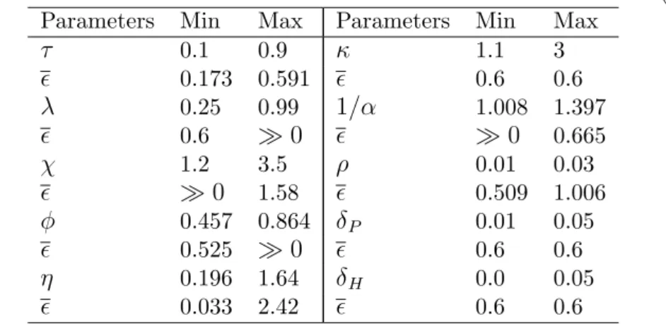
we follow Stokey [30] in considering that that κ > 1 and we use κ ∈ [1.1; 3] . Table 3 presents the threshold levels for the effect of technology in pollution above which there is underinvestment in R&D.
Table 3 - Values for ϵ above which there is underinvestment in R&D (ϵ) Parameters Min Max
τ 0.1 0.9 ϵ 0.173 0.591 λ 0.25 0.99 ϵ 0.6 ≫ 0 χ 1.2 3.5 ϵ ≫ 0 1.58 ϕ 0.457 0.864 ϵ 0.525 ≫ 0 η 0.196 1.64 ϵ 0.033 2.42
Parameters Min Max
κ 1.1 3 ϵ 0.6 0.6 1/α 1.008 1.397 ϵ ≫ 0 0.665 ρ 0.01 0.03 ϵ 0.509 1.006 δP 0.01 0.05 ϵ 0.6 0.6 δH 0.0 0.05 ϵ 0.6 0.6
Note: ≫ 0means that in that case, there is underinvestment for all positive values of ϵ.
Values in Table 3 show that generally, for a large combination of parameters the externality measured by the effect of ϵ is sufficiently strong to induce underinvestment in R&D and this occurs for relatively low values of ϵ. For instance, for the entire realistic interval of values for τ , underinvestment occurs above values of ϵ that oscillate between 0.173 and 0.591. For the realistic interval of the duplication parameter λ underinvestment occurs from values of ϵ above 0.6 until for all positive values of ϵ. consideration that spillovers can be much lower when we consider human capital in the model. For
The wider interval occurs for the gains from specialization, where for values of ϵ above 0.033, underinvestment occurs if η = 0.196 and if η = 1.64 the threshold value of
ϵ is 2.42. Wide intervals appear also for the impact of output in pollution, χ, and
intertemporal discount rate, ρ. The effect of pollution on utility, measured by κ, and the depreciation rates do not change the benchmark threshold of ϵ = 0.6.
The overall conclusion is that for plausible values of the effect of technology in decreasing pollution (ϵ), an increase in this effect is sufficient to induce underinvestment in R&D even when the initial situation is one of overinvestment in R&D, in which creative destruction and duplication effects in R&D are strong. This can be understood as an argument in favour of the existence of subsidies to the R&D sector when the technologies developed in that sector decrease pollution.
7
Conclusion
We derive a complex model of endogenous growth with physical capital, human capital, and technological progress through quality-ladders, to which we add pollution. In particular, we focus on the effect of technological progress in decreasing pollution. This follows the idea of Reis [22], which models technological progress, both exogenously and endogenously, and in which the possibility of discovering a cleaner technology is taken as exogenous. Unlike that author, we model the R&D process as a quality-improving technology in which better qualities are usually cleaner qualities, but the impact they have on pollution may differ considerably.9 Gradus and Smulders [8], Hart [11], and Koesler [20], for instance, also present models in which technological progress reduces pollution. However, none of these authors makes a quantitative evaluation of their models and apart from the much simpler model in Gradus and Smulders [8], no other paper has modelled human capital accumulation as, so that distortions in human capital allocation have not previously been studied. We seek to fill these gaps in the literature.
Examining the optimality of investment in R&D has been the focus of much re-search. However, none introduces the potential externality that derives from the effect
9An extension in which better qualities are more polluting is also presented in the sensitivity
of technological progress on pollution nor studies it quantitatively. We also contribute to this literature.
We derive growth rates for output, human capital, technological progress, and pol-lution resulting from both the decentralized equilibrium and the social planner choices. We then identify the different distortions in place (spillovers, duplication, specializa-tion returns, creative destrucspecializa-tion, and polluspecializa-tion). Comparing to previous literature, new distortions appear in growth rates and in the allocation to the human capital sector, entirely due to the effect of technology on pollution analyzed here. We have also implemented a calibration exercise to present quantitative results. From this ex-ercise we conclude that the economy tends to overinvest in R&D due to high creative destruction and duplication effects. However, we show clear evidence that the addi-tional externality from technological progress to pollution, considered in this model, is sufficiently strong to overcome those effects and to induce underinvestment in R&D as an outcome of the decentralized equilibrium. The threshold level for the effect of R&D on pollution, above which underinvestment occurs, is relatively low compared with the benchmark value used in previous contributions. This means that the distortion we introduce is quantitatively important when compared with the traditional distortions in the R&D sector.
An important policy implication of the main result of this article is a justification to subsidize research in R&D, especially when research leads to technologies that decrease pollution. The amount of subsidies to the R&D sector would depend positively on the effect technologies have on decreasing pollution. Further research should focus on the interactions between such a policy and environmental policies that tackle pollution levels directly.
References
[1] Acemoglu, D., P. Aghion, L. Bursztyn, and D. Hemous (2009), “The Environment and Directed Technical Change”, NBER WP No.15451.
[2] Akbostanci, E., T. Serap, and G. Tun¸c (2009), “The Relationship Between Income and Environment in Turkey: Is There an Environmental Kuznets Curve?”, Energy
Policy 37: 861-867.
[3] Alvarez-Palaez, M. and C. Groth (2005), “Too Little or Too Much R&D?”,
Eu-ropean Economic Review 49: 437-456.
[4] Arnold, L. (2002), “On the effectiveness of Growth-Enhancing Policies in a Model of Growth without Scale effects”, German Economic Review 3(3): 339-346. [5] Bovenberg, A. and S. Smulders (1995), “Environmental Quality and
Pollution-Augmenting Technological Change in a Two-Sector Endogenous Growth Model”,
Journal of Public Economics 57: 369-391.
[6] Caballero, R. and Jaffe, A. (1993), “How high are the giants’ shoulders: an em-pirical assessment of knowledge spillovers and creative destruction in a model of economic growth”, NBER Macroeconomics Annual.
[7] Gillingham, K., R. Newell, and W. Pizer (2008) “Modeling Endogenous Techno-logical Change for Climate Policy Analysis”, Energy Economics 30: 2734-2753. [8] Gradus, R. and S. Smulders (1993), ”The Trade-off Between “Environmental Care
and Long-term Growth - Pollution in Three Prototype Growth Models”, Journal
of Economics 58 (1): 25-51.
[9] Grimaud, A. and F. Tournemaine (2007), “Why Can an Environmental Policy Tax Promote Growth through the Channel of Education?”, Ecological Economics, 27-36.
[10] Guvenen, M. (2006), “Reconciling Conflicting Evidence on the Elasticity of In-tertemporal Substitution: A Macroeconomic Perspective”, Journal of Monetary
Economics 53 (7): 1451-1472.
[11] Hart, R. (2004), “Growth, Environment, and Innovation - A Model with Produc-tion Vintages and Environmentally Oriented Research”, Journal of Environmental
[12] Ikazaki, D. (2006), “R&D, Human Capital and Environmental Externality in an Endogenous Growth Model”, International Journal of Global Environmental
Issues 6 (1): 29-46.
[13] Jaffe, A., R. Newell, and R. Stavins (2005), “A Tale of Two Market Failures: Technology and Environmental Policy”, Ecological Economics 54: 164-174. [14] Jones, C. (1995), “R&D-Based Models of Economic Growth”, Journal of Political
Economy 103 (4): 759-784, August.
[15] Jones, C. and J. Williams (2000), “Too Much of a Good Thing? The Economics of Investment in R&D”, Journal of Economic Growth 5: 65-85, March.
[16] Jones, L., R. Manuelli, and H. Siu (2000), “Growth and Business Cycles”, NBER
WP No.7633.
[17] L¨oschel, A. (2002), “Technological Change in Economic Models of Environmental Policy: A Survey”, Ecological Economics 43: 105-126.
[18] Maddison, A. (2003), The World Economy: Historical Statistics, OECD.
[19] Norrbin, S. (1993), “The Relation Between Price and Marginal Cost in U.S. In-dustry: A Contradiction”, Journal of Political Economy 101 (6): 1149-1164. [20] Koesler, S. (2010), ”Pollution Externalities in a Schumpeterian Growth Model”,
ZEW Discussion Paper 10-055.
[21] Pessoa, A. (2005), “’Ideas’ Driven Growth: the OECD Evidence”, Portuguese
Economic Journal 4 (1): 46-67.
[22] Reis, A.B. (2001) “Endogenous Growth and the Possibility of Eliminating Pollu-tion”, Journal of Environmental Economics and Management 42: 360-373. [23] Reis, A.B. and T. N. Sequeira (2007), “Human Capital and Overinvestment in
[24] Roca, J., E. Padilla, M. Farr´e, and V. Galletto (2001), “Economic Growth and Atmospheric Pollution in Spain: Discussing the Environmental Kuznets Curve Hypothesis”, Ecological Economics 39: 85-99.
[25] Romer, P. (1990), “Endogenous Tehnological Change”, Journal of Political
Econ-omy 98(5): S71-S102.
[26] Ricci, F. (2007), “Environmental Policy and Growth when Inputs are Differenti-ated in Pollution Intensity”, Environmental Resource Economics 38: 285-310. [27] Segerstrom, P. (1998), “Endogenous Growth without Scale Effects”. American
Economic Review 88(5): 1290-1310.
[28] Smulders, S. (2005), “Endogenous Technological Change, Natural Resources, and Growth”, in Scarcity and Growth Revisited - Natural Resources and the
Environ-ment in the New Millennium, Eds. R.D. Simpson, M.A. Toman, and R. Ayres,
Resources for the Future, Washington D.C.
[29] Song, T., T. Zheng, and L. Tong (2008), “An Empirical Test of the Environmental Kuznets Curve in China: A Panel Cointegration Approach”, China Economic
Review 19: 381-392.
[30] Stokey, N. (1998), “Are There Limits to Growth?”, International Economic
Re-view 39 (1): 1-31, February.
[31] Strulik, H. (2007), “Too Much of a Good Thing? The Quantitative Economics of R&D Driven Growth Revisited”, Scandinavian Journal of Economics 109 (2): 369-386.
A
Appendix A - First-Order Conditions for the
Decentralized Equilibrium
The consumer maximizes utility (8) subjected to the intertemporal resource constraint (27) and to the human capital law of motion (2). The choice variables for the consumers
are C and HH, so the first-order conditions for the consumer problem yield: ∂U
∂C = µa (48)
µ′H = µaWH
ξ (49)
as well as (for the state variables a and KH): . µa µa = ρ + δP − r (50) . µ′H µ′H = ρ + δH − ξ (51)
where µa is the co-state variable for the budget constraint and µ′H is the co-state variable for the stock of human capital.
B
Appendix B - Human Capital Shares
B.1
Social Planner
We obtain the share of human capital allocated to school time from equation (2). The relationship between the share of human capital allocated to R&D activities and the share of human capital allocated to work was determined in the following way:
From (12) we have the expression:
bκY(κ−1)Qκ(−ϵ−η( 1−α α )) R A κ(χ−1) = µP χ .
We use (12) to substitute into (17) to find:
ρµR−µ.R= ϵ χ µPY QR +µPY QR η ( 1− α α ) + µR(γα/(1−α)− 1)ϕHRλQϕR−1 (52)
Using equations (13) and (14) we find that µPY = µR(γα/(1−α)−1)λH λ−1 R K ϕ RHY η ( χ χ−1 ) , and knowing that gQR =(γα/(1−α)− 1)HRλKRϕ−1, we substitute these two expressions into (52) to find:
. µR µR − ρ + ϕgQR = λ ηgQR ( η ( α− 1 α ) − ϵ χ ) ( sY sR ) (53) By using equations (14), (16), (17), and also gKH =
(1−ϕ) λ gQRwe find . µR µR = ρ + δH− ξ + gQR ( (1−ϕ)(1−λ) λ − ϕ )
, which we substitute into (53) to obtain (45).
B.2
Decentralized Equilibrium
As in the previous case, we obtain the share of human capital allocated to school time from equation (2).
The relationship between the share of human capital allocated to R&D activities and the share of human capital allocated to work in the decentralized equilibrium was determined in the following way. We log-differentiate equation (35) to obtain gWH +
gKH =
·
ν
ν + λgKH + ϕgQR and we also use this equation to find ν = WHq α 1−α
ki H
1−λ
R Q−ϕR .
We then substitute these two last expressions into (37) to obtain:
r− δP − gW H − gKH + λgKH + ϕgQR = π WHq α 1−α ki H 1−λ R Q−ϕR − 1 (γα/(1−α)− 1)gQR (54)
The last term in the right-hand side comes from the fact that υki = υ =
Hλ RQ ϕ R QR . Since gWH = gµ′
H− gµa = r + δH− ξ − δP and by substituting this expression and also (33) and (29), and using (7), into (54), we arrive at equation (47).