Abstract — This article presents the analysis of a hybrid, error
correction-based, neural network model to predict the path loss for suburban areas at 800 MHz and 2600 MHz, obtained by combining empirical propagation models, ECC-33, Ericsson 9999, Okumura Hata, and 3GPP’s TR 36.942, with a feedforward Artificial Neural Network (ANN). The performance of the hybrid model was compared against regular versions of the empirical models and a simple neural network fed with input parameters commonly used in related works. Results were compared with data obtained by measurements performed in the vicinity of the Federal University of Rio Grande do Norte (UFRN), in the city of Natal, Brazil. In the end, the hybrid neural network obtained the lowest RMSE indexes, besides almost equalizing the distribution of simulated and experimental data, indicating greater similarity with measurements.
Index Terms— Artificial Neural Networks – ANN; Long Term Evolution – LTE; Long Term Evolution Advanced – LTE-A; propagation models; path loss.
I. INTRODUCTION
4G networks comes to fulfil the demands created by a new communications landscape, where
smartphones make use of a large amount of online applications, requiring improvements in the quality
and coverage of cellular networks, besides the use of higher data rates, which requires more
bandwidth. In this context, Long Term Evolution (LTE) and LTE Advanced (LTE-A) represent the
last step of 3G networks towards the fourth generation. Both technologies work at the same frequency
band [1].
LTE’s peak data rate for downlink and uplink can reach 326.4 and 86.4 Mbps, respectively [2], while LTE-A significantly enhances these specifications: it increases peak rates, achieving 3 Gbps for
downlink and 1.5 Gbps for uplink; for such, it requires a bandwidth up to 100 MHz [3].
A Hybrid Path Loss Prediction Model based
on Artificial Neural Networks using Empirical
Models for LTE And LTE
-
A at 800 MHz and
2600 MHz
Bruno J. Cavalcanti, Gustavo A. Cavalcante
Federal Institute of Education, Science and Technology Paraíba Campus Campina Grande, Campina Grande - PB, 58.432-300, Brazil, [email protected], [email protected]
To reach the conditions for fulfilling the LTE and LTE-A requisites [2], an efficient and accurate
network planning during the preliminary system deployment is necessary, where accurate propagation
characteristics of the environment should be known.
Path loss models are important for predicting coverage area, interference analysis, frequency
assignments, and cell parameters - basic components for the network-planning process in the project
of a mobile communications system [4]. Understanding the radio channel for the network deployment
is utmost, being the modelling of the radio channel using the most appropriate path loss model, an
essential factor.
Propagation models can be classified [5, 6] as: deterministic, empirical, and physical/statistical. The
first ones can be considered the most accurate method. They are based on the behavior of radio waves
propagated in space, calculating propagation losses mathematically, based on theoretical formulation.
For such, accurate information is necessary, not only about buildings and terrains, but also about
reflection and diffraction coefficients of the surfaces which are in the propagation path.
Meanwhile, empirical models do not accurately predict the radio waves comportment, depending
more on field strength from that specific environment to give an approximation based on
measurements. Lastly, physical/statistical models combines empirical and statistic information about
the environment, aiming to decrease computational cost.
In order to make the communications systems more accurate - to have a more efficient planning,
many efforts have been made towards the development of coverage prediction simulation methods
and tools able to accurately estimate on measured data. In this sense, some techniques can help to
provide more efficient simulation methods, reducing errors and providing more trustworthy results.
Artificial Neural Networks, also known as ANN, are computational techniques that present a
mathematical model inspired by the neural structure of intelligent organisms and their ability to
acquire knowledge through experience. ANNs are experiencing a great development for the last years,
where a huge number of applications can be numbered: signal processing, forecasting, data mining,
data clustering, pattern classification, pattern recognition, image generation and process control,
among other features [7-9].
The neural network performs a nonlinear mapping of a given set of input values to a set of output
values, performed by means of layers of neurons, where the input values are added to the respective
synaptic weights of each layer to produce an appropriate output according with the entries [10].
The problem in path loss prediction between two points can be interpreted as a solution to obtain a
function of several inputs and a single output, where the inputs contain information like locations of
the transmitter and receiver, frequency and surrounding buildings.
Thus, the prediction of path loss can be described as the transformation of an input vector
containing topographical and morphological information about the environment to the desired output
value [11]. Since neural networks can be effectively employed in the solving of nonlinear function
Plenty of works involving ANN approaches to predict path loss can be found in literature. Most of
them differ in the type and architecture of the ANN, but mainly in the parameters used as inputs of the
neural network. This information can vary from a single input involving the distance from the
transmitter to the receiver [12], to robust data about the environment and propagation features, such as
construction heights, land cover, clearance angle, and street widths [13-15].
In [13], measurements performed in rural Australia were used to train an artificial neural network
model used for the prediction of macro cell radio wave propagation. The inputs of the network were
the distance to base station, transmitting/base antenna height, terrain clearance angle, and portion
through terrain. The network performance was compared against ITU-R P.1546 model. In the end,
the ANN presented, in general, better predictions than P.1546. Authors discovered that larger
feed-forward networks are more sensitive to training data and obtained less accurate predictions when fed
with inputs outside the training parameter space. They also noted that, when they are fed with data
similar to the training set, the predictions are more accurate.
Years later, the same authors continued the study [14], using the same experiment to evaluate
networks now with different numbers of hidden layers and neurons, and other training algorithms
(gradient descent and Levenberg–Marquardt). The objective was to obtain statistics regarding their
training time, prediction accuracy, and generalization properties. Input parameters remained the same
from previous work.
In [15], researchers evaluated the viability of a neural network-based path loss prediction model as
an alternative to physical and empirical models. The network has the particularity of, instead of use
actual path loss measurements in different receiver locations, employing simulation data based on the
Longley-Rice model for the ANN training. Three inputs are required: the distance to the transmitter,
the direction bearing (azimuth) from the transmitter to the receiver and the elevation above sea level
at the receiver location. The performance was compared against physical propagation model, Free
Space Loss (FSL), and empirical Egli model. Authors concluded that the ANN-based path loss
prediction model performed very well in comparison to commonly used propagation models.
In [16], the results of the application of a General Regression Neural Network (GRNN) in the
modeling of path loss in urban and suburban areas are presented. Different numbers of neural network
models were tested for both environments, differing only in the input parameters. The main inputs
considered were the distance between transmitter and receiver, width of the streets, buildings
separation, and buildings height. Measured data collected in the city of Kavala and in Santorini Island,
in Greece, was used for training. GRNN-based model was compared against Walfisch-Bertoni (WB)
and a modified version of COST231-Walfisch-Ikegami (CWI). The proposed neural network based
model obtained significant improvement in the prediction due to its generalization property. Results,
in terms of Root Mean Squared Error (RMSE), varied from 5.35 dB to 8.66 dB and from 3.68 dB to
5.23 dB in urban and suburban scenarios, respectively.
deterministic model COST-Walfisch-Ikegami (CWI) and a neural network. This approach was later
expanded in [11]. GRNN-based model is, just as if a Multilayer Perceptron Neural Network
(MLP-NN), built over two types of networks: a simple NN model, with five inputs: distance between
transmitter and receiver, width of the streets, height of the buildings, buildings separation, and street
orientation, together with the hybrid error correction NN model, using COST-Walfisch-Ikegami.
CWI is considered a physical/statistical (or semi-empirical) model, requiring information about the
terrain profile, such as the distance between transmitter and receiver, rooftop heights, and space
between buildings.
In the end, there was no significant difference between the prediction done by simple and hybrid
models. For urban environments, simple RBF and MLP obtained a RMSE of 5.35 dB and 6.55 dB,
respectively, while an RMSE of 5.30 dB and 6.07 dB was computed for hybrid RBF and MLP.
Regarding suburban areas, hybrid RBF and MLP computed a RMSE of 3.71 dB and 3.77 dB, while
simple RBF and MLP obtained a RMSE of 3.68 dB and 3.74 dB, respectively.
This paper simplifies the approach from [11], also developing a hybrid error-based model, but using
empirical propagation models instead. This will require that only basic elements used by the models,
such as frequency assigned and the distance between transmitter and receiver, are necessary to feed
the network.
Prediction data is calculated by models Ericsson 9999, Free Space, ECC-33, and TR 36. 942. The
experiment was set in suburban areas, at the frequencies of 800 MHz and 2600 MHz. ECC-33 model
was applied in 2600 MHz, while Free Space model was employed in the frequency of 800 MHz;
Ericsson and TR 36.942 covered both bands. The frequency of 800 MHz is present in bands 20
(791 MHz – 821 MHz), 28 (758MHz – 823MHz), and 44 (703MHz – 803MHz) of LTE, being
deployed in countries like France, Germany, Italy, Morocco, and Tunisia. In concern to 2600 MHz,
this frequency is present in bands 7 (2620 MHz – 2690 MHz), 38 (2570 MHz – 2620 MHz), and 69
(2570 MHz – 2620 MHz) adopted by, among other countries, Ghana, Canada, Colombia Chile, and
Brazil.
In order to test the hybrid model performance against other neural network approaches presented in
related works, comparisons were made for the same data using a simple neural network model, with
inputs being terrain and propagation features. The main terrain/propagation characteristics, present in
[13-16] were chosen as inputs: distance from transmitter to receiver, transmitting/base antenna height,
terrain clearance angle, direction bearing to from the transmitter to the receiver, and streets width. The
output node is the measured path loss.
From now on, these two ANN-based approaches present in this paper will be defined as Hybrid
Neural-Network (HNN) model and Simple Neural-Network (SNN) model. A comparison is also made
with the regular versions of the empirical propagation models.
This paper aims to obtain the method whose results present more similarity to experimental data.
ANN-based; achieve simulation values more close to measurements. For such, a campaign was
conducted, comprising two different routes in the district of Lagoa Nova, in the city of Natal, Brazil.
MATLAB (R2011a, version 7.12, The Mathworks) software was used to perform the
implementation of the computational methods. For benchmarking the performance of each technique,
two metrics will be applied: the root mean squared error, which will estimate the difference error, in
dB, between the datasets; meanwhile, the Wilcoxon rank-sum will provide a similarity test among the
datasets distribution.
The remaining of this paper is organized as follows. In Section 2, we provide some principles of the
path loss models applied in this article, while in Section 3 the measurement campaign is detailed.
Meanwhile, in Section 4, more information about the hybrid ANN model, are provided. A
comparative test among simulations and experimental data collected is reported in section 5. Finally,
in Section 6, we bring the conclusions of the study and give guidelines for further works.
II. PREDICTION PROPAGATION MODELS
For this study, path loss is calculated using four different propagation models. ECC-33 (for small
and medium cities) will be analyzed for the frequency of 2600 MHz, Free Space will be applied for
800 MHz, while Ericsson and TR 36.942 will cover both frequency bands. Table I present the main
equations from these path loss models.
TABLE I. PROPAGATION MODELS EQUATIONS
Model Equations
Free Space �� ��= . + log � + log (1)
3GPP TR 36.942 �� = [ − . ℎ �]�� �
− �� ℎ � + �� +
(2)
Ericsson
�� = � + � �� � + � �� ℎ �
+� �� ℎ ��� � − . �� . ℎ � + (3)
= . �� − . [�� ] (4)
ECC-33
�� ��= � + ��− � − � (5)
� = . + �� � + �� (6)
��= . + . �� �
+ . �� + . [�� ] (7)
� = �� (ℎ �) { . + . [�� � ] } (8)
� = [ . + . �� �� ]
[�� ℎ � − . ] (9)
� = . ℎ � − . (10)
where � is the distance between base station-UE (User Equipment), is the frequency (MHz), ℎ � is
the transmission antenna height (m) and ℎ � is the reception antenna height (m). Regarding ECC
More information about the models covered can be obtained in [17-20].
III. MEASUREMENT CAMPAIGN SCENARIO
The campaign took place at the district of Lagoa Nova, in the city of Natal, Brazil. Measurements
were performed between Federal University of Rio Grande do Norte (Universidade Federal do Rio
Grande do Norte - UFRN) and streets near the campus. The site presents a regular density of
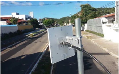
vegetation and medium-sized buildings: this characterizes the environment as suburban (Fig. 1).
The set of equipment used for the transmission and reception of signals comprised a Rhode &
Schwarz broadband amplifier, R&SBBA150 (9 kHz - 6 GHz), and an Anritsu radio transmitter, model
MG3700A (50 Hz - 6 GHz). 15 Watts of power were used to transmit the signal; two pairs of
directive antennas from Pasternack: a panel antenna (2.5 GHz - 2.7 GHz) with a nominal gain of 14
dBi was employed in the 2600 MHz frequency. A panel dual band antenna (806-960MHz and
1710-2500 MHz) with 7 dBi of nominal gain was used in the 800 MHz transmission. The same antennas
were used in the reception of signals. The transmitted signal was a Continuous Wave (CW). The radio
transmitter and the broadband amplifier are showed in Figure 2a.
Fig. 1. One of the streets from Lagoa Nova district, highlighting the panel antenna used in reception.
Regarding the measurement of the signal, an Anritsu spectrum master, model MS2721B (illustrated
in Fig. 2b.), featuring an integrated GPS - responsible for giving the precise location of measured
points, was employed.
The transmitter antenna was installed on the rooftop of the Engineering Technological Complex
(Complexo Tecnológico de Engenharia - ECT) building, in UFRN campus (Figure 3a.), at a height of
20 meters. A high-grade coaxial cable was used to connect the antenna to the broadband amplifier,
which in turn was connected to the digital transmitter.
With the purpose to cover the different points along the site, a mobile laboratory was set - a car,
granted by UFRN, duly equipped with a receiving antenna installed at the top of the vehicle, at a total
height of 3.6 meters, measured from the floor, and connected to the spectrum master. The vehicle
(12.5 mph, approximately).
a) b)
Fig. 2. a) Radio transmitter and broadband amplifier. b) Spectrum master employed in the reception.
a) b)
Fig. 3. a) The mobile laboratory, highlighting the CET building in the background. b)Map containing the routes covered by the campaign [21].
IV. HYBRID ERROR CORRECTION-BASED MODEL
In this research, an error correction-based ANN model, based in [11, 16], using empirical models, is
applied in the prediction of path loss. The ANN is trained to learn the error between measured values
and the ones calculated by the propagation models. The difference error is obtained by:
The two input vectors comprise the distance between the transmitting antenna and the receiving
station, and the difference error, E, for each point. The output vector, also known as the target of the
neural network, comprises the corrected path loss, given by (12):
��
= ��
�− �
(12) The training phase of the neural network structure is represented in Fig.4, while in Figure 5, the
network architecture is depicted.
The implemented ANN is a feedforward Multilayer Perceptron type. Its architecture consists of 2
inputs and 1 output, with 1 hidden layer. The input set consist of two vectors with 455 elements each
(in the 2600 MHz scenario, while in 800 MHz case, it consists in 450 elements).
The transfer functions used for hidden and output layers were the tangent-sigmoid and linear,
respectively, while the algorithm chosen to train the network was the Levenberg-Marquardt
backpropagation [22, 23].
Fig.4. Fluxogram of the training process.
The goal of the path loss prediction is not only produce small errors for the set of the training
examples, but also to be able to present better results dealing with examples not employed in the
training process [11]. This property is called generalization and it is very important to predict path
loss and determine estimated coverage areas properly in different projects within a similar
environment.
A relevant problem that can occur during the ANN training is the over adaptation, or overfitting,
where the network memorizes the training examples and does not learn how to deal with new
Fig.5. Architecture of the designed ANN.
Seeking to avoid overfitting and to make the network to acquire the generalization property, data
was split into three sets (Table II): the first one was used in the training of the network for weights
adjustment. The second set, used as a validation set, checks the efficiency concerning to the network
generalization capability, also serving as a stopping criteria (using a cross-validation strategy [24]).
Meanwhile, the third set, defined as testing set, gives a realistic estimate of the performance of the
learned network on new data.
TABLE II. HYBRID ANN PARAMETERS FROM BASIC CONFIGURATION
Parameter Value Training ratio 60% Validation ratio 25% Testing ratio 15% Max. Number of epochs 1000
Mean Square Error (MSE) was used as performance function by the algorithm to evaluate the
convergence rate. A performance progress plot regarding each set’s curves for ECC model at 2600
MHz is illustrated in Fig.6. There is no indication of any major problems with the process, since the
training, validation, and test curves are very similar. If the test curve had increased before the
validation curve, it would indicate an overfitting problem [14].
The network was designed with a single hidden layer. To find the optimum configuration, a
convergence test was performed, based in a trial-and-error procedure, to select the appropriate number
of hidden nodes for each scenario. The MSE for different numbers of hidden nodes with 5, 10, 20, 30,
and 40 neurons were compared. Each case was executed 30 times, aiming to obtain the average
Fig.6. One of the performances of training, validation, and test sets.
The average MSE for validation set versus the number of hidden nodes for each propagation model
applied are depicted in Table III and Table IV for 800 MHz and 2600 MHz, respectively. Best values
are marked in bold, while the worst outcomes are presented in italic.
TABLE III.MSE OF VALIDATION SET DATA FOR ANNS VERSUS THE NUMBER OF HIDDEN LAYER NEURONS FOR 800MHZ.
Hidden Nodes MSE-Ericson MSE-TR 36.942 MSE- Free Space 5 0.006364931 0.004739687 0.009545273
10 4.173E-06 0.00147253 2.54E-07
20 7.606E-06 0.000517946 0.003228987 30 0.0002562 0.000500116 0.004230354 40 0.0001815 0.001702118 0.00339153
TABLE IV.MSE VERSUS THE NUMBER OF HIDDEN LAYER NEURONS FOR 2600MHZ.
Hidden Nodes MSE-Ericson MSE-TR 36.942 MSE- ECC 5 9.671E-05 0.00665841 0.000473981 10 0.0117833 0.000678807 5.7099E-07 20 4.877E-06 0.000611772 0.027391162
30 0.0077791 0.001425951 0.004246174 40 0.2750327 0.017003488 0.003001516
For the best configuration obtained for each model, we computed the RMSE achieved in the
procedure, also running the neural network another 20 times (50 in total) and computed the value of
RMSE. The results are presented in section V.
A trial-and-error procedure was also conducted to find an efficient configuration for the SNN
model. A configuration with 30 neurons for 800 MHz and 20 neurons for 2600 MHz was then
selected. Data was split using the same proportions as in the HNN model, presented in Table II.
V. ANALYSIS OF RESULTS
The performance of the HNN model, along with the SNN was obtained by comparing RMSE and
approach against data gathered from the measurements. The simulation scenarios were performed for
the operating frequency of 2600 MHz and 800 MHz, transmitted in the campaign.
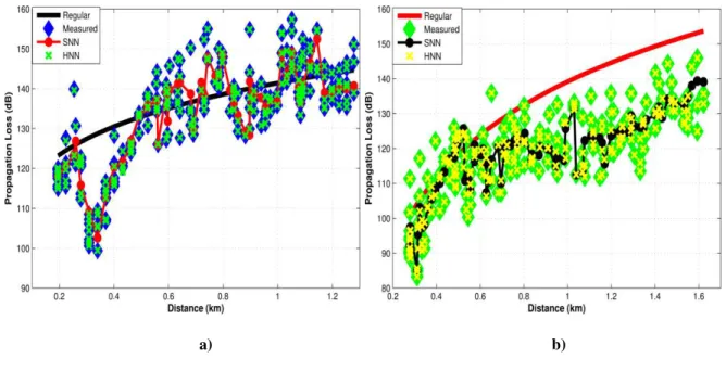
Figure 7 depicts the results for a) ECC model at the frequency of 2600 MHz (route 1), b) Ericsson
model at 800 MHz in route 2 and c) TR 36.942 model at 800 MHz in route 1. In all scenarios, both
ANN-based models showed a well-defined pattern in terms of performance.
The regular variants, although performing satisfactorily, proved to be the less accurate method.
From the beginning of the course of measurements in route 1, up to 500 meters, ECC model
predictions, which obtained a RMSE of 10.33 dB, were positioned far from most measured points.
A less efficient performance can be observed in the regular Ericsson model in route 2, which
achieved 15.58 dB of RMSE, presenting a displacement in relation to measured points from 800
meters until the end of the route. TR 36.942 model presented the best performance among the three
models analyzed, once its path loss curve was located near experimental data along almost the entire
course, obtaining a RMSE of 8.68 dB.
Regarding the SNN model, it obtained a trustworthy performance, following experimental data
closely along the entire course, in all scenarios. This is reflected in the obtained RMSE: the method
obtained 4.61 dB, 5.48 dB, and 4.51 dB for the cases presented in Fig.7.a, Fig.7.b, and Fig.7.c,
respectively.
However, the technique that achieved the highest level of excellence in performance was the hybrid
neural network, once the marks were virtually equal to measured data. The RMSE obtained by the
HNN model was close to 0 dB for all scenarios.
c)
Fig. 7. a)Path loss curves for ECC model at 2600 MHz in route 1. b)Results for Ericsson at 800 MHz in route 2. c)Curves for TR 36.942 model (800 MHz) in route 1.
Fig.8. depicts a box-and-whisker plot with all five datasets from the scenario presented in Fig.7.b.
It can be noted that data distribution from Ericsson model occupied most of the range above the
interquartile range of experimental data, which indicates higher values of propagation loss predicted;
these values deviates from the measurements average, represented by the red line, and only partially
matches with its adjacent quartiles.
Regarding SNN model in this scenario, although slightly flatter, it almost matched the interquartile
range, presenting a high similarity with measured means. However, it obtained decreased data
distribution fidelity, once the span occupied only part of the measured data sampling space. The
hybrid model corrected these issues, obtaining a data distribution as close as it can get to measured
values, reproducing also the outliers, which are represented by the red crosses.
Fig.8. Box-and-whisker plot of Ericsson model in route 2 (800 MHz).
Table V emphasizes the difference in performance between the evaluated methods, considering all
statistical significance level in the experiment. Higher p values indicate that the data distribution is
more similar to the measured values; the threshold for a result to be considered null is any value
below −6. The significance column expresses, based on p value, if the model is considered accurate
and statistically equivalent to actual data. If the p value is below 0.05, the method is considered
Significantly Different (S.D); otherwise, it is classified as Significantly Equivalent (S.E).
TABLE V.RMSE AND P VALUE FOR ALL TECHNIQUES ANALYZED
Route Model RMSE(dB) 800 MHz Wilcoxon rank-sum p-test 800 MHz Significance @95% 800 MHz RMSE(dB) 2600 MHz Wilcoxon rank-sum p-test 2600 MHz Significance @95% 2600 MHz 1
Ericsson 14.9394 0.000316 S.D 10.3154 0.2699 S.E
HNN Ericsson 0.00040766 0.9954 S.E 0.0016907 0.9984 S.E
TR 36.942 8.6792 0.18 S.E 13.0016 0.002567 S.D
HNN TR 36.942 0.00090938 1 S.E 0.000277 0.9860 S.E
Free Space 25.2676 null S.D – – –
HNN Free Space 0.0002416 0.9898 S.E – – –
ECC – – – 9.0942 0.2773 S.E
HNN ECC – – – 0.0015174 0.9727 S.E
SNN 4.5098 0.6871 S.E 4.6107 0.7756 S.E
2
Ericsson 15.5786 0.000123 S.D 10.4004 0.19386 S.E
HNN Ericsson 0.00061889 0.9916 S.E 0.0013104 0.9992 S.E
TR 36.942 7.75 0.0141 S.E 19.0032 null S.D
HNN TR 36.942 0.00073811 0.9978 S.E 0.00026287 0.9959 S.E
Free Space 25.4316 null S.D – – –
HNN Free Space 0.00033739 0.9897 S.E – – –
ECC – – – 10.3305 0.1439 S.E
HNN ECC – – – 0.005393 0.9936 S.E
SNN 5.4864 0.7311 S.E 4.3912 0.6415 S.E
HNN model was able to decrease the RMSE while increasing the p value, rendering the difference
between simulated and measured values to almost zero. This demonstrates the ability of the neural
network to learn and naturally incorporate non-deterministic, uncertain aspects present in the
experimental data.
This feature can also be observed in the SNN approach, which obtained good results in terms of
RMSE and similarity with measurements. Concerning to regular models, Ericsson and ECC models
presented the best results in the 2600 MHz range, while TR 36.942 model stood out for the 800 MHz
frequency range.
VI. CONCLUSIONS
This article proposed a hybrid error-based ANN model using empirical propagation models for the
prediction of path loss in suburban environments. Unlike deterministic and statistical methods,
empirical models require only basic elements present in these models to calculate the path loss.
In order to avoid overfitting and to improve the generalization capability, a cross-validation strategy
along with a test set were performed in the neural network execution. This strategy allows the network
The obtained results were compared against the ones achieved by regular propagation models and a
simple neural network fed with terrain/propagation related inputs. The hybrid error-based model
proved to be more accurate than the other methods in the tested scenarios, presenting the lowest
RMSE indexes and highest p values. The model also performed well when compared with results
obtained by related works, highlighting the difference obtained with respect to [11].
The use of prediction methods through simulation in the planning phase of communication systems
can significantly increase efficiency and precision in diverse radio deployment environments, also
representing the saving of time and money.
Therefore, this new technique is a useful tool for LTE and LTE-A wireless network designers,
proving to be an effective and accurate propagation loss prediction method, as it displayed simulation
data close to actual field measurements. For future works, we intend to expand the scope of the study,
covering new types of terrains, operating frequencies, and propagation models.
ACKNOWLEDGMENT
THE AUTHORS WOULD LIKE TO THANKS THE PPGEEC PROGRAM FROM UFRN(FEDERAL UNIVERSITY OF RIO GRANDE DO NORTE) FOR THE SUPPORT AND ASSISTANCE.
REFERENCES
[1] N. Shabbir et al., “Comparison of Radio Propagation Models for Long Term Evolution (LTE) Network,” International Journal of Next-Generation Networks, vol. 3, no. 3, 2011.
[2] M. Rumney. LTE and the Evolution to 4G: Wireless Design and Measurement Challenges, 2nd ed. United Kingdom: John Wiley & Sons Ltd., 2013.
[3] M. Ahmed, “Performance test of 4G (LTE) networks in Saudi Arabia,” in Proc. International Conference on Technological Advances in Electrical, Electronics and Computer Engineering., Turkey, 2013, pp. 28-33.
[4] N. S. Nkordeh et al., “LTE Network Planning using the Hata-Okumura and the COST-231 Hata Pathloss Models” in World Congress on Engineering., London., UK, 2014.
[5] Y. A. Ahmad et al., “Studying Different Propagation Models for LTE-A System,” in International Conference on Computer and Communication Engineering., Malaysia, 2012, pp. 848–853.
[6] G.R. Pallardó, “On DVB-H Radio Frequency Planning: Adjustment of a Propagation Model Through Measurement Campaign Results,” M.S. thesis, Dept of technology and Built Enviroment, University of Gävle, 2008.
[7] W. Chan, et al., "Listen, attend and spell: A neural network for large vocabulary conversational speech recognition", in Acoustics, Speech and Signal Processing (ICASSP), 2016 IEEE International Conference on. IEEE, 2016. pp. 4960-4964.
[8] T. Wang et al., "A combined adaptive neural network and nonlinear model predictive control for multirate networked industrial process control", in IEEE Transactions on Neural Networks and Learning Systems, v. 27, n. 2, 2016, pp. 416 -425.
[9] W. Li et al., "Deepreid: Deep filter pairing neural network for person re-identification", in Proceedings of the IEEE Conference on Computer Vision and Pattern Recognition, 2014. pp. 152-159.
[10] F.G. Aguia, “Utilização de redes neurais artificais para detecção de padrões de vazamento em dutos,” Ph.D. dissertation in portuguese, Federal University of São Paulo., São Carlos., SP, 2010.
[11] I. Popescu et al., “Comparison of neural network models for path loss prediction,” in IEEE International Conference on Wireless And Mobile Computing, Networking And Communications., Montreal., QC, 2005, pp. 44–49.
[12] D. Wu et al., “Application of artificial neural networks for path loss prediction in railway environments”, in Communications and Networking in China, 2010, pp. 1-5.
[13] E. Ostlin et al.,"Macrocell radio wave propagation prediction using an artificial neural network", in Vehicular Technology Conference, 2004. VTC2004-Fall. 2004 IEEE 60th vol.1, 2004, pp. 57-61.
[14] E. Ostlin et al., "Macrocell path-loss prediction using artificial neural networks", in IEEE Transactions on Vehicular Technology, v. 59, n. 6, 2010, pp. 2735-2747.
[15] C. D. Angeles and E. P. Dadios., “Neural network-based path loss prediction for digital TV macrocells,” in Humanoid, Nanotechnology, Information Technology, Communication and Control, Environment and Management., Cebu., PH, 2015.
[16] I. Popescu et al., “Applications of generalized RBF-NN for path loss prediction,” Personal, Indoor and Mobile Radio Communications, 2002. The 13th IEEE International Symposium on, vol. 1, 2002, pp. 484-488.
[17] S. S. Kale and A. N. Jadhav, “Performance analysis of empirical propagation models for WiMAX in urban environment,” OSR J. Electron. Commun. Engin, 2013.
[18] LTE; Evolved Universal Terrestrial Radio Access (E-UTRA); Physical channels and modulation (3GPP TS 36.211 version 8.7.0 Release 8), ETSI, 2009.
[19] J. Milanovic et al., “Comparison of propagation model accuracy for WiMAX on 3.5GHz” in 14th IEEE International conference on electronic circuits and systems., Marrakech., MA, 2007.
[21] Google Maps, 2016. Map of UFRN campus. [online]. Google. Available from: https://goo.gl/maps/1RbPQwn5o6y [Accessed 24 November 2016].
[22] D. Marquardt, “An Algorithm for Least-squares Estimation of Nonlinear Parameters,” SIAM Journal Applied Mathematics, vol. 11, 1963, pp. 431–441.
[23] J. J. Moré, “The Levenberg-Marquardt Algorithm: Implementation and Theory,” Numerical Analysis, ed. G. A. Watson, Lecture Notes in Mathematics 630, Berlin: Springer Verlag, 1977.
![Fig. 3. a) The mobile laboratory, highlighting the CET building in the background. b) Map containing the routes covered by the campaign [21]](https://thumb-eu.123doks.com/thumbv2/123dok_br/18888295.424364/7.893.108.785.476.901/mobile-laboratory-highlighting-building-background-containing-covered-campaign.webp)