Programa de P´os-Graduac¸˜ao em F´ısica - PPGFis Departamento de F´ısica
Flux avalanches in patterned superconducting thin
films: ac susceptibility, morphology and related
studies
Avalanches de fluxo em filmes finos supercondutores estruturados:
suscetibilidade ac, morfologia e outros estudos
Maycon Motta
Flux avalanches in patterned superconducting thin
films: ac susceptibility, morphology and related
studies
Avalanches de fluxo em filmes finos supercondutores estruturados:
suscetibilidade ac, morfologia e outros estudos
Tese apresentada ao Programa de
P´os-Gradua¸c˜ao em F´ısica da Universidade Federal de S˜ao Carlos como parte dos requisitos
para a obten¸c˜ao do T´ıtulo de Doutor em
Ciˆencias com ˆenfase em F´ısica.
Advisor (Orientador):
Prof. Dr. Wilson Aires Ortiz
Co-Advisor (Co-orientador):
Prof. Dr. Alejandro Vladimiro Silhanek
Ficha catalográfica elaborada pelo DePT da Biblioteca Comunitária/UFSCar
M921af
Motta, Maycon.
Avalanches de fluxo em filmes finos supercondutores estruturados : suscetibilidade ac, morfologia e outros estudos / Maycon Motta. -- São Carlos : UFSCar, 2013. 148 p.
Tese (Doutorado) -- Universidade Federal de São Carlos, 2013.
1. Supercondutividade. 2. Flux jumps. 3. Instabilidades termomagnéticas. 4. Filmes finos. I. Título.
Acknowledgements (Agradecimentos)
No fim de um trabalho de doutorado, h´a muitas pessoas para agradecer, que de alguma forma ajudaram nessa longa jornada. Primeiramente, minha fam´ılia que conta com um integrante rec´em-chegado, Vict´orio. Em especial, `a Tati por estar sempre ao meu lado. Pela sua paciˆencia, apoio e por entender minha ausˆencia. `A minha m˜ae pela preocupa¸c˜ao e apoio. `A Fabi, minha irm˜a, que est´a conseguindo ultrapassar um momento delicado de sua vida. Ao Rog´erio, meu cunhado, pela for¸ca. `A minha sogra, Stella, pelo apoio. `A Dona Maria Diagonel e fam´ılia pela sabedoria, carinho e amizade ao longo desses anos. Mesmo h´a algum tempo separados, ao meu falecido avˆo, Vict´orio, cujo incentivo foi crucial no in´ıcio da minha vida cient´ıfica. Nos momentos dif´ıceis o apoio e o incentivo de vocˆes me ajudaram muito.
Ao Prof. Ortiz por acreditar que poderia fazer um bom trabalho. Pelo incentivo quando tudo parecia complicado. Por estar sempre pronto para longas discuss˜oes, muitas vezes at´e altas horas, sobre medidas, resultados e ciˆencia em geral. Por fim, por mostrar via exemplo que ´e importante se dedicar e se preocupar com a forma¸c˜ao do estudante.
I am very grateful to Alejandro V. Silhanek, who kindly allowed me to work with him in Leuven. For teaching me a lot about structured superconductors. Also for helping me in some hard moments. Thanks a lot!
Ao Prof. Fabiano Colauto, pelas discuss˜oes que levaram a construir este trabalho. Al´em disso, pela imprescind´ıvel habilidade com as esta¸c˜oes experimentais do GSM, principalmente a de Imageamento por Magneto-´otica.
Tamb´em ao Prof. Dr. Paulo Noronha Lisboa Filho pelo incentivo nos anos de gradua¸c˜ao, mestrado e tamb´em no doutorado. Ao Zad (Prof. Rafael Zadorosny) pelas discuss˜oes no in´ıcio do trabalho e tamb´em pela amizade ao longo desses anos.
Agrade¸co profundamente aos amigos e colegas do Grupo de Supercondutividade e Magnetismo: Alexandre J. Gualdi (algoritimo do C´esar), Andr´e Varella (´E melhor n˜ao dizer nada! Shhhh...), C´esar V. Deimling (Zinguem danguem zinguem!), Cl´audio (“Waldem´a!”), Danusa (Danuzz´on!), Driele (ah Dona Dri!), Fernanda (ah DONA Fernanda!), Korllvary (e o lagarto do RU!), Leonardo (sempre bem humorado), Marlon (Pisco!), Jerˆe (Ricardo!) e Pedro Schio (CGS ou SI!? E o vidraceiro?!). Tamb´em aos amigos Rafael R. G. Paranhos (Joe!) e Adriano V. de Carvalho (Z´e fofinho!).
INPAC, KU Leuven (Leuven, Belgium). I want to express my gratitude to Jo Cuppens, Weldeslassie Ataklti, Denitza Denkova, and Dorin Cerbu for helping me in the lab and also outside it. Thank you all for the experience that I had in Leuven! I would also like to thank Jørn Inge Vestg˚arden for the simulations using the thermomagnetic model presented in Chapter 8 and for the interesting discussions.
`
aprendermos a ter coragem. Isso mesmo! Ser pai ou m˜ae ´e o maior ato de coragem que algu´em
pode ter, porque ´e se expor a todo tipo de dor, principalmente da incerteza de estar agindo
corretamente e do medo de perder algo t˜ao amado. Perder? Como?
N˜ao ´e nosso, recordam-se? Foi apenas um empr´estimo!
Abstract
Avalanches are sudden dramatic phenomena that occur in nature. The technique of magneto-optical imaging (MOI) has allowed us to observe abrupt flux entrances in superconductors, the so-called flux avalanches, due to thermomagnetic instabilities in the vortex matter. Their morphology is fascinating, especially in superconducting thin films, where they develop in dendritic patterns. From a practical point of view, the flux avalanches undermine applications of superconducting thin films. In the last years, however, several steps have been reached to fully understand the fundamental physics of the phenomenon and also on how to suppress their occurrence.
The present thesis deals with the study of flux avalanches in structured superconducting thin films. We have studied crystalline Nb and amorphous Mo79Ge21
thin films decorated with arrays of antidots (ADs or holes) produced by electron beam lithography. The magnetic response of these specimens has been investigated by means of MOI, dc magnetization and ac susceptibility. Firstly, we have established a link among those three techniques in the regime dominated by flux avalanches. We have observed that the reentrant behavior in the ac susceptibility at low temperatures occurs as a consequence of flux avalanches. Essentially, there is reuse of the channels created by the first ac cycle in a regime where the signal is weakly dependent on the temperature. Our results show that measurements of ac susceptibility versus ac field amplitude can be used to detect flux avalanches, since the signature of the flux avalanches appears as noisy curves of both ac susceptibility components. As a consequence, the critical current density as a function of temperature [JcT] obtained by using the Bean model – whose
validity is assured by Cole-Cole plots – is smooth for higher temperatures and, below a certain temperature onset, a non-smooth and noisy behavior takes place due to the avalanches. The temperature dependence of JcT, H was determined for different
values of the applied magnetic field. The stability/instability frontier was then identified as the limiting temperature below which the curve JcT, H becomes noisy, indicating
the occurrence of avalanches. Associated with this limiting temperature, the threshold critical current density to trigger avalanches is essentially independent of the magnetic field. This frontier corresponds to the upper threshold limit for the occurrence of avalanches.
the flux avalanches, highly induced by the presence of an array of ADs, have their activity reduced in temperature and magnetic field. For the first time, flux avalanches have been visualized in amorphous Mo79Ge21 thin film, both in plain and decorated thin films.
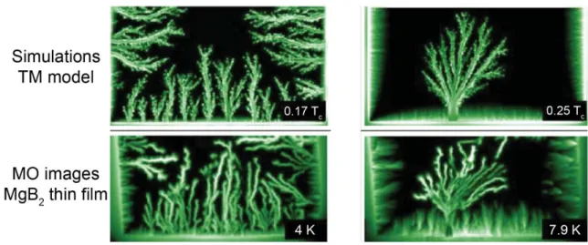
Finally, we have investigated the influence of the lattice symmetry and AD geometry on the flux avalanche morphology. We have observed avalanches with the habit of forming trees where the trunk is parallel to the main axis of the square lattice and the branches form angles of 45 degrees. In addition to that, we have found an anisotropic penetration in a Nb thin film decorated with a square lattice of triangular ADs. Besides that, a sample having one half of the ADs in the form of squares, and the other half being circles, has been observed to present avalanches of different morphologies on each of its halves. We have also studied an a-MoGe thin film with a centered rectangular 2D Bravais lattice with square ADs which shows penetrations with different angles depending on the edge. The overall features of the avalanches, and in particular the 45-degree direction of the branches, have been confirmed by numerical simulations using the thermomagnetic model.
Resumo
Avalanches s˜ao eventos repentinos e dram´aticos que ocorrem na natureza. A t´ecnica de imageamento por magneto-´otica (MOI) tem permitido visualizar a penetra¸c˜ao abrupta de fluxo em supercondutores, as chamadas avalanches de fluxo, que ocorrem devido a instabilidades termomagn´eticas na mat´eria de v´ortices. A morfologia dessas avalanches de fluxo em filmes finos supercondutores pr´ıstinos ´e singular e se desenvolve de maneira dendr´ıtica, isto ´e, com ramifica¸c˜oes. Do ponto de vista pr´atico, as avalanches de fluxo s˜ao prejudiciais para aplica¸c˜oes dos filmes finos supercondutores. Nos ´ultimos anos, no entanto, tem-se alcan¸cado um bom entendimento da f´ısica b´asica do fenˆomeno, bem como maneiras para suprimir essas avalanches.
Esta tese trata do estudo de avalanches de fluxo em filmes finos com uma estrutura de defeitos. Para tal, usamos filmes finos cristalinos de Nb e amorfos da liga Mo79Ge21
decorados com arranjos de antidots (ADs), ou buracos, produzidos por litografia por feixe de el´etrons. A resposta magn´etica desses filmes foi investigada atrav´es de MOI, magnetiza¸c˜ao dc e suscetibilidade ac. Na primeira parte dos resultados, uma conex˜ao entre essas t´ecnicas foi estabelecida no regime de avalanches de fluxo. Foi observado que o comportamento reentrante da suscetibilidade ac em baixas temperaturas ocorre devido `as avalanches de fluxo. Essencialmente, h´a o reuso dos caminhos ou canais criados pelo primeiro ciclo ac em um regime em que o sinal ´e fracamente dependente da temperatura. Esses resultados tamb´em mostraram que a suscetibilidade ac pode ser usada para detectar avalanches de fluxo, seja pela constru¸c˜ao da curva de corrente cr´ıtica dependente da temperaturaJcTou monitorando o ru´ıdo nas curvas do tipo Cole-Cole.
Assim, a fronteira de instabilidades termomagn´eticas/estabilidade foi constru´ıda variando-se o campo dc aplicado, tendo sido obtido, um limiar constante de JcT para
o disparo das avalanches. Essa observa¸c˜ao est´a de acordo com o modelo termomagn´etico e refere-se ao limite superior da ocorrˆencia das avalanches de fluxo.
Por fim, a influˆencia da simetria da rede e da geometria do antidot na morfologia das avalanches de fluxo foi investigada. Para filmes finos decorados com uma rede quadrada de ADs quadrados, as avalanches tˆem o tronco paralelo ao eixo principal da rede de ADs, com ramifica¸c˜oes em ˆangulos de 45 graus como em uma ´arvore de Natal. Al´em disso, penetra¸c˜oes abruptas anisotr´opicas foram vistas em um filme fino de Nb decorado com uma rede quadrada de ADs triangulares. Uma mudan¸ca na morfologia das avalanches tamb´em foi observada em um filme com metade dos ADs quadrados e a outra metade circular. Tamb´em foram observadas penetra¸c˜oes com diferentes ˆangulos em uma rede retangular centrada de ADs quadrados dependendo da borda. Por fim, as caracter´ısticas gerais das avalanches, em particular a de ramifica¸c˜oes em 45 graus, foram confirmadas por simula¸c˜oes num´ericas usando o modelo termomagn´etico.
Contents
Acknowledgements (Agradecimentos) . . . iv
Abstract . . . vii
Resumo . . . ix
1 Overview 1 2 Basic aspects of superconductivity 5 2.1 Superconductivity: basic concepts and historical notes . . . 5
2.2 London model . . . 6
2.3 Ginzburg-Landau theory . . . 8
2.3.1 Clean and dirty limits of λ and ξ . . . 11
2.4 Type I and Type II superconductors . . . 12
2.5 Flux quantization, vortex structure, and the Abrikosov lattice . . . 15
2.6 Real superconductors: the pinning centers . . . 19
2.6.1 Intrinsic pinning . . . 20
2.6.2 Artificial pinning . . . 21
2.7 Critical state models: the Bean model . . . 23
2.7.1 Slab/cylinder: parallel configuration . . . 25
2.7.2 Thin film: perpendicular configuration . . . 26
3 Flux avalanches in superconductors 31 3.1 Introduction . . . 31
3.2 Thermally driven avalanches: flux avalanches . . . 32
3.2.2 The thermomagnetic model . . . 37
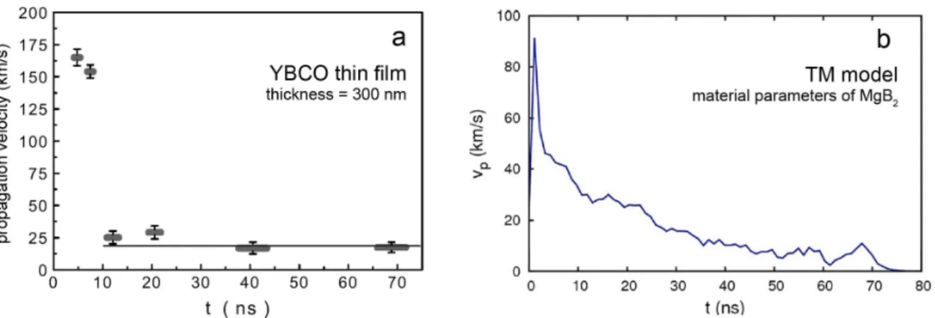
3.3 Dynamic properties of the flux avalanches . . . 39
3.4 Avoiding flux avalanches . . . 44
4 Experimental techniques 47 4.1 Sample preparation . . . 47
4.1.1 Electron beam lithography . . . 47
4.1.2 Pulsed laser deposition . . . 49
4.1.3 Dc-magnetron sputtering . . . 51
4.2 Sample characterization . . . 51
4.2.1 Structural characterizations based on X-ray . . . 52
4.2.2 Atomic force microscopy . . . 53
4.2.3 Scanning electron microscopy . . . 53
4.3 Magnetic measurements . . . 54
4.3.1 Magneto-optical imaging . . . 54
4.3.1.1 MOI workstation at GSM/S˜ao Carlos . . . 57
4.3.2 SQUID: dc measurements . . . 59
4.3.3 PPMS: ac measurements . . . 62
4.3.3.1 Ac susceptibility details and Cole-Cole curves . . . 64
5 Visualizing ac susceptibility and ac field effects on flux avalanches 69 5.1 Introduction . . . 69
5.2 Samples and experimental techniques . . . 70
5.3 Results and discussion . . . 72
5.4 Conclusions . . . 81
6 Threshold of critical current densities to trigger flux avalanches in
6.1 Introduction . . . 82
6.2 Instability region in superconducting thin films . . . 84
6.3 Experimental details . . . 86
6.4 Results and discussions . . . 86
6.5 Conclusions . . . 91
7 Enhancement of pinning properties of superconducting thin films by graded pinning landscapes 92 7.1 Introduction . . . 92
7.2 Experimental details . . . 94
7.3 Results and discussions . . . 95
7.4 Conclusions . . . 98
8 Guidance and morphology of flux avalanches in superconducting films decorated with lattices of antidots 99 8.1 Introduction . . . 99
8.2 Samples and experimental techniques . . . 101
8.3 Results and discussions . . . 102
8.4 Conclusions . . . 110
9 Conclusions and perspectives 111 Appendix A -- Shape and profile studies of antidots in decorated thin films113 Appendix B -- Current crowding effects in superconducting corner-shaped Al microstrips 117 B.1 Introduction . . . 117
B.2 Samples and experimental techniques . . . 119
B.3 Results and discussion . . . 119
List of Publications 125
1
Overview
Superconductivity is an important area in Condensed Matter Physics. Its mechanisms are not completely understood yet for all superconducting materials, in spite of its discovery more than 100 years ago. Since then, five Nobel prizes in topics directly related to superconductivity have been awarded: Heike Kamerlingh Onnes in 1913, for his studies on the matter in low temperatures; John Bardeen, Leon Neil Cooper, and John Robert Schrieffer (1972) for the microscopic theory of superconductivity; Brian David Josephson, Leo Esaki, and Ivar Giaever because of their studies in tunneling in semiconductors and superconductors (1973); Johannes Georg Bednorz and Karl Alexander M¨uller for the discovery of High Temperature Superconductors (1987); and Alexei Alexeevich Abrikosov, Vitaly Lazarevich Ginzburg, and Anthony James Leggett in 2003 for their pioneering contributions to the theory of superconductors and superfluids [1].
The work of the last Nobel Prize laureates were especially important for describing the behavior of superconductors immersed in a magnetic field. Abrikosov [2], using the theory developed by Ginzburg and Landau [3], found that the magnetic field penetrates into the so-called type II superconductors as quantized units of flux, forming the mixed state. In pure superconducting materials, these entities organize themselves in a regular hexagonal lattice. However, defects commonly present in real materials act as pinning centers, creating an attractive potential for the vortices inside the superconductors and destroying the long-range order. The termVortex Matterwas coined to refer to the vortex system residing in the mixed state of a type II superconductor, which can be organized in different states of aggregation: solid, liquid, and glassy. After the discovery of the High Temperature Superconductors (HTS) in 1986 [4], the liquid and glassy phases have effectively entered the scene, since thermal energies involved made possible the melting of the vortex solid below the critical temperature.
of view, the importance of detecting and understanding magnetic flux avalanches lies in the fact that it modifies the current-carrying capability of the specimen. Then, it might undermine potential technological applications, such as, for example, superconducting fault current limiters, as pointed out in a Technical Report entitled Basic research needs for superconductivity [5] published in 2006 by the U. S. Department of Energy.
This thesis is a natural continuation of some of the last doctorate studies developed at theGrupo de Supercondutividade e Magnetismo(GSM) inUniversidade Federal de S˜ao Carlos (UFSCar). Fabiano Colauto [6] made the first investigations on flux avalanches in plain films, as well as the magnetic braking effect of a metal foil on top of them. Besides that he has assembled the magneto-optical imaging setup in the group; Rafael Zadorosny [7] studied the vortex dynamics in decorated thin films, firstly nanoindentated ones and after lithographically patterned with antidots; Ana Augusta M. de Oliveira [8] investigated in depth systems with controlled defects by using the third harmonics of the complex ac susceptibility. Besides those influences above described, the period that I spent in Leuven has also been significant to the development of the present work, because of the exposure to different kinds of techniques and problems.
The aim of this thesis is to clarify the occurrence and the morphology of flux avalanches in superconducting thin films of crystalline Nb and amorphous Mo79Ge21,
with and without an antidot array prepared by electron beam lithography, by means of MOI, dc magnetization and ac susceptibility measurements. We have investigated the signature of the flux avalanches in ac susceptibility and the threshold for its occurrence, showing that the thermomagnetic model picture is perfectly adequate to describe the results. The effects of a graded distribution of antidots on the critical current density and on the occurrence of flux avalanches were also traced, as well as the effects of antidot geometry and lattice symmetry on the morphology of flux avalanches. This thesis is organized as follows:
The theoretical framework for superconductivity is addressed in Chapter 2. It is shown in details the London model and the Ginzburg-Landau theory, as well as the existence of type I and type II superconductors, the flux quantization, the vortex structure and the Abrikosov lattice. The presence of pinning centers in the superconductor is treated, as well as the consequences of introducing artificial pinning centers for the superconducting properties. In the end, the Critical State Models and the effect of thin film geometry on the Bean critical state model are discussed.
summarizes the dynamical development of the vortex landscape in the Bean model by non-destructive vortex avalanches. Nonetheless, the current understanding of the flux avalanches treated in this thesis is based on the occurrence of thermomagnetic instabilities in the superconductors which are explained by the existence of a positive feedback: flux movement heat generation locally temperature increase pinning force decrease more flux movement etc. The chapter is devoted to thorough discussion of the thermomagnetic model, including some important theoretical and experimental results relating to this intriguing phenomenon.
Chapter 4 contains the details of preparation techniques used to fabricate the array of antidots and the deposition techniques as well. The structural characterization of the thin films is also described in this chapter. The measurement platforms PPMS and MPMS are thoroughly described as well the ac susceptibility technique. The evolution of the Faraday-active crystal used to reveal the flux distribution is reviewed and the MOI workstation at GSM/S˜ao Carlos is described in detail.
The first results are reported in Chapter 5. MO images were used to prove that the reentrance in ac susceptibility versus temperature measurements is really linked to the occurrence of flux avalanches. We also show the correspondence between MOI, dc magnetization and ac susceptibility to recognize the existence of these abrupt events. An alternative way of determining the threshold critical current density (Jcth) to trigger flux
avalanches is discussed in Chapter 6. The existence of Jcth is demonstrated by means of
the thermomagnetic model and the frontier of where the avalanches take place, HthJ c,
was determined.
Chapter 7 deals with a comparative analysis among a plain a-Mo79Ge21 film, a
second film with a uniformly distributed array of antidots, and a thin film with a graded distribution of antidots. The results have shown that the graded array increases the critical current density and decreases the avalanche activity in comparison with the corresponding results for a uniform array. Moreover, we report the first observation of flux avalanches in a plain a-Mo79Ge21 thin film.
An investigation of the flux avalanche morphology is presented in Chapter 8. The influence of different antidot lattice symmetries and AD geometries on the branching was traced. In thin films of crystalline Nb and a-Mo79Ge21 decorated with a square lattice
that, a film decorated with a square lattice of triangular ADs have shown anisotropic penetration, depending on the direction relative to the triangle, i.e., if the flux enters facing a tip or an edge of the AD. Branching with 90 degrees appear in a film with a square lattice of circular ADs, whereas in a film with a centered rectangular lattice of square ADs the avalanche morphology is clearly defined by the lattice geometry. In order to explain such branching of the flux avalanches, we have used the idea published in a very recent paper by us, for L-shaped microbridges, where flux penetrates easier into the inner concave angle, due to a crowding effect on the currents. This work is presented as an appendix (Appendix B) to the thesis. Moreover, Appendix A shows an investigation, using AFM and SEM, of the spatial quality of the ADs of the decorated thin films studied here. The Nb film with ADs of 0.4 µm and lattice parameter of 1.5 µm, presented in Chapter 5, has rounded ADs, whereas the a-MoGe thin film with the same AD size and lattice parameter, presented in Chapter 8, has sharp square ADs being this the reason the different avalanche morphologies.
2
Basic aspects of
superconductivity
This chapter deals with the main characteristics of superconductivity, the phenomenological theories and their implications, such as the discovery of the basic lengths, penetration depth and coherence length, defining the type of superconducting material, the penetration of the magnetic field in the case of type II superconductors, in form of flux vortices, and how theses vortices are distributed throughout the material. In the end, the impact of thin film geometry on the magnetic response will be treated...
2.1
Superconductivity: basic concepts and historical
notes
At the beginning of the 20th century science underwent an enormous and deep
development, especially Physics. The introduction of new ideas and concepts associated with the quantum mechanics led to breakthroughs, resulting in several advances in the comprehension of properties of the matter. In this context, the physicist Heike Kamerling Onnes, who worked in Leiden (The Netherlands) with cryogenic systems, liquefied helium in 1908, allowing him to reach temperatures as low as 4.2 K and thus marked a new chapter in history of low temperature physics. Once this was achieved, the next step was developing controlling apparatus which provided essential tools to study materials at low temperatures. Three years later, in 1911, he and his team were exploring the influence of impurities on the electrical resistance of metals at low temperatures [9], and they observed that the resistivity of pure mercury dropped suddenly more than four orders of magnitude in a narrow temperature range around 4.2 K, which was called the critical temperature (Tc). This property (perfect conductivity)
was recognized as being of great significance for applications, such as coils to generate high magnetic fields [10]. Moreover, another striking signature of the superconducting materials was observed by Walter Meissner and Robert Ochsenfeld in 1933 [11, 12]. They found out that lead and tin cylinders, immersed in an external field, expelled the magnetic flux below their Tc of 7.2 K and 3.7 K, respectively, independent of their
field or vice-versa. This effect was called perfect diamagnetism or Meissner-Ochsenfeld effect, but nowadays called only Meissner effect, and could not be explained only considering perfect conductivity, since a hypothetical perfect conductor would not exclude magnetic flux from its interior decreasing the temperature below Tc under an
applied field. Thereby, the perfect conductivity and the perfect diamagnetism are two independent and intrinsic features of the superconducting state.
In order to fully understand this phenomenon, the perfect diamagnetism was firstly treated by the London brothers [13], in 1935. Later on, in 1950, V. Ginzburg and L. Landau [3] applied the phase transition theory for the superconducting state and obtained a more complete description of it. Both theories are phenomenological ones and will be treated in details in the following sections using SI units. Nonetheless, the microscopic nature of the superconductivity was proposed by J. Bardeen, L. Cooper and J. Schrieffer in 1957 [14], known as BCS theory. The main idea is the presence of an attractive interaction between two electrons, forming the so-called Cooper pairs, which should have opposite momenta and opposite spins. This attractive interaction is intermediated by the lattice vibrations (phonons) and became evident by means of the discovery of the isotope effect in mercury [15, 16], where the critical temperature of the isotopes is proportional to ºM, where M represents the mass of the isotope. Although the BCS theory describes the mechanism for superconducting metals, some alloys, intermetallic compounds, and ionic compounds, it does not describe the mechanism for the High Temperature Superconductors (HTS), discovered in 1986 [4], and for other unconventional superconductors such as heavy fermions, organics and iron-based compounds [17, 18, 19]. The HTS materials are ceramics, with Cu-O planes in their crystallographic structures, and exhibit superconductivity above the limit of approximately 30 K implied by the BCS theory. For example, the mechanisms of superconductivity in YBCO (YBa2Cu3O7δ) [20], which was the first superconducting
material to exceed the boiling point of liquid nitrogen (77 K), with Tc = 92 K cannot be
accounted for by the BCS theory. In fact, this theory provides a microscopic explanation for the mechanism in some superconducting materials, but a complete description, including the unconventional superconductors, still lacks in the literature.
2.2
London model
reported two years earlier. This description was based on the two-fluid model for superconductivity, proposed by Gorter and Casimir [21], in which the average number of conduction electrons per unit of volume, nt, is composed by the sum of two temperature
dependent contributions for T @ Tc: a normal fluid (nnT) and a superfluid (nsT).
The normal fraction nnT is associated to the density of normal electrons, behaving as
in a viscous medium, whereas the superfluidic portionnsT is related to the density of
electrons which experience no scattering and are responsible for the impressive properties of the superconductors, called superconducting electrons or superelectrons. When T Tc, ns tends to zero and at T 0 K, all the electrons are taking part in the
superconducting state. Applying the equation of motion to the portion ns, as the Drude
model for electrical conductivity in a metal [22], it leads to the first London equation, in SI units:
E m
nse2
∂Js
∂t (2.1)
where E is the electric field, m and e are the effective mass and charge of the superelectrons and Js is the superconducting current density, which is given by:
Js nsevs (2.2)
where ns and vs are the density and the velocity of the superelectrons. As described by
the BCS theory, the superelectrons are composed by electron pairs – or Cooper pairs – and, thus,m 2me and e 2e, with me and e the mass and the charge of the electron,
respectively. Eq. (2.1) shows that in the superconducting steady state, the electric field is null, i.e., the voltage across the superconductor is zero (infinite conductivity) and the superconducting current is constant. In order to obtain the second London equation, which enables one to calculate the local field inside the superconductor, one combines Eq. (2.1) and the Maxwell equations to obtain:
∂
∂t© © B
µ0nse2
m B 0 (2.3)
whereB is the magnetic induction and µ0 is the magnetic permeability of vacuum.
This equation, however, is not compatible with the Meissner effect, since the magnetic field could not change temporally (∂B
∂t © E 0). Thus, the London
brothers restricted the solutions to those that follow the condition
© © B µ0nse
2
m B, which leads to the Meissner effect. Therefore, the second London
equation is obtained as:
λ2
or
©2
B 1
λ2
L
B (2.5)
where λL
¼
m µ0nse
2 is known as the London penetration depth and it is one of the
fundamental lengths of superconductivity. Besides the trivial solution B = 0, the only possible solution for a semi-infinite superconductor in the region x A0 occurs when B
vanishes exponentially in the interior of a superconducting bulk, and λL provides the
characteristic distance along which the field decays from its value at the surface in the Meissner state, where B = 0 [17]. Indeed, the superconducting current can be written as:
©2
Js 1
λ2
L
Js (2.6)
The expression above means that the currents responsible for the Meissner effect are superficial currents, also called shielding currents, which circulate over the distance λL
into the superconducting bulk. This shielding currents are responsible for the null induction field (B = 0) inside the superconductor. It means that the current generates a magnetization equals to the opposite of the field strength (M = –H).
The London approach assumes that the density of Cooper pairs nsT is constant
along the whole superconductor, as a consequence of its local character, where the fields and currents are determined at the point r. When non-local characteristics are taken into account, i.e., Jsr depends on the magnetic vector potential, A, around the considered point r, as showed by A. B. Pippard [23], the second fundamental length of the superconductivity emerges, known as coherence length, which will be discussed within the scope of the Ginzburg-Landau (GL) theory.
2.3
Ginzburg-Landau theory
In 1950, V. L. Ginzburg and L. D. Landau proposed their theory for superconductivity [3] based on the Landau theory for second-order phase transitions developed earlier [24]. In zero magnetic field, the transition from the normal to the superconducting state is a second-order phase transition, experimentally supported by the discontinuity on the specific heat at T Tc [17]. The main idea of the Landau theory
is the existence of an order parameter to describe a transition from a disordered to an ordered phase [25]. For the case of a superconductor, a complex order parameter, ψr,
is defined as:
ψr SψrSeiϕr
(2.7) where φr is a phase factor. This order parameter is employed to describe the phase transition, being null aboveTc and nonzero below Tc. Physically, the order parameter is
related to the density of superconducting electronsns, as following:
ns SψS
2
(2.8)
According to the phase transition theory, the free energy is real and should reach a minimum value. As a consequence, it can be expanded in series of SψS2 for temperatures near Tc and terms of order larger than two (in this case SψS
4
) can be neglected. The Gibbs free energy per unit volumeGs in the superconducting state, in the presence of an
external field, is then:
Gs GnαT SψS
2
β
2SψS
4
1
2mSiÒh© e
AψS2
B
2
2µ0
(2.9)
whereGnis the free energy density of the normal state,hÒ is the Planck constanthdivided
by 2π, αT and β are phenomenological parameters of the expansion. The second and third terms on the right side of the equation are related to the expansion, the fourth represents the kinetic energy of the superelectrons, and the fifth refers to the energy density due to the magnetic field. Minimizing the free energy with respect to SψS2 and with respect toA leads to two coupled differential equations, named as the first and the second Ginzburg-Landau equations, respectively:
αψβSψS2ψ 1
2mihÒ© e
A2
ψ 0 (2.10)
Js iehÒ
2m ψ
©ψψ©ψ e2
m SψS
2
A e
2
mSψS
2
hÒ
e©ϕA (2.11)
βA0.
It is possible to determine the second fundamental length of superconductivity from a condition similar to that described above. Considering a boundary condition of being near the surface, for a semi-infinite superconductor at xA0 in the absence of field, Eq. (2.10) can be written by means of a new function f, defined as f ψ~ψª. In this case, one has
Ò
h2
2mSαTS©
2
ff1f2 0 (2.12) where
ξ2 Òh
2
2mSαTS
1 1TT
c
(2.13) has a square length dimension. Thus, the order parameter ψ for x 0 is obtained as being:
ψx ψªtanhºx
2ξ (2.14)
Therefore, ξ determines the scale of distances for spatial variations of the order parameter ψ, called the coherence length. It defines the typical size of the Cooper pairs, i.e., the minimum length within which the number of superelectrons varies significantly [2].
The penetration depthλLcan also be obtained through the GL theory. In a weak field,
the order parameter remains almost constant and can be substituted byψª in Eq. (2.11),
Js e
2
mSψªS
2
A 1
µ0λ 2
L
A (2.15)
By applying © Js and the Maxwell equation © B µ0J, one has:
©2
B µ0e
2Sψ
ªS
2
m B (2.16)
which is similar to the second London equation (Eq. (2.5)) written in other terms, where the penetration length equals to
λ2
L
mβ µ0e2SαTS
1
1 T Tc
(2.17)
Thus, the penetration depth and the coherence length can be obtained from the GL theory, as well as their temperature dependences close toTc. The temperature range is the
main limitation of this theory, since it is valid only forT Tc. Although the GL theory is
of the microscopic theory, suitable to T near Tc. However, it is also a powerful theory,
since it describes the two forms of behavior of the superconductors in the presence of a magnetic field, the flux quantization, the characteristics of the vortex and its interactions in the mixed state.
2.3.1
Clean and dirty limits of
λ
and
ξ
Since the London penetration depth and the coherence length have been described by the GL theory, it is important to take into account the presence of impurities (and defects) and their influence on these lengths [27, 28]. Depending on themean free path le
of the electron and theBCS coherence length ξ0 introduced by the BCS theory, given by:
ξ0 0.18
Ò
hvF
kBTc
(2.18) where kB is the Boltzmann constant andvF is the Fermi velocity (106 m/s in metals),
there are two limiting cases: (i) the clean limit when le Qξ0, generally for pure metals,
and (ii) thedirty limit when lePξ0, for alloys and metals with defects and impurities.
In the dirty limit, the penetration depth [λT] and the coherence length [ξT] are
ξT 0.855»ξ0le1
T Tc
1
2
(2.19)
λT 0.64λL0
¾
ξ0
le
1 T
Tc
1
2
(2.20) whereλL0 is the penetration depth obtained by the London theory atT = 0 K. In the
clean limit, they are:
ξT 0.74ξ01
T Tc 1 2 (2.21)
λT 0.71λL0 1
T Tc
1
2
(2.22)
An important consequence of the GL theory is the Ginzburg-Landau parameter κ
defined as:
κ λT
ξT (2.23)
2.4
Type I and Type II superconductors
The superconducting materials can be distinguished into two kinds, type I and type II, depending on their behavior in the presence of an applied field. Considering a normal-superconductor interface and neglecting any demagnetization effect, the surface energy (σns) given by the difference between the Gibbs free energy per unit area of a homogeneous
phase (normal or superconducting) and a mixed phase (region where the superconductivity is not completely established, where B x 0) can be calculated by the GL theory [17]. Hence, the surface energy is:
σns
µ0Hc2
2 ξλ (2.24) where Hc is the critical magnetic field.
From the Eq. (2.24), two different situations arise depending on the sign of σns. For
superconducting materials with ξ A λ or more specifically, for κ @ º2~2, the surface energy is positive, which means that a homogeneous phase is more favored than the mixed phase, where superconductivity can survive with magnetic flux. Consequently, the superconductor will undergo an abrupt transition into the normal state at H Hc.
Only two states are possible: the normal state or the superconducting state with total exclusion of the magnetic field (Meissner state), as can be seen in the magnetic field versus temperature (HT) diagram in Fig 2.1a. These materials are known as type-I superconductors.
On the other hand, type II superconductors are materials for whichλAξ orκAº2~2. In this caseσns@0, leading to the formation of normal regions with magnetic flux within
the superconducting state. However, the free energy is the lowest when maximizing the
surface area between the normal and the superconducting phases. Therefore, the flux penetrates through separated filaments, called fluxoids or vortices, having radius ξ and carrying one flux quantum (ϕ0):
ϕ0
h e
h
2e 2.07. 10
15
T.m2
20.7 G.µm2
(2.25)
whereh is the Planck constant.
From the difference between the Gibbs free energy in the superconducting and the normal states, it is possible to determine thethermodynamical critical fieldHcTfor the
two kinds of superconductors given as:
HcT
ϕ0
2º2πµ0ξTλT
(2.26)
A type II superconductor has at least two critical fields, the lower critical field (Hc1)
and theupper critical field (Hc2). The superconductor is in the Meissner state up toHc1,
whereas the superconducting state vanishes completely above Hc2 and the normal state
takes place. Between Hc1 and Hc2, it is energetically favorable for vortices to penetrate
the superconductor, enabling themixed state, described by A. A. Abrikosov [2]. Fig. 2.1b illustrates these three phases in a schematic HT diagram. The temperature dependence of the lower critical field is given by:
Hc1T
ϕ0
4πµ0λ2T
lnκ (2.27) while the upper critical fieldHc2T is
Hc2T
ϕ0
2πµ0ξ2T
(2.28)
that is, when the distance between the vortices is the coherence length, the superconducting state is destroyed, as shown in Fig. 2.2c. However, a third critical field (Hc3) can appear in finite samples due to surface and interface effects. For the
superconductor-vacuum interface of a bulk geometry its value isHc3 1.69Hc2.
Fig. 2.2 shows the different phases for the two types of superconductors for T @Tc.
Panel (a) presents a typical magnetization versus magnetic field (MH) curve for a type I superconductor. When a specimen is cooled down belowTc in a ZFC (zero field cooling)
This curve represents MH for a slab or a long cylindrical sample in the parallel geometry, i.e., magnetic field parallel to cylinder axis. However, for a different shape the demagnetization factor is nonzero and the effective magnetic field becomes higher than Hc in some regions, creating a domain
procedure and then an external magnetic field is applied in a particular direction, the Meissner state (B=0) takes place. Using the constitutive relation:
B µ0HM (2.29)
the magnetization is H up to the critical field. At H Hc, the specimen undergoes an
abrupt transition to the normal state andM becomes zero. Panel (b) shows aB~µ0versus
H diagram for a type I superconductor withB 0 up toH Hc and B µ0H forH AHc.
The MHcurve for a type II superconductor is shown in panel (c), where the Meissner state exists up to Hc1. For Hc1@H@Hc2 the mixed state occurs and vortices come into
the sample, decreasing the magnitude of the magnetization smoothly. More and more vortices penetrate into the sample up to Hc2 where the system reaches the normal state.
In the panel (b), a type II superconductor undergoes a smooth transition between Hc1
and Hc2 due to the progressive penetration in the mixed state. When H is increased, B
approaches progressively the straight line B~µ0 H and reaches it at Hc2.
The division of the superconductors into two types is an important triumph of the GL theory. Moreover, this theory provides an overview of the vortex, from the flux quantization to its interaction with neighbor vortices, which leads to the Abrikosov lattice. These issues will be treated in the next section.
2.5
Flux quantization, vortex structure, and the
Abrikosov lattice
Before describing the vortex structure, it is important to deduce the flux quantization since the quantum nature of the superconducting state becomes evident [27]. Let us consider a superconducting ring with diameter much larger than 2λin the Meissner state. AboveHc1, the amount of flux that enters into the sample and is trapped inside the hole
can be calculated. Assuming a closed contour C around the hole in the superconducting region where the current densityJs 0 (at a distance greater thanλaway from the edge), the path integral around this contour from the second GL equation [Eq. (2.11)] becomes:
c A.dl hÒ
ec ©ϕ.dl (2.30)
Using the definition of the vector potential and the Stokes’ theorem (bCA.dl RRS© A.dS RRSB.dS ϕ) leads to
ϕ hÒ
e c ©ϕ.dl (2.31)
The phase φ must change by multiples of 2π, since ψ is a single-valued function. Considering the Cooper pair charge, the quantization condition is
ϕ hÒ
e2πn n h
2e nϕ0 (2.32)
so, the flux inside the superconducting ring must be an integral number (n) of the flux quantum ϕ0 given by Eq. (2.25). Flux quantization has been experimentally proven in
hollow tin cylinders by Deaver et al. [30] and independently in lead cylinders by Doll and N¨abauer [31] in 1961. When the superconductor is continuous and the contour C passes through the region where Js x0, the term on the left side of Eq. (2.11), and its integral around C, are also nonzero. Nonetheless, its sum with the term ϕ remains an integral number of ϕ0, so that this fluxoid quantization condition is also valid inside a
Figure 2.3: Individual vortex structure. (a) Local magnetic field and density of superconducting electrons distributions around the normal core. (b) Local critical current that behaves as current rings around the core with a maximum magnitude atλ. Figure adapted from [32].
type II superconductor in the mixed state, flux nucleates as vortices with density varying monotonously with the magnitude of the external field. Each vortex consists of a normal core with diameter 2ξ where the density of superconducting electrons (ns) falls, as can
be seen in Fig. 2.3a. At the center of the core, ns 0 and the local or microscopic
magnetic field (h) is maximum, decreasing gradually over the distanceλaround the core (Fig. 2.3a), surrounded by a local current density (jl) which behaves like current rings and screens out the field as depicted in Fig. 2.3b. Therefore, a superconducting vortex is a whirl of supercurrents around a normal filament filled with one quantum of flux.
A vortex can be considered isolated as long as its interactions with other vortices and its environment is negligible. For pairs of vortices, this condition holds for separations much larger than λ. For an extreme type II superconductor with λ Qξ (or κQ1), the normal core is treated as a singularity. Therefore, the order parameter can be considered constant (SψS2 SψªS2) except at the normal core. From this description, the London theory can be employed to describe the magnetic field and the current density of an isolated vortex. Adding a term in the Eq. (2.4) due to the existence of the normal core, it becomes:
λ2
© © h h ϕ0
µ0
δ2rz (2.33)
where z is a unit vector along the vortex and δ2r is a two-dimensional Dirac delta
function at the position of the normal core (r 0). Thus, the behavior of the local field
around the vortex has the form:
hr ϕ0
2πµ0λ2
K0
r
λ (2.34)
where K0 is a zeroth-order Hankel function§. When r~λ ª(large distances), the field
h decreases as er~λ, whereas when r~λ 0, h diverges logarithmically as lnλ
r. The
local current following around the vortex core can be obtained by means of the relation
© h jl and becomes:
jlr
ϕ0
2πµ0λ3
K1
r
λ (2.35)
whereK1is a first-order Hankel function. Thehrandjlrcurves are plotted in Fig. 2.3,
as well asSψS2, with similar behavior as in Eq (2.14).
The vortex-line energy, or the free energy per unit length (El), can be calculated
taking into account the kinetic energy of the current and the energy of the magnetic field, regardless the condensation energy lost in the normal core, leading to
El
E L
1 4πµ0
ϕ0
λ
2
lnκ (2.36) Note that in a situation where the flux is 2ϕ0, it is energetically favorable to keep
two ϕ0-vortices instead of one vortex of 2ϕ0 because the dependence of the vortex-line
energy onϕ0 is quadratic. Therefore, a superconducting bulk maintains vortices with one
flux quantumϕ0 in the mixed state [33]. Nonetheless, superconducting systems with low
dimensionality, called mesoscopic superconductors, can show multiquanta vortices under certain conditions [34, 35].
In order to describe the vortex arrangement as a periodic lattice, the magnetic field distribution due to a pair of near vortices located at r1 and r2 under the κ Q 1 approximation is given by:
λ2
© © h h ϕ0
µ0
δ2rr1 δ2rr2 (2.37)
The solution h is the superposition of the fields h1, due to the first vortex, and
h2, due to the second one (h h1h2). Thus, the total energy is the sum of each
individual vortex and an interaction term between them:
EL12 2Elϕ0h 12
(2.38)
with h12
h1
r2 h 2
r1
φ0
2πµ0λ2K0
r1r2
λ is the field at one vortex resulting
from the presence of the other. Thus, when the vortices have the same direction, their interaction is repulsive. Taking the derivative of the second term on the right side of Eq. (2.38) and using the Maxwell equations, the Lorentz force per unit length on vortex 2 due to vortex 1, for example, is [27]:
f2 J1r2 ϕ0z (2.39)
which can be generalized as:
f J ϕ0z (2.40)
with J the total current density, which can be either the current generated by other vortices or the transport current or both, at the normal core of the vortex which has been considered. This is called the Lorentz force per unit length.
Since each vortex has one quantum of flux and the interaction between the vortices is mutually repulsive, there is a more stable arrangement throughout the superconductor to minimize the energy. The most stable configuration is the triangular lattice, since for a given density,B, the distance to the nearest neighbor is then the largest and given by [36]
dtri 1.075
¾
ϕ0
B (2.41)
However, Abrikosov found out that the most stable symmetry would be square, with some possibility to change to a triangular symmetry as the field is varied. For a square lattice, the distance between the vortices is slightly smaller than the triangular one (dsq
¼
φ0
B), as discussed by Kleneir and co-authors in 1964 [37]. Nonetheless, the Abrikosov’s
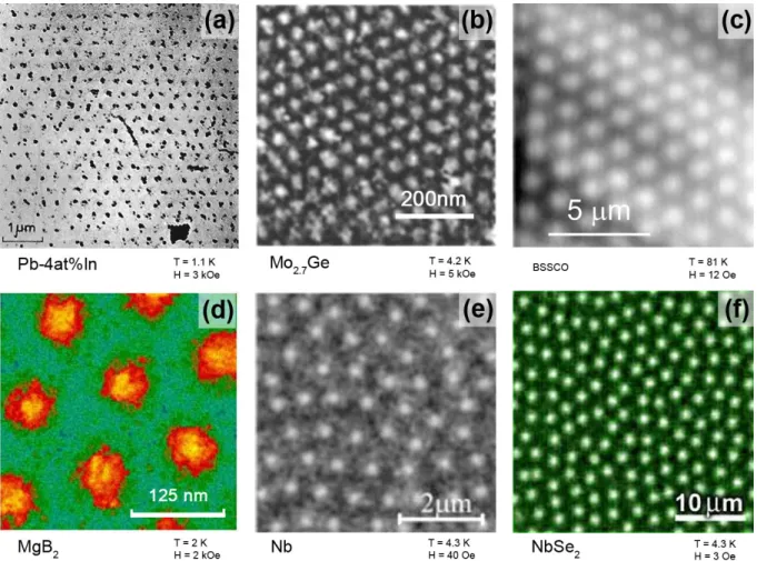
findings have been very important and the vortex lattice is known as the Abrikosov lattice. As examples, Fig. 2.4 shows the Abrikosov lattice observed by different techniques for several materials. Panel (a) shows the first image of the triangular lattice obtained by Bitter decoration in Pb-4at%In rod at T = 1.1 K and H = 3 kOe [38], (b) the lattice in a-Mo2.7Ge thin film taken by Scanning-Tunneling Microscopy (STM) at T = 4.2 K and
H = 5 kOe [39], (c) Scanning Hall Probe Microscopy (SHPM) image taken at T = 81 K andH = 12 Oe in a BSSCO single crystal [40], (d) image obtained from Scanning Tunnel Spectroscopy (STS) for MgB2 single crystal [41] at T = 2 K and H = 2 kOe, (e) image
from Magnetic force microscopy (MFM) in Nb thin film at T = 4.3 K and H = 40 Oe [42], and (f) Magneto-optical imaging (MOI) in NbSe2 single crystal atT = 4.3 K andH
Figure 2.4: Images taken using different techniques to visualize the Abrikosov vortex lattice. (a) Bitter decoration [38], (b) STM [39], (c) SHPM [40], (d) STS [41], (e) MFM [42], and (f) MOI [43], with the conditions and the specimens identified in each panel and also in the text.
As pointed out by Abrikosov, inhomogeneities present in the superconductor influence the overall pattern, as can be seen in Fig. 2.4e and f. Then, the long range order is lost and new vortex phases appear in the mixed state with their own physical properties [36].
2.6
Real superconductors: the pinning centers
The Lorentz force per unit length, Eq.(2.40), acts on an isolated vortex due to the current generated by the other vortices as well as to currents possibly applied to the superconductor. Macroscopically, the lattice starts to move under the action of the Lorentz force density, written as:
FL JB (2.42)
sinceB nϕ0z, where nis the number of vortices and J is the total current density. In a
Fm αmnsevBacts against the Lorentz force, whereη is the friction coefficient,v is
the velocity of the vortex system and αm is the Magnus coefficient. However, an electric
fieldE parallel to J appears due to the velocityvx0, since E Bv. This electric field gives rise to a power dissipation in the system, a consequence of the extra power needed to drive the normal electrons in the moving core, which can be written as [36]
Pd
1
ηJ B
2
(2.43)
and the superconductors would become useless. In order to make them useful, the vortex velocity should be null in spite of a nonzero FL. Thus, the driving Lorentz force should be counteracted by apinning force (Fp). The pinning force defines the maximum critical
current density which a real superconductor can bear without resistance, i.e., without depinning of the vortices. This current density is called critical current density (Jc).
Hence the macroscopic average of the pinning force density can be estimated by:
Fp JcB (2.44)
There is an upper limit for the critical current density which a superconductor can carry. This maximum value is called depairing or pair-breaking critical current density, Jcdepair
orJpb. In the framework of the GL equations,Jcdepair can be obtained by considering the
free energy written only with the kinetic and magnetic field energy contributions for a superconductor with thickness d@ξT. Thus, this ultimate limit is given by:
Jdepair c
ϕ0
3º6πµ0λ2ξ
1 T
Tc
3 2
(2.45)
which is written only in terms of intrinsic and fundamental parameters of the superconductor.
In other words, Jcdepair can be understood as the necessary current to destroy the
Cooper pairs. In real superconductors, however, Jc @Jcdepair since other contributions to
the free energy, such as the loss associated with the vortex motion and the surface barriers for the vortex penetration, should be taken into account.
2.6.1
Intrinsic pinning
dislocations, voids, etc., suppress the superconducting properties (Tc, κ, and
consequently, ψ) at that point or region. They reduce the condensation energy related to the nucleation of the normal core of the vortex and act as attractive potential wells holding the vortices and minimizing the free energy. They cause distortions in the Abrikosov lattice due to the landscape of forces acting on the vortex system and destroying the translational long range order, as illustrated in the Fig. 2.4f. This mechanism of pinning, called core pinning and first described by P. W. Anderson in 1962 [44], is more effective when the dimensions of the inhomogeneities are approximately the coherence lengthξ of the superconducting material.
2.6.2
Artificial pinning
Besides the intrinsic pinning, artificial pinning centers can be introduced in type II superconductors to optimize and trap the vortex lines. It increases the critical current density and consequently, the potential of technological usefulness of the material. One way to insert these defects is by means of irradiating the specimen with high energy heavy ions [45], creating cylinders of non-superconducting material of diameter ξ randomly distributed and with several strengths (or depths). These cylinders are known as columnar defects. These have largely been used in the study of vortex matter in the HTS where
ξ is typically of the order of few nanometers, similar to the size of the defects [46]. Columnar defects can be also obtained by mechanical indentations which are distributed as a periodic array of holes with irregular edges, resulting in pinning centers with different strengths [47].
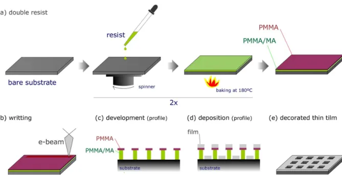
In order to obtain a periodic array of pinning centers almost defect free on the edges, lithographic techniques in thin films have been employed in the last years. The electron beam lithography has allowed one to reach nanometric pinning centers, with controlled size, geometry, and type of defect. There are basically three different types of defects: the antidots¶ (holes through the material) [48, 49, 50], the blind holes (partially drilled holes) [51, 52] and the magnetic dots (magnetic material on top or below the superconductor) [53, 54]. These defects are sketched in Fig 2.5. The superconducting thin films studied here have arrays of antidots.
For these samples, another mechanism to pin vortices becomes important and appear when the distance between the vortex and the antidot is lower than λ. It is called electromagnetic pinning. It takes place due to the perturbation of screening
Figure 2.5: Profile representation of a superconducting thin film (SC) with an array of (a) antidots, (b) blind holes and (c) magnetic dots.
currents of the vortex near the edge superconductor/defect which must flow parallel to the hole edge, because of the boundary condition. Buzdin et al.[55] have calculated this interaction by the method of image, in which a vortex interacts with its image, an antivortex, located in the hole. Therefore, the antidot acts as an attractive potential for the vortex.
Although a multiquanta vortex is energetically unfavorable as shown before, relatively large artificial pinning centers can favor its appearance. Mkrtchyan and Schmidt [56] have found by using London theory that the saturation number of flux quanta nsatT for a
cylindrical hole is given by:
nsatT
R
2ξT (2.46)
where R is the radius of the hole. For an empty hole, the incoming vortex is always attracted to the defect. When 1@n Bnsat, n being the number of flux quanta, the flux
nϕ0 is captured by the hole and creates a potential barrier for other vortices far from
the defect. Increasing the magnetic pressure, for instance, vortices close to the hole can overcome this barrier and enter the hole. WhennAnsat the potential becomes repulsive,
no more flux is accepted into the hole, and the vortices start to occupy interstitial positions in the superconducting region. It is also important to mention thatnsatassumes values of
R~ξT2
in the high-field regime, as recently pointed out by Doria and co-workers [57, 58] using GL theory.
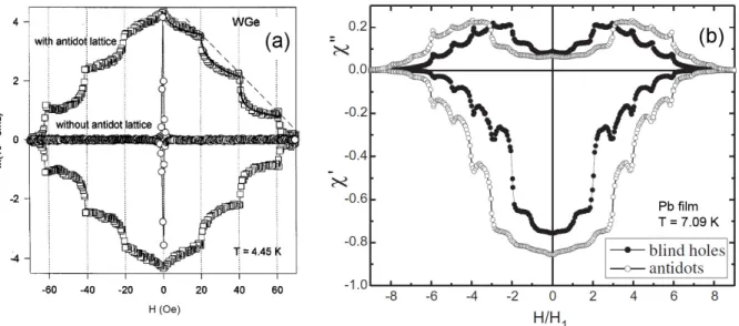
Figure 2.6: Matching fields detected by different techniques. (a) Magnetization versus magnetic field for a decorated W0.77Ge0.33 and a plain film [48] and (b) in phase and out-of phase components of the ac susceptibility for Pb thin filmes with array of holes (open symbols) and blind holes (filled symbol) [51].
fields at which these matching occurs are called matching fields, defined as [59]:
Hn n
ϕ0
µ0A
(2.47)
where A is the unit-cell area of the lattice of defects. At the first matching field H1, for
instance, the equilibrium configuration is one in which each hole is occupied by a single flux quantum on average. Fig. 2.6 shows the matching fields obtained by magnetization and ac susceptibility techniques. Panel (a) shows M(H) curves for a W0.77Ge0.33 thin
film with holes of radius 0.22µm in a square lattice of 1 µm prepared by electron beam lithography whose matching fields are multiples of 20.7 Oe. In the same graph one can see the absence of matching fields on the magnetic response of the plain film. Panel (b) shows both components of ac susceptibility for a Pb thin film with square holes of 0.8
µm in a square lattice of 1.5 µm and blind holes with the same characteristic, both with matching fields in multiples of 9.2 Oe.
2.7
Critical state models: the Bean model
critical current density (Jc).
In the macroscopic point of view, when a magnetic fieldH larger thanHc1 is applied,
currents are induced in the region of the sample where the flux penetrates to counteract the change in the internal magnetic field, in accordance to Maxwell’s equations (Eq. (2.48)). In this region, the macroscopic current is always the maximum current, or the critical current, which the specimen can carry. Therefore, the sample is in the so-called critical state (CS) [60]. From this point of view, it is unnecessary to know any details of the interaction between the vortices and the pinning centers [61]. Nonetheless, the critical state models can be described microscopically. Vortices are nucleated at the edges and penetrate the sample. Since the vortices are captured by the pinning centers, the pinning force acts against the Lorentz force (Eq. 2.42) up to the maximum pinning force (Eq. 2.44). The balance between these two forces (disregarding any other) leads to a local metastable state, where the superconductor employs its maximum current to maintain the flux as close as possible from the edges. Thus, the vortices distribute in such a way that their density decreases from the edge to the center of the specimen. The relation between B
and Jc can be obtained from the Amp`ere law:
© B µ0JcB (2.48)
An important assumption is associated with the relation between B and H. The thermodynamic magnetic field H can be obtained by the Gibbs free energy as
H ∂∂BG B~µ0, considering a type II superconductor with κ Q 1 and Hc2 Q Hc1 [62].
This assumption is related to the region in the Fig 2.2b where B~µ0 merges to H as it
approaches Hc2.
The idea of the critical state and the most simple model was proposed by Charles Bean in 1962 [63], and better discussed in a review published two years later [64]. Bean disregarded the existence of Hc1, i.e., there is no Meissner state in the CS models and
the penetration depth of the flux front should be greater than λ as well. Thus, Bean considered the critical current density as:
JcB, T JcT Bean model (2.49)
i.e., the value of the critical current density at a specific temperature is constant where the flux is penetrated. Above Tc or for HAHc2, the value of Jc is null. Other CS models
model [65], represented respectively by:
JcB, T
J0T
1B~B0T
Kim model (2.50)
JcB, T J0TexpB~B0T Exponential model (2.51)
Although the field dependence of Jc exists, the Bean model is the simplest but a highly
successful tool to determine the critical current density from magnetic and ac susceptibility measurements. In addition to that, the geometric configuration between the field and the specimen affectsJc and the flux distribution inside the sample. Two of the most common
configurations will be discussed in terms of the Bean model: parallel and perpendicular.
2.7.1
Slab/cylinder: parallel configuration
The parallel geometry is related to infinitely long slabs with the dimensions in the y
and z directions much larger than the dimension 2w in the x direction and 2w Q λ or infinitely long cylinders with diameter 2RQ λ. The magnetic field is applied along the z-axis as shown in Fig. 2.7a. In this case, demagnetization effects can be disregarded. Thus, above Hc1 the gradient of the flux density is given by the Amp`ere law as follow:
Jy
∂Hz
∂x ∂Hx
∂z (2.52)
where the second term on the right side is zero for this configuration. Therefore, the critical current is perpendicular to the magnetic field and given by the slopedHz~dx. As
in the Bean modelJy Jc, the gradient of flux density is constant, with the vortex density
B decreasing linearly from the edge to the center of the sample, as illustrated in Fig. 2.7b. By increasing the applied magnetic field from zero upwards, the magnetic induction is given by:
Bzx
¢¨¨¨ ¨¨ ¦¨¨ ¨¨¨¤
0, SxS @a µ0SxS aJc, aB SxS Bw
µ0H, SxS Aw
(2.53)
where a is the distance of the flux front from the center of the specimen. The current density is Jc where the flux is penetrated and null elsewhere:
Jyx ¢¨¨¦¨¨
¤
Jc, a@ SxS Bw
Figure 2.7: Bean model in a slab with width 2win parallel configuration (a). (b) Schematic representation of the microscopic distribution of the vortices in a stripe from the middle of the slab [61]. (c) The magnetic flux profile increasing the field fromH 0, withHp representing the full penetration field and
athe position of the field penetration. (d) The profile of the critical current density for the applied field in the bold line of the case (2). (e) Flux profile when the field is decreased from (5) and (f) profile ofJc
at the case (6).
Fig. 2.7c and d shows the magnetic flux distribution and the critical current density for the applied field labeled as (2). The magnitude of the critical current density can be evaluated when the full penetration field (Hp) is reached, then
Jc
Hp
w (2.55)
Once Hp is reached, the vortex density increases and maintains the same constant
slope. If the applied field is decreased, the vortex density decreases at the edge of the sample, as illustrated in Fig. 2.7e, with the slope dHz~dx. The critical current density
changes the sign, although its magnitude remains the same in accordance with the assumption of the model (Fig. 2.7f).
2.7.2
Thin film: perpendicular configuration
The reduction of one (or more) dimensions gives rise to different flux and critical current distributions in superconducting systems. For a thin film geometry, considering a small ratio between the thickness and the London penetration depth (d~λ), i. e.,
d P λ, the structure of the vortices acquires different properties from those of the superconducting bulk, if it is placed in a perpendicular or transverse configuration (the applied field is normal to the specimen surface as in Fig. 2.8a). J. Pearl [66] assumed
Figure 2.8: Long stripe and thin disk representing a thin film in a perpendicular geometry (a), withw
being half of stripe width, R is the disk radius and d is the thickness. Magnetic flux profile (b) and current density (c) in the cases (1) through (4).
can be written as:
j 1
µ0Λ
Aδz (2.56) with
ΛT 2 λT
2
d (2.57)
where λT is the bulk penetration depth. As a consequence of the two-dimensional features, a new length scale controls the spatial variation of J (and A), named effective penetration depth, Λ. It means that the thin-film vortices have an electromagnetic interaction of longer range, compared to the three-dimensional case (Eq. (2.15)), since Λ Q λ. The radius of the vortex core is the same ξT as in a bulk sample, but the gradual decrease of the current around the vortex is more spread out and consequently, the magnetic field also decays in a longer length [27, 33]. Thus, non-local effects should be taken into account. This becomes clear comparing both geometries: for r Q Λ, the current decreases as 1~r2
, whereas for a bulk, it decreases as er~λ for r Q λ,
remembering that the relevant scale for thin films is ΛQλ. The local magnetic field and the intervortex force cut-off as 1~r3
(for r Q Λ) and 1~r2
for a thin film, respectively, whereas both cut-off exponentially for a bulk.
by Λ. For instance, tin and lead in bulk shape are type I superconductors, nonetheless in thin film with thickness less than the critical value of around 180 nm and 250 nm, respectively, they behave as type II superconductors [67].
The description of the Bean model for the flux and current profiles for a slab geometry (Fig. 2.7) is no longer valid for a thin film in perpendicular configuration. The superconducting thin films show large demagnetization effects influencing the magnetic response due to magnetic poles appearing on the surface of the thin film. In this case, the internal field is equal to the applied field H corrected by the demagnetization field
Hd, that is [68]:
HN HHd HNM (2.58) where N is the demagnetization tensor and T rN 1. Thus, the constitutive relation of the magnetism becomes:
B µ0H 1
NM (2.59) The demagnetization factor depends on the shape of the specimen and of the orientation relative to the magnetic field. For samples in the format of ellipsoids of revolution, the demagnetization tensor can be treated as a scalar demagnetization factor N. For an infinite cylinder with the magnetic field parallel to the main axis, N is null (no demagnetization factor), whereas in a perpendicular geometry, N is 2~3. For a sphere, the value of N 1~3. For a superconducting thin film in perpendicular configuration, an oblate ellipsoid is used to model N through the ratio between major axis w and the minor axisd, given by γ d~w. For small γ,N is:
N 11
2πγ2γ
2
(2.60)
which results inN 1 for the thin films studied here. Consequently, it enables vortices to come into the thin film at applied fields smaller than the bulk lower critical field (Hbulk
c1 ),
given by:
Hcf ilm1
¾
d wH
bulk
c1 (2.61)
decreasing the value of Hc1 for the thin film geometry.
Another consequence of strong demagnetization effects is that magnetic flux lines wrap around the thin film and originate in-plane components of Hx with the opposite sign on
the top and bottom surfaces, i.e., Hxx, z d~2 Hxx, z d~2. It also leads to a
larger gradient of ∂Hx
∂z than the term ∂Hz
Consequently, the effective magnetic field at the edges is higher than the applied magnetic field, and the screening currents flow everywhere in the sample. There are two geometries where superconducting thin films are depicted: an infinitely long stripe with the width of 2w and a thin disk with the radiusR, the schematic representation of which are shown in Fig. 2.8a . When the applied field is increased from zero, the magnetic field around the long stripe is [62, 69]:
Bzx
¢¨¨¨ ¨¨¨¨ ¦¨¨ ¨¨¨¨¨ ¤
0, SxS @a µ0HgarctanhSwxSx
2
a2
w2a2
1~2
, a@ SxS @w µ0HgarctanhS
xS w
w2
a2
x2a2
1~2
, SxS Aw
(2.62)
and as the current density is given by:
Jyx ¢¨¨¨¦¨¨
¨¤
JcSxxS, a@ SxS @w
2Jc
π arctan x w
w2
a2
a2x2
1~2
, SxS @a (2.63)
wherea is the position of the flux front written as:
a w
coshH Hg
(2.64)
and for a long stripe, the characteristic field Hg is
Hg Jπcd long stripe (2.65)
For a thin disk [70], the magnetic flux and the current profiles are approximately the same as shown in Eq. (2.63) and (2.62), except by replacing the following parameters [71]:
xÐ r
wÐ R thin disk
Hg J2cd
(2.66)
hence both geometries are similar unidimensional problems. Fig. 2.8b shows the magnetic flux profile when the applied field is raised for different values and the panel (c) shows the current density profile. The current is constant and equals to Jc where the field is
penetrated, whereas Meissner currents flow in the flux-free region [72].
The kind of configuration based on the alignment between the specimen and the magnetic field is determined by thickness and the penetration depth [73]. For the situation where d A w Q λ, the Bean model in the parallel orientation can be employed. For
therefore, the perpendicular configuration should be considered.
![Figure 2.7: Bean model in a slab with width 2w in parallel configuration (a). (b) Schematic representation of the microscopic distribution of the vortices in a stripe from the middle of the slab [61]](https://thumb-eu.123doks.com/thumbv2/123dok_br/15760112.639494/44.892.96.758.108.367/figure-parallel-configuration-schematic-representation-microscopic-distribution-vortices.webp)

![Figure 3.3: Dendritic morphology of the avalanches in thin films visualized by MOI: (a) YBCO after a laser pulse [89, 90]; (b) Nb decreasing the field after a field cooled procedure at H = 135 Oe [91]; (c) MgB 2 increasing the magnetic field [92, 93]; Nb 3](https://thumb-eu.123doks.com/thumbv2/123dok_br/15760112.639494/54.892.81.767.132.623/dendritic-morphology-avalanches-visualized-decreasing-procedure-increasing-magnetic.webp)