Off-Diagonal Mass Generation for Yang-Mills Theories in the Maximal Abelian Gauge
D. Dudala,∗J.A. Graceyb, V.E.R. Lemesc, M.S. Sarandyd, R.F. Sobreiroc, S.P. Sorellac,†and H. Verscheldea a Ghent University, Department of Mathematical Physics and Astronomy,
Krijgslaan 281-S9, B-9000 Gent, Belgium
b Theoretical Physics Division,
Department of Mathematical Sciences, University of Liverpool, P.O. Box 147, Liverpool, L69 3BX, United Kingdom
c UERJ - Universidade do Estado do Rio de Janeiro Rua S˜ao Francisco Xavier 524, 20550-013,
Maracan˜a, Rio de Janeiro, Brazil
d Chemical Physics Theory Group, Department of Chemistry,
University of Toronto, 80 St. George Street, Toronto, Ontario, M5S 3H6, Canada
Received on 12 December, 2006
We investigate a dynamical mass generation mechanism for the off-diagonal gluons and ghosts inSU(N) Yang-Mills theories, quantized in the maximal Abelian gauge. Such a mass can be seen as evidence for the Abelian dominance in that gauge. It originates from the condensation of a mixed gluon-ghost operator of mass dimension two, which lowers the vacuum energy. We construct an effective potential for this operator by a combined use of the local composite operators technique with algebraic renormalization and we discuss the gauge parameter independence of the results. We also show that it is possible to connect the vacuum energy, due to the mass dimension two condensate discussed here, with the non-trivial vacuum energy originating from the condensateA2µ®, which has attracted much attention in the Landau gauge.
Keywords: Gauge theory; BRST quantization; Renormalization group; Nonperturbative effects
I. INTRODUCTION.
An unresolved problem of SU(N) Yang-Mills theory is color confinement. A physical picture that might explain con-finement is based on the mechanism of the dual supercon-ductivity [1, 2], according to which the low energy regime of QCDshould be described by an effective Abelian theory in the presence of magnetic monopoles. These monopoles should condense, giving rise to the formation of flux tubes which confine the chromoelectric charges.
Let us provide a very short overview of the concept of Abelian gauges, which are useful in the search for magnetic monopoles, a crucial ingredient in the dual superconductivity picture.
Abelian gauges
We recall thatSU(N)has aU(1)N−1subgroup, consisting
of the diagonal generators. In [2], ’t Hooft proposed the idea of the Abelian gauges. Consider a quantityX(x), transforming
∗Talk given by D. Dudal at “XXV Encontro Nacional de F´ısica de Part´ıculas
e Campos”, Caxambu, Minas Gerais, Brazil, 24-28 Aug 2004; Research As-sistant of the Fund For Scientific Research-Flanders (Belgium)
†Work supported by FAPERJ, Fundac¸˜ao de Amparo `a Pesquisa do
Es-tado do Rio de Janeiro, under the programCientista do Nosso Estado, E-26/151.947/2004.
in the adjoint representation ofSU(N).
X(x)→U(x)X(x)U+(x)withU(x)∈SU(N). (1) The transformationU(x)which diagonalizesX(x)is the one that defines the gauge. IfX(x)is already diagonal, then clearly X(x)remains diagonal under the action of theU(1)N−1
sub-group. Hence, the gauge is only partially fixed because there is a residual Abelian gauge freedom.
In certain space time points xi, the eigenvalues of X(x)
can coincide, so thatU(xi)becomes singular. These possible
singularities give rise to the concept of (Abelian) mag-netic monopoles. They have a topological meaning since π2¡SU(N)/U(1)N−1¢6=0 and we refer to [3, 4] for all the
necessary details.
The dual superconductor as a mechanism behind con-finement
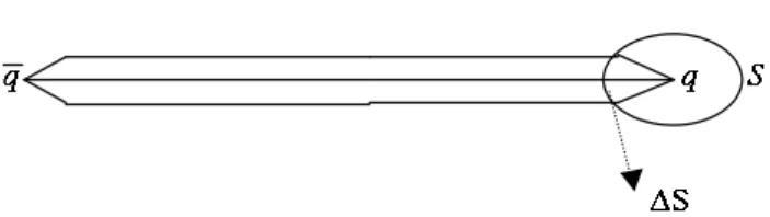
Let us give a simplified picture of the dual superconductor to explain the idea. If theQCDvacuum contains monopoles and if these monopoles condense, there will be a dual Meiss-ner effect which squeezes the chromoelectric field into a thin flux tube. This results in a linearly rising potential,V(r) =σr, between static charges, as can be guessed from Gauss’ law, R
FIG. 1: A chromoelectric flux tube between a static quark-antiquark pair.
An example of an Abelian gauge: the maximal Abelian gauge (MAG)
Let Aµ be the Lie algebra valued connection for the
gauge group SU(N), whose generators TA, satisfying
£
TA,TB¤ = fABCTC, are chosen to be antihermitean and to obey the orthonormality condition Tr¡TATB¢=−TFδAB,
withA,B,C=1, . . . ,¡N2−1¢. In the case ofSU(N), one has TF =12. We decompose the gauge field into its off-diagonal
and diagonal parts, namely
Aµ=AAµTA=AµaTa+AiµTi, (2)
where the indicesi,j,. . .label theN−1 generators of the Car-tan subalgebra. The remainingN(N−1)off-diagonal genera-tors will be labeled by the indicesa,b,. . .. The field strength decomposes as
Fµν=FµAνTA=FµaνTa+FµiνTi, (3) with the off-diagonal and diagonal parts given respectively by Fµaν = Dabµ Abν−DνabAbµ +g fabcAbµAcν, (4) Fµiν = ∂µAiν−∂νAiµ+g fabiAaµAbν,
where the covariant derivativeDabµ is defined with respect to the diagonal componentsAiµ
Dabµ ≡∂µδab−g fabiAiµ . (5)
For the Yang-Mills action one obtains
SYM=−
1 4 Z
d4x¡FµaνFµνa+FµiνFµνi¢. (6)
The maximal Abelian gauge (MAG), introduced in [2–4], cor-responds to minimizing the functional
R
[A] = Zd4x£AaµAµa¤ (7)
One checks that
R
[A]does exhibit a residualU(1)N−1invari-ance.
The MAG can be recast into a differential form
DabµAµb=0 (8)
Although we have introduced the MAG here in a functional way, it is worth mentioning that the MAG does correspond to the diagonalization of a certain adjoint operator, see e.g. [5].
The renormalizability in the continuum of the MAG was proven in [6, 7], at the cost of introducing a quartic ghost in-teraction. The corresponding gauge fixing term turns out to be [6, 7]
SMAG=s
Z d4x
³
ca
³
DabµAbµ+α 2b
a´ −α
2g f
abicacbci −α
4g f
abccacbcc´,
(9) whereαis the MAG gauge parameter andsdenotes the nilpotent BRST operator, acting as
sAaµ = −³Dabµcb+g fabcAbµcc+g fabiAbµci
´
, sAiµ=−³∂µci+g fiabAaµcb ´
,
sca = g fabicbci+g 2f
abccbcc, sci=g
2 f
iabcacb,
sca = ba, sci=bi,
sba = 0, sbi=0. (10)
Hereca,ciare the off-diagonal and the diagonal components of the Faddeev-Popov ghost field, whileca,baare the off-diagonal
antighost and Lagrange multiplier. We also observe that the BRST transformations(10)have been obtained by their standard form upon projection on the off-diagonal and diagonal components of the fields. We remark that the MAG (9) can be written in the form
SMAG=ss
Z d4x
µ
1 2A
a µAµa−
α 2c
aca ¶
withsbeing the nilpotent anti-BRST transformation, acting as sAaµ = −³Dabµ cb+g fabcAbµcc+g fabiAbµci
´
, sAiµ=−³∂µci+g fiabAaµcb ´
,
sca = g fabicbci+g 2f
abccbcc, sci=g
2 f
iabcacb,
sca = −ba+g fabccbcc+g fabicbci+g fabicbci, sci=−bi+g fibccbcc,
sba = −g fabcbbcc−g fabibbci+g fabicbbi sbi=−g fibcbbcc. (12) It can be checked thatsandsanticommute.
Expression(9)is easily worked out and yields SMAG =
Z d4x
³
ba
³
Dabµ Aµb+α 2b
a´+caDab
µDµbccc+gcafabi ³
DbcµAµc
´
ci+gcaDabµ
³
fbcdAµccd
´
− αg fabibacbci−g2fabifcdicacdAbµAµc−α 2g f
abcbacbcc −α
4g
2fabifcdicacbcccd
− α 4g
2fabcfadicbcccdci−α
8g
2fabcfadecbcccdce´. (13)
We note thatα=0 does in fact correspond to the “real” MAG condition, given by eq.(8). However, one cannot set α=0 from the beginning since this would lead to a nonrenor-malizable gauge. Some of the terms proportional toαwould reappear due to radiative corrections, even ifα=0. See, for example, [30]. For our purposes, this means that we have to keepαgeneral throughout and leave to the end the analysis of
the limitα→0, to recover condition (8).
In order to have a complete quantization of the theory, one has to fix the residual Abelian gauge freedom by means of a suitable further gauge condition on the diagonal components Aiµof the gauge field. A common choice for the Abelian gauge fixing, also adopted in the lattice papers [5, 8], is the Landau gauge, given by
Sdiag=s
Z
d4x ci∂µAµi =
Z
d4x ³bi∂µAµi+ci∂µ ³
∂µci+g fiabAaµcb ´´
, (14)
whereci,bi are the diagonal antighost and Lagrange multi-plier.
Abelian dominance
According to the concept of Abelian dominance, the low energy regime of QCD can be expressed solely in terms of Abelian degrees of freedom [9]. Lattice confirmations of the Abelian dominance can be found in [10, 11]. To our knowl-edge, there is no analytic proof of the Abelian dominance. Nevertheless, an argument that can be interpreted as evidence of it, is the fact that the off-diagonal gluons would attain a dy-namical mass. At energies below the scale set by this mass, the off-diagonal gluons should decouple, and in this way one should end up with an Abelian theory at low energies.
A lattice study of such an off-diagonal gluon mass reported a value of approximately 1.2GeV [5]. More recently, the off-diagonal gluon propagator was investigated numerically in [8], reporting a similar result.
There have been several efforts to give an analytic descrip-tion of the mechanism responsible for the dynamical gen-eration of the off-diagonal gluon mass. In [12, 13], a cer-tain ghost condensate was used to construct an effective,
off-diagonal mass. However, in [14] it was shown that the ob-tained mass was a tachyonic one, a fact confirmed later in [15]. Another condensation, namely that of the mixed gluon-ghost operator(1
2A a
µAµa+αcaca)[39], that could be responsible for
the off-diagonal mass, was proposed in [16]. That this oper-ator should condense can be expected on the basis of a close analogy existing between the MAG and the renormalizable nonlinear Curci-Ferrari gauge [17, 18]. In fact, it turns out that the mixed gluon-ghost operator can be introduced also in the Curci-Ferrari gauge. A detailed analysis of its conden-sation and of the ensuing dynamical mass generation can be found in [19, 20].
Here, we shall report on the results of [21]. It was investi-gated explicitly if the mass dimension two operator(1
2A a µAµa+ αcaca)condenses, so that a dynamical off-diagonal mass is
generated in the MAG. The pathway we intend to follow is based on previous research in this direction in other gauges. In [22], the local composite operator (LCO) technique was used to construct a renormalizable effective potential for the operatorAAµAµA in the Landau gauge. As a consequence of
AAµAµA®6=0, a dynamical mass parameter is generated [22]. The condensateAA
µAµA ®
theoret-ical [23, 24] as well as from the lattice side [25]. It was shown by means of the algebraic renormalization technique [26] that the LCO formalism for the condensateAA
µAµA ®
is renormal-izable to all orders of perturbation theory [27]. The same for-malism was successfully employed to study the condensation of(1
2A A
µAµA+αcAcA)in the Curci-Ferrari gauge [19, 20]. We
would like to note that the Landau gauge corresponds toα=0. Later on, the condensation ofAA
µAµAwas confirmed in the
lin-ear covariant gauges [28, 29], which also possess the Landau gauge as a special case. It was proven formally that the va-cuum energy does not depend on the gauge parameter in these gauges. As such, the linear, Curci-Ferrari and Landau gauges are all connected to each other. We managed to connect also the MAG with the Landau gauge, and as such with the linear and Curci-Ferrari gauges [21].
II. RENORMALIZABILITY OFSU(N)YANG-MILLS THEORIES IN THE MAG IN THE PRESENCE OF THE
LOCAL COMPOSITE OPERATOR(1
2AaµAµa+αcaca)
To prove the renormalizability to all orders of perturbation theory, we shall rely on the algebraic renormalization formal-ism [26]. In order to write down a suitable set of Ward identi-ties, we first introduce external fieldsΩµi,Ωµa,Li,Lacoupled
to the BRST nonlinear variations of the fields, namely
Sext=
Z
d4x³−Ωµa³Dab
µ cb+g fabcAbµcc+g fabiAbµci ´
−Ωµi³∂
µci+g fiabAaµcb ´
+La³g fabicbci+g 2f
abccbcc´+Lig
2 f
iabcacb´, (15)
with
sΩµa = sΩµi=0, (16)
sLa = sLi=0.
Moreover, in order to discuss the renormalizability of the gluon-ghost operator
O
MAG=1 2A
a
µAµa+αcaca, (17)
we introduce it in the starting action by means of a BRST doublet of external sources(J,λ)
sλ=J, sJ=0, (18)
so that
SLCO = s
Z d4x
µ
λ
µ
1 2A
a
µAµa+αcaca ¶
+ζλJ 2
¶
(19)
= Z
d4x
µ
J
µ
1 2A
a
µAµa+αcaca ¶
+ζJ 2
2 −αλb
aca
+ λAµa³Dabµ cb+g fabiAbµci
´
+αλca³g fabicbci+g 2f
abccbcc´´,
whereζis the LCO parameter accounting for the divergences present in the vacuum correlatorh
O
MAG(x)O
MAG(y)i, whichare proportional toJ2. Therefore, the complete action Σ=SYM+SMAG+Sdiag+Sext+SLCO, (20)
is BRST invariant
sΣ=0. (21)
It is worth mentioning that the mixed gluon-ghost mass opera-tor, defined in eq.(17), is built using off-diagonal components only. As noticed in [16, 31], the operator (17) is also BRST invariant on-shell. We have written down in [21] all the Ward identities, which are sufficient to prove that the most gen-eral local counterterm, compatible with the symmetries of the model, can always be reabsorbed by means of multiplicative renormalization. As an interesting by-product, we have been
able to establish a relation between the anomalous dimension of the gluon-ghost operator
O
MAG and other, moreelemen-tary, renormalization group functions. Explicitly, it holds to all orders of perturbation theory that
γOMAG(g
2) =−2 µ
β(g2)
2g2 −γci(g2) ¶
, (22)
whereβ(g2) =µ∂∂gµ2 andγci(g2)denotes the anomalous
dimen-sion of the diagonal ghost field.
A. The effective potential via the LCO method.
To obtain the effective potential for the condensateh
O
MAGi,we set the sourcesΩi
µ,Ωaµ,La,Liandλto zero and consider
the renormalized generating functional
exp(−i
W
(J)) = Z[Dϕ]expiS(J),
S(J) = SYM+SMAG+Sdiag+Scount+
Z d4x
µ
ZJJ µ
1 2ZeAA
a
µAµa+ZαZecαcaca ¶
+ (ζ+δζ)J
2
2
¶
, (23) whereϕdenotes the relevant fields andScountis the usual counterterm contribution, i.e. the part without the composite operator
O
MAG. The quantityδζis the counterterm accounting for the divergences proportional toJ2. Using dimensional regularizationthroughout with the convention thatd=4−ε, one has the following identification
ζ0J02=µ−ε(ζ+δζ)J2. (24)
where the subscript “0” denotes bare quantities. The functional
W
(J)obeys the renormalization group equation (RGE)µ
µ ∂ ∂µ+β(g
2) ∂
∂g2+αγα(g 2) ∂
∂α−γOMAG(g
2)Z d4xJ δ δJ+η(g
2,ζ)∂ ∂ζ
¶
W
(J) =0, (25)where
γα(g2) = µ ∂ ∂µlnα, η(g2,ζ) = µ ∂
∂µζ. (26)
Acting withµ∂∂µon eq.(24) and keeping in mind that bare quantities do not depend on the renormalization scaleµ, one finds
η(g2,ζ) =2γOMAG(g2)ζ+δ(g2,α), (27)
with
δ(g2,α) =
µ
ε+2γOMAG(g
2)
−β(g2) ∂
∂g2−αγα(g 2) ∂
∂α
¶
δζ. (28)
Up to now, the LCO parameterζis still an arbitrary coupling. As explained in [32, 33], simply settingζ=0 would give rise to an inhomogeneous RGE for
W
(J)µ
µ ∂ ∂µ+β(g
2) ∂
∂g2+αγα(g 2) ∂
∂α−γOMAG(g
2)Z d4xJ δ δJ
¶
W
(J) =δ(g2,α) Zd4xJ 2
2 , (29)
and a non-linear RGE for the associated effective action Γ for the composite operator
O
MAG. Furthermore,multiplica-tive renormalizability is lost and by varying the value ofδζ, minima of the effective action can change into maxima or can get lost. However,ζ can be made such a function ofg2and
αso that, ifg2runs according to β(g2)andαaccording to γα(g2),ζ(g2,α)will run according to its RGE (27). This is accomplished by settingζequal to the solution of the differ-ential equation
µ
β(g2) ∂
∂g2+αγα(g 2,α) ∂
∂α
¶
ζ(g2,α) =2γOMAG(g
2)ζ(g2,α) +δ(g2,α).
(30) Doing so,
W
(J)obeys the homogeneous renormalization group equationµ
µ ∂ ∂µ+β(g
2) ∂
∂g2+αγα(g 2) ∂
∂α−γOMAG(g
2)Z d4xJ δ δJ
¶
To lighten the notation, we will drop the renormalization factorsZJ,ZeA, etc. from now on. One will notice that there are terms
quadratic in the sourceJpresent in
W
(J), obscuring the usual energy interpretation. This can be cured by removing the terms proportional toJ2in the action to get a generating functional that is linear in the source, a goal easily achieved by inserting thefollowing unity,
1= 1
N Z
[Dσ]exp
"
i Z
d4x
Ã
−1 2ζ
µ
σ
g−
O
MAG−ζJ¶2!#
, (32)
withNthe appropriate normalization factor, in eq.(23) to arrive at the Lagrangian
L
(Aµ,σ) =−1 4Fa µνFµνa−
1 4F
i
µνFµνi+
L
MAG+L
diag− σ22g2ζ+
1
g2ζgσ
O
MAG−1
2ζ(
O
MAG) 2, (33)
while
exp(−i
W
(J)) = Z[Dϕ]expiSσ(J), (34) Sσ(J) =
Z d4x
µ
L
(Aµ,σ) +Jσ g¶
. (35)
From eqs.(23) and (34), one has the following simple relation δ
W
(J)δJ
¯ ¯ ¯
¯J=0=−h
O
MAGi=− ¿σ g
À
, (36)
meaning that the condensateh
O
MAGiis directly related to theexpectation value of the field σ, evaluated with the action Sσ=Rd4x
L
(Aµ,σ). As it is obvious from eq.(33),hσi 6=0 is sufficient to have a tree level dynamical mass for the off-diagonal fields. At lowest order (i.e. tree level), one findsmoffgluon−diag. =
r
gσ ζ0
, moffghost−diag.=
r
αgσ ζ0
. (37)
Meanwhile, the diagonal degrees of freedom remain massless.
III. GAUGE PARAMETER INDEPENDENCE OF THE VACUUM ENERGY.
We begin this section with a few remarks on the determi-nation ofζ(g2,α). From explicit calculations in perturbation theory, it will become clear [40] that the RGE functions show-ing up in the differential equation (30) look like
β(g2) = −εg2−2¡β0g2+β1g2+··· ¢
,
γOMAG(g
2) = γ
0(α)g2+γ1(α)g4+···, γα(g2) = a0(α)g2+a1(α)g4+···,
δ(g2,α) = δ0(α) +δ1(α)g2+···. (38)
As such, eq.(30) can be solved by expanding ζ(g2,α)in a Laurent series ing2,
ζ(g2,α) =ζ0(α)
g2 +ζ1(α) +ζ2(α)g
2+···. (39)
More precisely, for the first coefficientsζ0,ζ1of the
expres-sion (39), one obtains 2β0ζ0+αa0
∂ζ0
∂α = 2γ0ζ0+δ0, 2β1ζ0+αa0
∂ζ1 ∂α +αa1
∂ζ0
∂α = 2γ0ζ1+2γ1ζ0+δ1.(40) Notice that, in order to construct then-loop effective potential, knowledge of the(n+1)-loop RGE functions is needed.
The effective potential calculated with the Lagrangian (33) will explicitly depend on the gauge parameterα. The question arises concerning the vacuum energyEvac, (i.e. the effective
potential evaluated at its minimum); will it be independent of the choice ofα? Also, as it can be seen from the equations (40), eachζi(α)is determined through a first order
differen-tial equation inα. Firstly, one has to solve forζ0(α). This
will introduce one arbitrary integration constantC0. Using
the obtained value forζ0(α), one can consequently solve the
first order differential equation forζ1(α). This will introduce
a second integration constantC1, etc. In principle, it is
possi-ble that these arbitrary constants influence the vacuum energy, which would represent an unpleasant feature. Notice that the differential equations inαfor theζiare due to the running of αin eq.(30), encoded in the renormalization group function γα(g2). Assume that we would have already shown thatEvac
does not depend on the choice ofα. If we then setα=α∗, withα∗a fixed point of the RGE forα at the considered or-der of perturbation theory, then equation (30) determiningζ simplifies to
β(g2) ∂
∂g2ζ(g 2,α∗) =
2γOMAG(g2)ζ(g2,α∗)+δ(g2,α∗), (41)
since
γα(g2)α ¯ ¯
α=α∗=0. (42)
This will lead to simple algebraic equations for theζi(α∗).
Hence, no integration constants will enter the final result for the vacuum energy forα=α∗, and sinceEvacdoes not depend
onα,Evacwill never depend on the integration constants, even
Summarizing, two questions remain. Firstly, we should prove that the value ofαwill not influence the obtained value forEvac. Secondly, we should show that there exists a fixed
pointα∗. We postpone the discussion concerning the second
question to the next section, giving a positive answer to the first one. In order to do so, let us reconsider the generating functional (34). We have the following identification, ignor-ing the overall normalization factors
exp(−i
W
(J)) = Z[Dϕ]expiSσ(J) = 1 N Z
[DϕDσ]expi
"
S(J) + Z
d4x
Ã
−1 2ζ
µ
σ
g−
O
MAG−ζJ¶2!#
, (43)
whereS(J)andSσ(J)are given respectively by eq.(23), and eq.(35). Obviously, d
dα 1 N Z
[Dσ]exp
"
i Z
d4x
Ã
−1 2ζ
µ
σ
g−
O
MAG−ζJ¶2!#
= d
dα1=0, (44)
so that d
W
(J)dα =−
¿
s Z
d4xs
µ
1 2c
aca¶À¯¯¯ ¯
J=0
+terms∝J, (45)
which follows directly from dS(J)
dα =ss Z
d4x
µ
1 2c
aca ¶
+terms∝J. (46)
The terms proportional to the sourceJ are originating from the term 12ζJ2present in eq.(23).
We see that the first term in the right hand side of (46) is an exact BRST variation. As such, its vacuum expectation value vanishes. This is the usual argument to prove the gauge parameter independence in the BRST framework [26]. Note that no local operator ˆ
O
, withsO
ˆ =O
MAG, exists.Further-more, extending the action of the BRST transformation on the σ-field by
sσ=gs
O
MAG=−AµaDabµ cb+αbaca−αg fabicacbci−α
2g f
abccacbcc (47)
one can easily check that s
Z
d4x
L
(Aµ,σ) =0, (48) so that we have a BRST invariantσ-action. Thus, when we consider the vacuum, corresponding toJ=0, only the BRST exact term in eq.(45) survives. The effective actionΓis re-lated toW
(J) through a Legendre transformationΓ³σg´=−
W
(J)−Rd4yJ(y)σ(y)g , while the effective potentialV(σ)is defined as−V(σ) Z
d4x=Γ
µ
σ g
¶
. (49)
Ifσminis the solution of dV(dσσ) =0, then it follows from δ
δ³σg´
Γ=−J, (50)
that
σ=σmin⇒J=0, (51)
and hence, d dαV(σ)
¯ ¯ ¯ ¯σ
=σmin
Z
d4x= d
dα
W
(J)¯ ¯ ¯ ¯
J=0
, (52)
or, due to eq.(45), d dαV(σ)
¯ ¯ ¯ ¯
σ=σmin
=0. (53)
We conclude that the vacuum energyEvacshould be
indepen-dent from the gauge parameterα.
A completely analogous derivation was performed in the case of the linear gauge [29]. Nevertheless, in spite of the previous argument, explicit results in that case showed that Evacdid depend onα. In [29] it was argued that this apparent
disagreement was due to a mixing of different orders of per-turbation theory. We explain this with a simple example. A key argument in the previous analysis is that the sourceJ=0 vanishes at the end of the calculations. In practice,J=0 is achieved by solving the gap equation dVdσ =0. Perturbation theory corresponds to a power series expansion in the cou-pling constant. The derivative of the effective potential with respect toσwill hence look like
¡
v0+v1g2+O(g4) ¢
σ, (54)
where we assume that we work up to orderg2. The correspon-ding gap equation reads
Due to eqs.(49) and (50), one also has J=g¡v0+v1g2+O(g4)
¢
σ. (56)
Imposing the gap equation (55) leads to
J=g¡0+O(g4)¢σ. (57) However, as it can be immediately checked from expression (43), there are several terms proportional toJin the right-hand side of eq.(45). For instance, one of them is given by ∂α∂ζJ2. Since
∂ζ ∂α=
∂ζ0 ∂α
1 g2+
∂ζ1 ∂α +O(g
2), (58)
we find ∂ζ ∂αJ
2= µ∂ζ
0 ∂αv
2 0+
µ∂ζ 0 ∂α2v0v1+
∂ζ1 ∂αv
2 0 ¶
g2+O(g4)
¶
σ2.
(59) Squaring the gap equation (55),
v20+2v1v0g2+O(g4) =0, (60)
leads to
∂ζ ∂αJ
2= µ
∂ζ1 ∂αv
2
0g2+O(g4) ¶
σ2. (61)
We see that, if one consistently works to the first order, terms such as ∂α∂ζJ2do not equal zero, althoughJ=0 to that order. Terms like those on the right-hand side of eq.(61) are can-celed by terms which are formally of higher order, requiring thus a mixing of different orders of perturbation theory. Of course, this problem would not have occurred if we were be able to compute the effective potential up to infinite order. We proposed a modification of the LCO formalism suitable cir-cumventing this problem and obtaining a well defined gauge independent vacuum energyEvac, without the need of working
at infinite order [29]. Instead of the action (23), let us consider the following action
e
S(Je) = SYM+SMAG+Sdiag+
Z d4x
· e
J
F
(g2,α)O
MAG+ ζ 2F
2(g2,α)Je2 ¸
, (62)
where, for the moment,
F
(g2,α)is an arbitrary function ofαof the formF
(g2,α) =1+f0(α)g2+f1(α)g4+O(g6), (63)andJeis now the source. The generating functional becomes exp(−i
W
f(Je)) =Z
[Dφ]expiSe(Je). (64)
Taking the functional derivative of
W
f(Je)with respect toJe, we obtain δW
f(Je)δJe
¯ ¯ ¯ ¯ ¯e
J=0
=−
F
(g2,α)hO
MAGi. (65)Once more, we insert unity via
1= 1
N Z
[Deσ]exp
"
i Z
d4x
Ã
−1 2ζ
µ e
σ
g
F
(g2,α)−O
MAG−ζJeF
(g 2,α)¶2!#
, (66)
to arrive at the following Lagrangian
e
L
(Aµ,eσ) =−1 4Fa µνFµνa−
1 4F
i
µνFµνi+
L
MAG+L
diag− e σ22g2
F
2(g2,α)ζ+1
g2
F
(g2,α)ζgeσO
MAG−1
2ζ(
O
MAG) 2.(67)
From the generating functional exp(−i
W
f(Je)) =Z
[Dφ]expiSσe(Je), (68) Sσe(Je) =
Z d4x
µ
L
(Aµ,eσ) +Jeσe g¶
. (69)
it follows that δ
W
f(Je)δJe
¯ ¯ ¯ ¯ ¯e
J=0
=−
¿ e
σ g
À
The renormalizability of the action (35) implies that the ac-tion (69) will be renormalizable too. Notice indeed that both actions are connected through the transformation
e
J = J
F
(g2,α). (71)The tree level off-diagonal masses are now provided by
moffgluon−diag. =
s
geσ ζ0
, moffghost−diag.=
s
αgσe ζ0
, (72)
while the vacuum configuration is determined by solving the gap equation
dVe(eσ)
deσ =0, (73)
withVe(eσ)the effective potential. MinimizingVe(σe)will lead to a vacuum energyEvac(α)which will depend onαand the
hitherto undetermined functions fi(α)[41]. We will
deter-mine those functions fi(α) by requiring that Evac(α) is α
-independent. More precisely, one has
dEvac
dα =0⇒first order differential equations inαfor fi(α). (74) Of course, in order to be able to determine the fi(α), we
need an initial value for the vacuum energyEvac. This
cor-responds to initial conditions for the fi(α). In the case of
the linear gauges, to fix the initial condition we employed the Landau gauge [29], a choice which would also be possible in case of the Curci-Ferrari gauges, since the Landau gauge be-longs to these classes of gauges. This choice of the Landau gauge can be motivated by observing that the integrated oper-atorRd4xAAµAµAhas a gauge invariant meaning in the Landau gauge, due to the transversality condition∂µAµA=0, namely
(V T)−1 min
UεSU(N)
Z
d4xh¡AAµ¢U¡AµA¢U
i
= Z
d4x(AAµAµA) in the Landau gauge, (75) with the operator on the left hand side of eq.(75) being gauge invariant. Moreover, the Landau gauge is also an all-order fixed point of the RGE for the gauge parameter in case of the linear and Curci-Ferrari gauges. At first glance, it could seem that it is not possible anymore to make use of the Landau gauge as initial condition in the case of the MAG, since the Landau gauge does not belong to the class of gauges we are currently considering. Fortunately, we shall be able to prove that we can use the Landau gauge as initial condition for the MAG too. This will be the content of the next section.
Before turning our attention to this task, it is worth noticing that, if one would work up to infinite order, the expressions
(62) and (69) can be transformedexactlyinto those of (23), respectively (35) by means of eq.(71) and its associated trans-formation
e
σ=
F
(g2,α)σ, (76)so that the effective potentialsVe(σe)andV(σ)areexactlythe same at infinite order, and as such will give rise to the same, gauge parameter independent, vacuum energy.
IV. INTERPOLATING BETWEEN THE MAG AND THE LANDAU GAUGE
In this section we shall introduce a generalized renormaliz-able gauge which interpolates between the MAG and the Lan-dau gauge. This will provide a connection between these two gauges, allowing us to use the Landau gauge as initial condi-tion. An example of such a generalized gauge, interpolating between the Landau and the Coulomb gauge was already pre-sented in [34]. Moreover, we must realize that in the present case, we must also interpolate between the composite opera-tor12AAµAµAof the Landau gauge and the gluon-ghost operator
O
MAGof the MAG. Although this seems to be a highlycom-plicated assignment, there is an elegant way to treat it. Consider again theSU(N)Yang-Mills action with the MAG gauge fixing (11). For the residual Abelian gauge freedom, we impose
S′diag= Z
d4x³bi∂µAµi+ci∂2ci+ci∂µ ³
g fiabAµacb´
+κg fiabAaµ¡∂µci ¢
cb+κg2fiabficdcacdAbµAµc
−κg fiabAiµAµa(bb−g fjbccccj) +κg fiabAµi(Dacµcc)cb
+κg2fabifacdAi µAµccdcb
´
, (77)
whereκis an additional gauge parameter. The gauge fixing (77) can be rewritten as a BRST exact expression
S′diag = Z
d4x
·
(1−κ)s¡ci∂µAµi ¢
+κss
µ
1 2A
i µAµi
¶¸ .
(78) Next, we will introduce the following generalized mass di-mension two operator,
O
=1 2Aa µAµa+
κ 2A
i
µAµi+αcaca, (79)
by means of
S′LCO=s Z
d4x
µ
λ
O
+ζλJ 2¶
= Z
d4x
µ
J
O
+ζJ 22 −αλb
+αλca³g fabicbci+g
2f
abccbcc´
−κλci∂µAµi+κg fiabλAaµAµicb ¶
, (80)
with(J,λ)a BRST doublet of external sources,
sλ=J, sJ=0. (81)
As in the case of the gluon-ghost operator (17), the general-ized operator of eq.(79) turns out to be BRST invariant on-shell.
Let us take a closer look at the action
Σ′=SYM+SMAG+S′diag+S′LCO+Sext. (82)
The external source part of the action, Sext, is the same as
given in eq.(15).
Also, it can be noticed that, forκ→0, the generalized lo-cal composite operator
O
of eq.(79) reduces to the composite operatorO
MAG of the MAG, while the diagonal gauge fixing(78) reduces to the Abelian Landau gauge (14). Said other-wise, forκ→0, the actionΣ′of eq.(82) reduces to the one we are actually interested in and which we have discussed in the previous sections.
Another special case is κ→1, α→0. Then the gauge fixing terms ofΣ′are
SMAG+S′diag=
Z
d4xs¡−AAµ∂µcA¢=
Z
d4x¡cA∂µDABµ cB+bA∂µAAµ¢, (83) which is nothing else than the Landau gauge. At the same time, we also have
lim
(α,κ)→(0,1)
O
=1 2A
A
µAµA, (84)
which is the pure gluon mass operator of the Landau gauge [22, 27].
From [27], we already know that the Landau gauge with the inclusion of the operatorAAµAµAis renormalizable to all orders of perturbation theory. On the other hand, we have already proven the renormalizability forκ=0. The complete action Σ′, as given in eq.(82), is BRST invariant
sΣ′=0. (85)
In [21], we have written down the Ward identities of this model forκ6=0 and generalα, and we have proven the renor-malizability to all orders of perturbation theory. It was found that the additional gauge parameterκdoes not renormalize in an independent way, while also a generalized version of the relation (22) emerges
γO(g2) =−2 µ
β(g2)
2g2 −γci(g2) ¶
. (86)
Summarizing, we have constructed a renormalizable gauge that is labeled by a couple of parameters (α,κ). It allows us to introduce a generalized composite operator
O
, given by eq.(79), which embodies the local operatorAAµAµA of the Landau gauge as well as the operatorO
MAGof the MAG. Toconstruct the effective potential, one sets all sources equal to zero, exceptJ, and introduces unity to remove theJ2terms. A completely analogous argument as the one given in section III allows to conclude that the minimum value ofV(σ), thusEvac,
will be independent ofαandκ, essentially because the deriv-ative with respect toαas well as with respect toκis BRST exact, up to terms in the sourceJ. This independence ofαand κis again only assured at infinite order in perturbation theory, so we can generalize the construction, proposed in section III, by making the function
F
of eq.(63) also dependent onκ. The foregoing analysis is sufficient to make sure that we can use the Landau gauge result forEvac as the initial condition forthe vacuum energy of the MAG. Moreover, we are now even in the position to answer the question about the existence of a fixed point of the RGE for the gauge parameterα, which was necessary to certify that no arbitrary constants would en-ter the results forEvac. We already mentioned that the Landau
gauge, i.e. the case(α,κ) = (0,1), is a renormalizable model [27], i.e. the Landau gauge is stable against radiative correc-tions. This can be reexpressed by saying that(α,κ) = (0,1)is a fixed point of the RGE for the gauge parameters, and this to all orders of perturbation theory.
V. NUMERICAL RESULTS FORSU(2)
After a quite lengthy formal construction of the LCO for-malism in the case of the MAG, we are now ready to present explicit results. In this paper, we will restrict ourselves to the evaluation of the one-loop effective potential in the case of SU(2). As renormalization scheme, we adopt the modified minimal substraction scheme (MS). Let us give here, for fur-ther use, the values of the one-loop anomalous dimensions of the relevant fields and couplings in the case ofSU(2). In our conventions, one has [35–37]
γci(g2) = (−3−α) g2 16π2+O(g
4),
(87) γα(g2) =
µ
−2α+8 3−
6 α
¶
g2 16π2+O(g
4), (88)
while
β(g2) =−εg2−2 µ
22 3
g4 16π2
¶
+O(g6), (89)
and exploiting the relation (22) γOMAG(g
2) = µ
26 3 −2α
¶
g2 16π2+O(g
4),
(90) a result consistent with that of [36].
have announced that one needs(n+1)-loop knowledge of the RGE functions to determine then-loop potential. As we shall see soon, the introduction of the function
F
(g2,α)and the useof the Landau gauge as initial condition allow us to determine
the 1-loop results we are interested in, from the 1-loop RGE functions only.
Let us first determine the countertermδζ. For the generat-ing functional
W
(J), we find at 1-loop [42]W
(J) = Zddx
µ
−(ζ+δζ)J
2
2
¶
+iln det
h
δab¡∂2+αJ¢i− i 2ln det
·
δab
µ¡
∂2+J¢gµν− µ
1−α1
¶
∂µ∂ν ¶¸
,
(91) and employing
ln det
·
δab
µ¡
∂2+J¢gµν− µ
1−α1
¶
∂µ∂ν ¶¸
=δaa£(d−1)tr ln¡∂2+J¢+tr ln¡∂2+αJ¢¤, (92)
with
δaa=N(N
−1) =2 forN=2, (93)
one can calculate the divergent part of eq.(91),
W
(J) = Zd4x
·
−δζJ 2
2 − 3 16π2J
21 ε−
1 16π2α
2J21 ε+
1 8π2α
2J21 ε
¸
. (94)
Consequently,
δζ= 1 8π2
¡
α2−3¢1 ε+O(g
2). (95)
Next, we can compute the RGE function δ(g2,α) from eq.(28), obtaining
δ(g2,α) =α
2−3
8π2 +O(g 2).
(96) Having determined this, we are ready to calculateζ0. The
differential equation (40) is solved by ζ0(α) =α+
¡
9−4α+3α2¢C
0, (97)
withC0an integration constant. As already explained in the
previous sections, we can consistently putC0=0. Here, we
have written it explicitly to illustrate that, ifαwould coincide with the 1-loop fixed point of the RGE for the gauge parame-ter, the part proportional toC0in eq.(97) would drop. Indeed,
the equations 9−4α+3α2=0 and−2α+8 3−
6
α=0, stem-ming from eq.(88), are the same. Moreover, we also notice that this equation has only complex valued solutions. There-fore, it is even more important to have made the connection between the MAG and the Landau gauge by embedding them in a bigger class of gauges, since then we have the fixed point, even at all orders. In what follows, it is understood thatζ0=α.
We now have all the ingredients to construct the 1-loop ef-fective potentialVe1(σe). One obtains
e
V1(eσ) = e σ2
2ζ0 µ
1−
µ
2f0+ ζ1 ζ0
¶
g2
¶
+ 3 32π2
g2σe2 ζ2
0 µ
ln geσ ζ0µ2−
5 6
¶
− 1 32π2
g2α2eσ2 ζ2
0 µ
lngαeσ ζ0µ2−
3 2
¶
. (98)
It can be checked explicitly thatVe1(eσ)obeys the
renormaliza-tion group
µ d
dµVe1(eσ) =0+terms of higher order, (99) by using the RGE functions (87)-(90) and the fact that the
anomalous dimension ofσeis given by γeσ(g2) =
β(g2)
2g2 +γOMAG(g
2) +µ∂ln
F
(g2,α)∂µ , (100)
which is immediately verifiable from eq.(70).
We now search for the vacuum configuration by minimiz-ingVe1(eσ)with respect toσe. We will putµ2=gζeσ
possibly large logarithms, and find two solutions of the gap equation dVe1
dσ ¯ ¯ ¯
µ2=gσe
ζ0
=0, namely
e
σ = 0, (101)
y ≡ g
2N
16π2 ¯ ¯ ¯ ¯
N=2
= 2ζ0
16π2(2f
0ζ0+ζ1) +α2lnα−α2+1 .
(102) The quantityyis the relevant expansion parameter, and should be sufficiently small to have a sensible expansion.The value for hσeicorresponding to eq.(102) can be extracted from the 1-loop coupling constant
g2(µ) = 1
β0ln µ
2
Λ2 MS
. (103)
The first solution (101) corresponds to the usual, perturbative vacuum (Evac=0), while eq.(102) gives rise to a dynamically
favoured vacuum with energy
Evac = −
1 64π2
¡
3−α2¢³moffgluon−diag
´4
, (104) moffgluon−diag = e223yΛ
MS. (105)
From eq.(104), we notice that at the 1-loop approximation, α2≤3 must be fulfilled in order to haveE
vac≤0. In principle,
the unknown function f0(α)can be determined by solving the
differential equation
dEvac
dα =0 ⇔ 2α
³
moffgluon−diag´4+4¡α2−3¢³moff−diag gluon
´3dmoffgluon−diag
dα =0
⇔ α+3−α
2
y2 µ∂y
∂α+ ∂y ∂ζ0
∂ζ0 ∂α+
∂y ∂ζ1
∂ζ1 ∂α+
∂y ∂f0
∂f0 ∂α
¶
=0 (106)
with initial conditionEvac(α) =EvacLandau. However, to solve eq.(106) knowledge ofζ1is needed. Since we are not interested in f0(α)itself, but rather in the value of the vacuum energyEvac, the off-diagonal massmoffgluon−diagand the expansion parametery,
there is a more direct way to proceed, without having to solve the eq.(106). Let us first give the Landau gauge value forEvacin
the caseN=2, which can be easily obtained from [22, 38], EvacLandau=− 9
128π2e
17 6Λ4
MS. (107)
Since the construction is such thatEvac(α) =EvacLandau, we can equally well solve
− 9
128π2e
17 6Λ4
MS=−
1 64π2
¡
3−α2¢³moffgluon−diag
´4
, (108)
which gives the lowest order masses
moffgluon−diag=
Ã
9 2
e176
3−α2 !1
4
ΛMS, moffghost−diag=√α
Ã
9 2
e176
3−α2 !1
4
ΛMS, (109)
The result (109) can be used to determiney. From eq.(105) one easily finds
y= 36
187+66 ln 9
2(3−α2)
. (110)
We see thus that, for the information we are currently inter-ested in, we do not need explicit knowledge ofζ1and f0. We
want to remark that, ifζ1were known, the value foryobtained
in eq.(110) can be used to determine f0from eq.(102). This
is a nice feature, since the possibly difficult differential equa-tion (106) never needs to be solved in this fashion. Before we come to the conclusions, let us consider the limitα→0,
corresponding to the “real” MAGDab
µ Aµb=0. One finds
moffgluon−diag =
µ
3 2e
17 6
¶1 4
ΛMS≈2.25ΛMS,
y = 36
187+66 ln32 ≈0.168. (111)
VI. DISCUSSION AND CONCLUSION
The aim of this paper was to give analytic evidence, as ex-pressed by eq.(111), of the dynamical mass generation for off-diagonal gluons in Yang-Mills theory quantized in the max-imal Abelian gauge. This mass can be seen as support for the Abelian dominance [9–11] in that gauge. This result is in qualitative agreement with the lattice version of the MAG, were such a mass was also reported [5, 8]. The off-diagonal lattice gluon propagator could be fitted by p2+m1 2, which is in
correspondence with the tree level propagator we find. We have been able to prove the existence of the off-diagonal mass by investigating the condensation of a mass dimension two op-erator, namel(12AaµAµa+αcaca). It was shown how a
mean-ingful, renormalizable effective potential for this local com-posite operator can be constructed. By evaluating this poten-tial explicitly at 1-loop order in the case ofSU(2), the for-mation of the condensate is favoured since it lowers the va-cuum energy. The latter does not depend on the choice of the gauge parameterα, at least if one would work to infinite or-der in perturbation theory. We have explained in short how to
overcome the problem at finite order and gave a way to over-come it. Moreover, we have been able to interpolate between the Landau gauge and the MAG by unifying them in a larger class of renormalizable gauges. This observation was used to prove that the vacuum energy of Yang-Mills theory in the MAG due to its mass dimension two condensate should be the same as the vacuum energy of Yang-Mills theory in the Lan-dau gauge with the much explored condensateAA
µAµA ®
. It is worth noticing that all the gauges, where a dimension two condensate provides a dynamical gluon mass parameter, such as the Landau gauge [22], the Curci-Ferrari gauges [20], the linear gauges [29] and the MAG, can be connected to each other, either directly (e.g. Landau-MAG) or via the Landau gauge (e.g. MAG and linear gauges). This also implies that, if
AAµAµA®6=0 in the Landau gauge, the analogous condensates in the other gauges cannot vanish either.
Acknowledgments
D. Dudal would like to thank the organizers of this confer-ence for the kind invitation to give a talk and for the oppor-tunity to have many interesting discussions with other partici-pants.
[1] Y. Nambu, Phys. Rev. D10, 4262 (1974);
G. ’t Hooft,High Energy Physics EPS Int. Conference,Palermo 1975, ed. A. Zichichi;
S. Mandelstam, Phys. Rept.23, 245 (1976). [2] G. ’t Hooft, Nucl. Phys. B190, 455 (1981).
[3] A. S. Kronfeld, G. Schierholz, and U. J. Wiese, Nucl. Phys. B 293, 461 (1987).
[4] A. S. Kronfeld, M. L. Laursen, G. Schierholz, and U. J. Wiese, Phys. Lett. B198, 516 (1987).
[5] K. Amemiya and H. Suganuma, Phys. Rev. D 60, 114509 (1999).
[6] H. Min, T. Lee, and P. Y. Pac, Phys. Rev. D32, 440 (1985). [7] A. R. Fazio, V. E. R. Lemes, M. S. Sarandy, and S. P. Sorella,
Phys. Rev. D64, 085003 (2001).
[8] V. G. Bornyakov, M. N. Chernodub, F. V. Gubarev, S. M. Mo-rozov, and M. I. Polikarpov, Phys. Lett. B559, 214 (2003). [9] Z. F. Ezawa and A. Iwazaki, Phys. Rev. D25, 2681 (1982). [10] T. Suzuki and I. Yotsuyanagi, Phys. Rev. D42, 4257 (1990). [11] S. Hioki, S. Kitahara, S. Kiura, Y. Matsubara, O.
Miya-mura, S. Ohno, and T. Suzuki, Phys. Lett. B272, 326 (1991) [Erratum-ibid. B281, 416 (1992)].
[12] M. Schaden, hep-th/9909011.
[13] K. I. Kondo and T. Shinohara, Phys. Lett. B491, 263 (2000). [14] D. Dudal and H. Verschelde, J. Phys. A36, 8507 (2003). [15] H. Sawayanagi, Phys. Rev. D67, 045002 (2003). [16] K. I. Kondo, Phys. Lett. B514, 335 (2001).
[17] G. Curci and R. Ferrari, Nuovo Cim. A32, 151 (1976). [18] G. Curci and R. Ferrari, Phys. Lett. B63, 91 (1976).
[19] D. Dudal, H. Verschelde, V. E. R. Lemes, M. S. Sarandy, R. F. Sobreiro, S. P. Sorella, M. Picariello, and J.A. Gracey, Phys. Lett. B569, 57 (2003).
[20] D. Dudal, H. Verschelde, V. E. R. Lemes, M. S. Sarandy, S. P. Sorella, and M. Picariello, Annals Phys.308, 62 (2003). [21] D. Dudal, J. A. Gracey, V. E. R. Lemes, M. S. Sarandy, R. F.
So-breiro, S. P. Sorella, and H. Verschelde, Phys. Rev. D 70, 114038 (2004).
[22] H. Verschelde, K. Knecht, K. Van Acoleyen, and M. Vanderke-len, Phys. Lett. B516, 307 (2001).
[23] F. V. Gubarev, L. Stodolsky, and V. I. Zakharov, Phys. Rev. Lett. 86, 2220 (2001).
[24] F. V. Gubarev and V. I. Zakharov, Phys. Lett. B501, (2001). [25] P. Boucaud, A. Le Yaouanc, J. P. Leroy, J. Micheli, O. P`ene and
J. Rodriguez-Quintero, Phys. Rev. D63, 114003 (2001). [26] O. Piguet and S. P. Sorella, Lect. Notes Phys.M28, 1 (1995). [27] D. Dudal, H. Verschelde, and S. P. Sorella, Phys. Lett. B555,
126 (2003).
[28] D. Dudal, H. Verschelde, V. E. R. Lemes, M. S. Sarandy, R. F. Sobreiro, S. P. Sorella, and J. A. Gracey, Phys. Lett. B 574, 325 (2003).
[29] D. Dudal, H. Verschelde, J. A. Gracey, V. E. R. Lemes, M. S. Sarandy, R. F. Sobreiro, and S. P. Sorella, JHEP0401 044 (2004).
[30] K. I. Kondo, Phys. Rev. D57, 7467 (1998).
[31] K. I. Kondo, T. Murakami, T. Shinohara, and T. Imai, Phys. Rev. D65, 085034 (2002).
[32] H. Verschelde, Phys. Lett. B351, 242 (1995).
[33] K. Knecht and H. Verschelde, Phys. Rev. D64, 085006 (2001). [34] L. Baulieu and D. Zwanziger, Nucl. Phys. B548, 527 (1999). [35] T. Shinohara, T. Imai, and K. I. Kondo, Int. J. Mod. Phys. A18,
5733 (2003).
[36] U. Ellwanger and N. Wschebor, Int. J. Mod. Phys. A18, 1595 (2003).
[37] K. I. Kondo, hep-th/0303251.
[38] R. E. Browne and J. A. Gracey, JHEP0311, 029 (2003). [39] The indexaruns only over theN(N−1)off-diagonal
genera-tors.
[40] See section V.
[41] At first order,Evac will depend on f0(α), at second order on f0(α)and f1(α), etc.