Semi-empirical models for chlorine activation and ozone depletion in the Antarctic stratosphere: proof of concept

(1)

ACPD

12, 28451–28466, 2012

Semi-empirical models for ClOx and

OMD

P. E. Huck et al.

Title Page

Abstract Introduction

Conclusions References

Tables Figures

◭ ◮

Back Close

Full Screen / Esc

Printer-friendly Version

Interactive Discussion

Discussion

P

a

per

|

Dis

cussion

P

a

per

|

Discussion

P

a

per

|

Discussio

n

P

a

per

|

Atmos. Chem. Phys. Discuss., 12, 28451–28466, 2012 www.atmos-chem-phys-discuss.net/12/28451/2012/ doi:10.5194/acpd-12-28451-2012

Atmospheric Chemistry and Physics Discussions

This discussion paper is/has been under review for the journal Atmospheric Chemistry and Physics (ACP). Please refer to the corresponding final paper in ACP if available.

Semi-empirical models for chlorine

activation and ozone depletion in the

Antarctic stratosphere: proof of concept

P. E. Huck1, G. E. Bodeker1, S. Kremser1, A. J. McDonald2, M. Rex3, and H. Struthers4,5

1

Bodeker Scientific, Alexandra, New Zealand

2

Department of Physics and Astronomy, University of Canterbury, Christchurch, New Zealand

3

Alfred-Wegener Institut, Potsdam, Germany

4

Department of Applied Environmental Science, Stockholm University, 10691, Stockholm, Sweden

5

Department of Meteorology, Stockholm University, 10691, Stockholm, Sweden

Received: 4 September 2012 – Accepted: 15 October 2012 – Published: 30 October 2012 Correspondence to: P. E. Huck ([email protected])

Published by Copernicus Publications on behalf of the European Geosciences Union.

(2)

ACPD

12, 28451–28466, 2012

OMD

P. E. Huck et al.

Title Page

Tables Figures

◭ ◮

Back Close

Full Screen / Esc

Discussion

P

a

per

|

Dis

cussion

P

a

per

|

Discussion

P

a

per

|

Discussio

n

P

a

per

|

Abstract

Two semi-empirical models were developed for the Antarctic stratosphere to relate the shift of species within total chlorine (Cly=HCl+ClONO2+HOCl+2×Cl2+2×Cl2O2 +ClO + Cl) into the active forms (here: ClO_x =2×Cl2O2 + ClO), and to relate the rate of ozone destruction to ClOx. These two models provide a fast and computa-5

tionally inexpensive way to describe the inter- and intra-annual evolution of ClOx and ozone mass deficit (OMD) in the Antarctic spring. The models are based on the un-derlying physics/chemistry of the system and capture the key chemical and physical processes in the Antarctic stratosphere that determine the interaction between climate change and Antarctic ozone depletion. They were developed considering bulk effects 10

of chemical mechanisms for the duration of the Antarctic vortex period and quanti-ties averaged over the vortex area. The model equations were regressed against ob-servations of daytime ClO and OMD providing a set of empirical fit coefficients. Both semi-empirical models are able to explain much of the intra- and inter-annual variability observed in daily ClOxand OMD time series. This proof-of-concept paper outlines the 15

semi-empirical approach to describing the evolution of Antarctic chlorine activation and ozone depletion.

1 Introduction

International best practice for projecting the evolution of the global ozone layer is to use chemistry-climate models (CCMs). However, modelling and predicting the ozone 20

evolution with CCMs still shows large discrepancies in to-model and/or model-to-observation intercomparisons. Three sources of uncertainty contributing to the over-all uncertainty in ozone projections were identified by Charlton-Perez et al. (2010): (1) model uncertainty due to differences in the formulation of CCMs and inaccurate representations of dynamical and/or chemical processes, (2) internal variability and 25

(3)

ACPD

12, 28451–28466, 2012

OMD

P. E. Huck et al.

Title Page

Tables Figures

◭ ◮

Back Close

Full Screen / Esc

Discussion

P

a

per

|

Dis

cussion

P

a

per

|

Discussion

P

a

per

|

Discussio

n

P

a

per

|

substances. Charlton-Perez et al. (2010) indicate that the model uncertainty, and un-certainties arising from future emissions scenarios, are the dominant contributors to the overall uncertainty in the projections of future ozone abundances. Furthermore, one of the recommendations of SPARC CCMVal (2010) is that the simulation of the Antarc-tic ozone hole needs improvement in most CCMs. Many CCMs cannot represent the 5

Antarctic ozone hole area and depth due to large ozone biases and non-representative polar vortices. Ideally, projections should be based on an ensemble of model simula-tions that encompasse the full range of uncertainty. However, due to their complexity, CCMs are very computationally demanding and expensive to run.

In the past, alternative fast stratospheric chemistry schemes such as the Cariolle 10

(Cariolle and Teyss `edre, 2007) and Linoz (McLinden et al., 2000; Hsu and Prather, 2009) schemes were used. However, both of these schemes are statistical rather than being based on the underlying physical processes, and are unlikely to be representative outside of the dataset on which they were trained. Therefore there is a need for an approach as a quick pathfinder for more detailed CCM studies that can be used to 15

conduct inexpensive projections of ozone into the future.

Inter- and intra-annual variability in Antarctic ozone depletion is at root governed by meteorology and regulated by the interaction of gas-phase and heterogeneous chem-istry, transport and dynamics. In this study a model with a simple realisation of the physical processes describing chlorine activation and ozone depletion over Antarctica 20

was developed. Only bulk quantities were considered and the seasonal evolution is summarised in simplified source and sink terms. The processes considered for both semi-empirical models include: the Antarctic stratospheric polar vortex starts to spin up in April and polar stratospheric clouds (PSCs) typically form in early to mid-May. Heterogeneous reactions on PSC surfaces lead to the conversion of reservoir forms 25

of chlorine into active forms (Solomon, 1999, and references therein). Once reactive chlorine is exposed to sunlight, chlorine-catalysed ozone destruction begins; sunlight also increases temperature, causing PSCs to sublimate, and increases chlorine deac-tivation rates. Furthermore, ozone production due to Chapman chemistry (Chapman,

(4)

ACPD

12, 28451–28466, 2012

OMD

P. E. Huck et al.

Title Page

Tables Figures

◭ ◮

Back Close

Full Screen / Esc

Discussion

P

a

per

|

Dis

cussion

P

a

per

|

Discussion

P

a

per

|

Discussio

n

P

a

per

|

1930) is ongoing as long as sunlight is available (Grooß et al., 2011). The final warm-ing event usually occurs by December and the polar vortex breaks apart (Waugh and Randel, 1999).

In addition to ozone destruction due to chlorine, bromine chemistry must be consid-ered (WMO, 2011). On a per atom basis, bromine is much more efficient in destroying 5

ozone than chlorine (e.g. Sinnhuber et al., 2009). However, the largest contribution to ozone depletion in the Antarctic stratosphere is due to the ClO+ClO and ClO+BrO cycles. In the absence of reactive chlorine, bromine would be inefficient in destroy-ing ozone (Chipperfield and Pyle, 1998). Bromine reservoirs are also less stable than chlorine reservoirs and conversion of the reservoir species to reactive forms is less de-10

pendent on heterogeneous chemistry. In summary, while chlorine is the primary driver of Antarctic ozone destruction, the seasonal evolution of ClO provides a good estimate of the ozone destroying potential (WMO, 2003), and bromine can be considered as an amplifying factor (von Hobe et al., 2005).

2 Chlorine activation model

15

The chlorine activation model describes the conversion of stratospheric chlorine reser-voir species (HCl and ClONO2, usually the dominating Cly species) into active, ozone destroying forms of ClOxand back, depending on the abundance of PSCs and sunlight. An estimate of the total inorganic stratospheric chlorine (Cl_y) was derived as described in Newman et al. (2006). The approach by Newman et al. (2006) requires knowledge 20

of the mean age-of-air and the width of the age-of-air spectrum. In this study, Clywas calculated assuming a mean age-of-air of 5.5 yr and an age-of-air spectrum width of 2.75 yr which are the recommended values for the Antarctic in Newman et al. (2006).

The abundance of active, ozone destroying forms of chlorine in the stratosphere is approximated by ClOx (here: ClOx=ClO+2×Cl2O2). Daytime measurements of ClO 25

(5)

ACPD

12, 28451–28466, 2012

OMD

P. E. Huck et al.

Title Page

Tables Figures

◭ ◮

Back Close

Full Screen / Esc

Discussion

P

a

per

|

Dis

cussion

P

a

per

|

Discussion

P

a

per

|

Discussio

n

P

a

per

|

2005). The time evolution of the abundance of ClO_xcan be described by integrating the terms expressing activation rates (conversion of chlorine reservoirs to active chlorine) and deactivation rates (reformation of chlorine reservoirs) over time. The time evolution of ClO_x abundances depends on the total amount of available stratospheric chlorine (Cly), the extent of PSCs within the polar vortex, solar illumination, and the deactivation 5

of ClOxdue to chemical reactions forming reservoir species.

The time rate of change of the vortex average ClO_x (in parts per billion; ppb) on a given pressure surface can be described by a first order differential equation of the form:

dClO_x

dt =α×(Cly−ClOx)×FAP×FAS−β×ClOx(1−FAP) (1) 10

whereα and β are fit coefficients derived by optimally fitting the equation to daytime ClO measurements. The Cl_y−ClOx term represents chlorine still in reservoir forms, before its conversion to active chlorine. FAP is the fractional area of the vortex covered by PSCs. FAP is calculated using NCEP/NCAR temperature fields and a PSC formation threshold temperature of 195 K. FAS is the fractional area of the vortex exposed to 15

sunlight. When sunlight shines on the vortex it photolyses Cl2, HOCl and BrCl to Cl atoms, which rapidly react with ozone to form ClO.

ClO_x becomes unavailable in the stratosphere through the following processes: (1) when ClO reacts with NO2 to form ClONO2, (2) when ClO reacts with HO2 to form HOCl and O2 (a minor reaction in the Antarctic), (3) when Cl reacts with CH4 to form 20

HCl and CH₃. The first of these reactions depends on the availability of NO₂ which is tied up in solid phase HNO3 within the PSCs or removed permanently from the lower stratosphere through denitrification. Deactivation of ClOxis parameterised by the second term in Eq. (1) where the decay of ClO_xis dependent on FAP (proxy for PSCs). Equation (1) is solved using a 4th order Runge–Kutta algorithm. The equation is fitted 25

to daytime measurements of ClO from the Microwave Limb Sounder (MLS) onboard the Upper Atmosphere Research Satellite (UARS) from 1992 to 1997 to derive a set of empirical fit coe_fficients. The fitting method used to find the optimal solution is a

(6)

ACPD

12, 28451–28466, 2012

OMD

P. E. Huck et al.

Title Page

Tables Figures

◭ ◮

Back Close

Full Screen / Esc

Discussion

P

a

per

|

Dis

cussion

P

a

per

|

Discussion

P

a

per

|

Discussio

n

P

a

per

|

parameter space grid search technique. Version 5 MLS ClO measurements (Livesey et al., 2003) were averaged from 60–90◦_{S equivalent latitude (as an approximation of}

vortex average ClO) and only measurements taken near midday (i.e. with local solar zenith angle smaller than 88◦ _{and local solar time between 11:00 and 14:00) were}

included (for details see Santee et al., 2003). The resulting fit coefficients areα=1.21 5

andβ=0.76. The fitting technique provides parameter values that best fit the data but parameter uncertainties are not estimated with this technique.

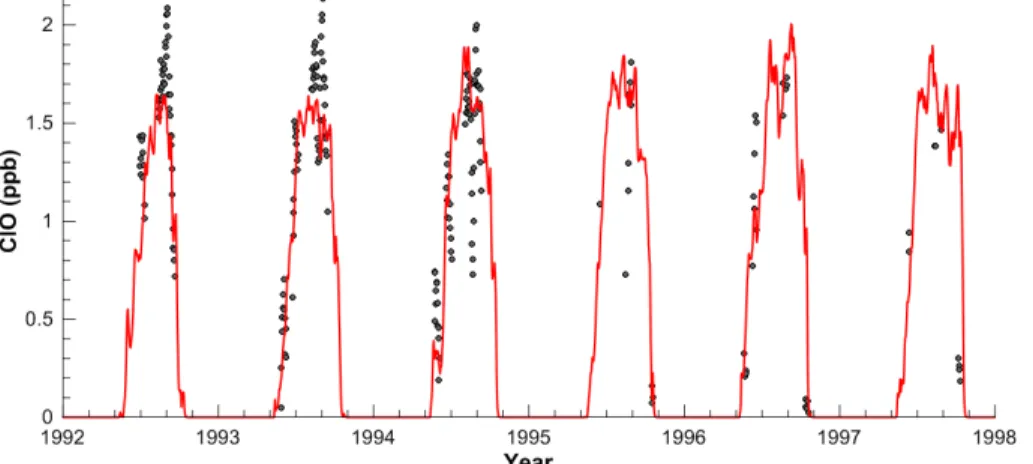
In Fig. 1 ClO observations and the semi-empirical model fit are shown. The model tracks the observations for activation and deactivation of ClO well. Because of the short data record, the ability of the model to track large inter-annual variability in chlo-10

rine activation is not immediately apparent. We are restricted to use UARS MLS ClO measurements for this study since measurements from the AURA satellite are only made in the later afternoon over Antarctica and our assumption that ClO is a good proxy for ClO_x does not apply in that case. Due to a known bias in the data (Livesey et al., 2003), the MLS ClO measurements show some deviation from zero before and 15

after the period of chlorine activation (not shown in Fig. 1). Therefore, the fitting of the model (Eq. 1) to the observations was restricted to 20 May to 20 October.

Equation (1) describes the activation and deactivation of ClOxon one pressure level. To derive the fit coefficients, ClO measurements at 520 K potential temperature were used for the fitting and FAP and FAS were calculated at 50 hPa which is the closest 20

pressure level to the 520 K potential temperature surface. Using CCM output on 10 pressure levels we found that in the region of largest contribution (150–70 hPa), the fit coe_fficients do not vary significantly with altitude. Assuming no altitude dependence in the fit coefficients is therefore unlikely to introduce large uncertainties into our calcula-tion of ClOx from FAP and FAS on any pressure level. Equation (1) is applied to FAP 25

(7)

ACPD

12, 28451–28466, 2012

OMD

P. E. Huck et al.

Title Page

Tables Figures

◭ ◮

Back Close

Full Screen / Esc

Discussion

P

a

per

|

Dis

cussion

P

a

per

|

Discussion

P

a

per

|

Discussio

n

P

a

per

|

(Bodeker et al., 2002), then only temperature fields are required to derive ClO_x time series.

3 Ozone depletion model

The second semi-empirical model describes the time rate of change of ozone mass deficit (OMD), a measure of springtime chemical ozone loss over Antarctica (Huck 5

et al., 2007). OMD is a bulk measure of the size and depth of the ozone hole with respect to 1980 values, and it is one of the common metrics used to describe inter-and intra-annual variations in Antarctic ozone depletion (e.g. WMO, 2007, 2011). An improved definition of OMD (Huck et al., 2007) is used in this study which is better able to capture the intra-seasonal evolution than the traditional definition (Uchino et al., 10

1999).

The time rate of change of OMD is described using another first order differential equation of the form:

dOMD dt =

h

A×sMAC2+B×sMAC

i

×(1−S)−C×OMD×Fact

−D×OMD×WP×

1− κ κ_max

(2) 15

The ozone model consists of three terms. The first term relates the time rate of change of OMD to active chlorine. The amount of ozone that can be depleted has both a linear and a quadratic dependence on the amount of activated chlorine (Jiang et al., 1996). The sunlit mass of activated chlorine (sMAC) in Eq. (2) is an estimate of the total mass 20

of activated chlorine in the atmospheric column relative to 1980 values and multiplied by FAS. The mass of activated chlorine (MAC) in the stratosphere is calculated for each layer as:

MAC=(ClOx−ClOx 1980)× MCl Mair

×A×∆p×1

g (3)

(8)

ACPD

12, 28451–28466, 2012

OMD

P. E. Huck et al.

Title Page

Tables Figures

◭ ◮

Back Close

Full Screen / Esc

Discussion

P

a

per

|

Dis

cussion

P

a

per

|

Discussion

P

a

per

|

Discussio

n

P

a

per

|

where ClO_x, obtained from Eq. (1), is the ClO_x mixing ratio between two pressure levels. ClOx 1980 is the background ClOx concentration corresponding to 1980 values. The time series for 1979–1981 were averaged to derive the concentration of active chlorine in 1980. The estimate for ClO_x in 1980 (ClO_{x 1980}) is calculated by fitting a six-term Fourier expansion to the 1979–1981 average ClOx time series on each pressure 5

level.MCl is the molecular mass of chlorine (35.45 g mol− 1

), andMair is the molecular mass of dry air (∼29 g mol−1_)._A_{is the area of the polar vortex in m}2_,

∆pis the pressure di_fference for each layer in Pa, and g is the gravitational acceleration (9.81 m s−2_).

Assuming a homogeneous distribution of ClOxover the polar vortex, MAC is multiplied by FAS to account for the fact that sunlight is needed for ozone destruction due to 10

chlorine. Summation of MAC×FAS over all pressure levels (200, 150, 100, 70, 50, 30, and 20 hPa) results in an estimate of the sunlit mass of activated chlorine (above 20 hPa and below 200 hPa the contribution to activated chlorine is close to zero). In Fig. 2 the contribution of each layer to sMAC is shown for 2000. It can be seen that the largest contributions come from pressures between 150 and 70 hPa. To account for saturation 15

in ozone depletion (once ozone is depleted it cannot be depleted again),S is set to OMD/OMD₁₅₀, where OMD₁₅₀is the value OMD would have if total ozone everywhere inside the vortex was 150 DU, which is approximately the vortex average value of total column ozone when all the lower stratospheric ozone is destroyed (Bodeker et al., 2002).

20

The second term relates the time rate of change in OMD to in-situ production of ozone (through the Chapman cycle). This in-situ production of ozone through Chap-man chemistry is approximated via a parametrisation of the the actinic flux by taking the cosine of the solar zenith angle, and the area within the polar vortex into account (Grooß et al., 2011). Fact is a proxy of the actinic flux available to photolyse O2 and 25

form O₃.

(9)

ACPD

12, 28451–28466, 2012

OMD

P. E. Huck et al.

Title Page

Tables Figures

◭ ◮

Back Close

Full Screen / Esc

Discussion

P

a

per

|

Dis

cussion

P

a

per

|

Discussion

P

a

per

|

Discussio

n

P

a

per

|

is the maximum of the meridional impermeability on each day, whileκmax is the max-imum of the meridional impermeability for all equivalent latitudes and days in a given year (Bodeker et al., 2002). The D term therefore quantifies the exchange of ozone between the interior and exterior of the vortex which is driven by wave mixing (hence the inclusion of the WP term) but blocked by the impermeability of the vortex (hence 5

the inclusion of theκ-based term).

A, B, C and D in Eq. (2) are fit coefficients derived by optimally fitting the equa-tion to OMD from observaequa-tions. Equaequa-tion (2) is also solved using a 4th order Runge– Kutta algorithm. The equation is fitted to OMD calculated from the observational NIWA (National Institute of Water and Atmospheric research) combined total column ozone 10

database (Bodeker et al., 2005) from 1990 to 2000. The fitting method used to find the optimal solution is the same parameter space grid search technique as used for the chlorine activation model (Eq. 1). The terms after each fit coefficient were normalised to vary between 0 and 1, to make the fit coe_fficients comparable to each other. They result inA=4.41×10−7,B=0.67,C=0.36, andD=1.43×10−2. Similar to the fit co-15

efficients in the chlorine model, no uncertainties are available with this fitting technique and the parameter values give the best fit to the data. The robustness of the fitting technique was tested by fitting to different periods and different number of years. The fit coefficientsAandDare small compared toB andC, which indicates that the linear dependence of ozone depletion on chlorine and the in-situ production are the critical 20

terms when describing the inter- and intra-annual variability of OMD. When the ozone depletion model is run from 1980 to 2010, the correlation coefficient between the model and observations isR2=0.97 over the entire period.

To test the predictive capability of the semi-empirical models, the dynamical variabil-ity term (Dterm) was excluded and the input parameters FAS and FAP (now the only 25

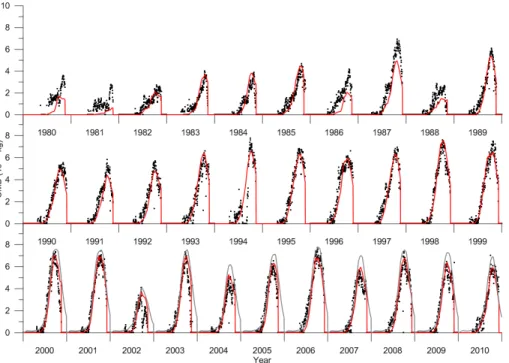
required parameters besides Cl_y) were calculated for 2000 to 2010 assuming a con-stant vortex edge at 62◦_{S (see also Huck et al., 2007). In Fig. 3 OMD observations,}

the full model, and the simplified model predictions are shown for 1980 to 2010. The model tracks the observations for the seasonal evolution of ozone depletion. The

(10)

ACPD

12, 28451–28466, 2012

OMD

P. E. Huck et al.

Title Page

Tables Figures

◭ ◮

Back Close

Full Screen / Esc

Discussion

P

a

per

|

Dis

cussion

P

a

per

|

Discussion

P

a

per

|

Discussio

n

P

a

per

|

to-year variability of the Antarctic ozone hole is also well represented, in particular for the anomalous years 1988, 2002 and 2004. The simulation using the simplified version of the model reproduces intra- and inter-annual variability of OMD. The fact that both model versions track the observations between 2000 and 2010 (including two of the anomalous years), which were not used to derive the fit parameters, demonstrates the 5

predictive capability of such semi-empirical models.

4 Discussion and conclusion

Fit coefficients such as those in the two semi-empirical models described above can be used to determine key sensitivities in the stratosphere. For example, the fit coefficients of the OMD model (Eq. 2) indicate a linear dependence between ozone depletion and 10

chlorine in the Antarctic stratosphere in agreement with the findings of Harris et al. (2010).

Activation of chlorine in the polar stratosphere in the future will be linked to climate change: future increases in atmospheric concentrations of GHGs will cool the strato-sphere which, together with possible increases in water vapor (WMO, 2011), will pro-15

mote the formation of PSCs. In contrast, likely increases in wave activity emanating from the troposphere into the stratosphere driven by changes in surface climate will warm the stratosphere. The future interplay between these factors is unknown (WMO, 2011). Fit coefficients of semi-empirical models such as those described above can be used to investigate aspects of the interaction between climate change and Antarctic 20

ozone depletion.

It was shown that a further simplification of the equations by excluding the dynami-cal variability term and by replacing the actual dynamidynami-cal vortex edge with the average location of the vortex edge of 62◦_{S provides models with the ability to project the}

devel-opment of Antarctic ozone into the future. As long as temperature projections and Cly 25

(11)

ACPD

12, 28451–28466, 2012

OMD

P. E. Huck et al.

Title Page

Tables Figures

◭ ◮

Back Close

Full Screen / Esc

Discussion

P

a

per

|

Dis

cussion

P

a

per

|

Discussion

P

a

per

|

Discussio

n

P

a

per

|

example, be used to produce an ensemble of ozone projections considering a range of GHG emissions scenarios.

There are limitations to these equations, which is why this study should be consid-ered as proof-of-concept rather than a finished product. As they stand, these semi-empirical models cannot be applied outside the Antarctic vortex. Finer di_fferentiation 5

between physical and chemical processes might be necessary for more detailed stud-ies of key atmospheric sensitivitstud-ies of ozone depletion and climate change. These semi-empirical models which only consider bulk quantities do not appear to be very sensitive to changes in atmospheric dynamics. Due to the expected increase in the importance of dynamical processes, it might be necessary to model single levels in the atmosphere 10

in the future.

Acknowledgements. This work was supported by the DFG (Deutsche Forschungsgemein-schaft) and by the Marsden Fund Council from Government funding, administered by the Royal Society of New Zealand. NCEP/NCAR reanalyses were provided by the NOAA-CIRES Climate Diagnostics Center, Boulder, Colorado, USA, from their Web site at http://www.cdc.noaa.gov/.

15

We would like to thank Michelle Santee for providing the MLS data and for detailed comments and suggestions on the manuscript.

References

Bodeker, G. E., Struthers, H., and Connor, B. J.: Dynamical containment of Antarctic ozone depletion, Geophys. Res. Lett., 29, 1098, doi:10.1029/2001GL014206, 2002. 28457, 28458,

20

28459

Bodeker, G. E., Shiona, H., and Eskes, H.: Indicators of Antarctic ozone depletion, Atmos. Chem. Phys., 5, 2603–2615, doi:10.5194/acp-5-2603-2005, 2005. 28459

Brasseur, G. and Solomon, S.: Aeronomy of the Middle Atmosphere, Springer, Dordrecht, The Netherlands, 2005. 28454

25

Cariolle, D. and Teyss `edre, H.: A revised linear ozone photochemistry parameterization for use in transport and general circulation models: multi-annual simulations, Atmos. Chem. Phys., 7, 2183–2196, doi:10.5194/acp-7-2183-2007, 2007. 28453

(12)

ACPD

12, 28451–28466, 2012

OMD

P. E. Huck et al.

Title Page

Tables Figures

◭ ◮

Back Close

Full Screen / Esc

Discussion

P

a

per

|

Dis

cussion

P

a

per

|

Discussion

P

a

per

|

Discussio

n

P

a

per

|

Chapman, S.: A theory of upper atmospheric ozone, Mem. Roy. Soc., 3, 103–109, 1930. 28453 Charlton-Perez, A. J., Hawkins, E., Eyring, V., Cionni, I., Bodeker, G. E., Kinnison, D. E., Akiyoshi, H., Frith, S. M., Garcia, R., Gettelman, A., Lamarque, J. F., Nakamura, T., Paw-son, S., Yamashita, Y., Bekki, S., Braesicke, P., Chipperfield, M. P., Dhomse, S., Marc-hand, M., Mancini, E., Morgenstern, O., Pitari, G., Plummer, D., Pyle, J. A., Rozanov, E.,

5

Scinocca, J., Shibata, K., Shepherd, T. G., Tian, W., and Waugh, D. W.: The potential to nar-row uncertainty in projections of stratospheric ozone over the 21st century, Atmos. Chem. Phys., 10, 9473–9486, doi:10.5194/acp-10-9473-2010, 2010. 28452, 28453

Chipperfield, M. P. and Pyle, J. A.: Model sensitivity studies of Arctic ozone depletion, J. Geo-phys. Res.-Atmos., 103, 28389–28403, 1998. 28454

10

Grooß, J.-U., Brautzsch, K., Pommrich, R., Solomon, S., and M ¨uller, R.: Stratospheric ozone chemistry in the Antarctic: what determines the lowest ozone values reached and their re-covery?, Atmos. Chem. Phys., 11, 12217–12226, doi:10.5194/acp-11-12217-2011, 2011. 28454, 28458

Harris, N. R. P., Lehmann, R., Rex, M., and von der Gathen, P.: A closer look at Arctic ozone

15

loss and polar stratospheric clouds, Atmos. Chem. Phys., 10, 8499–8510, doi:10.5194/acp-10-8499-2010, 2010. 28460

Hsu, J. and Prather, M. J.: Stratospheric variability and tropospheric ozone, J. Geophys. Res.-Atmos., 114, D06102, doi:10.1029/2008JD010942, 2009. 28453

Huck, P. E., McDonald, A. J., Bodeker, G. E., and Struthers, H.: Interannual variability in

Antarc-20

tic ozone depletion controlled by planetary waves and polar temperature, Geophys. Res. Lett., 32, L13819, doi:10.1029/2005GL022943, 2005. 28458

Huck, P. E., Tilmes, S., Bodeker, G., Randel, W., McDonald, A., and Nakajima, H.: An improved measure of ozone depletion in the Antarctic stratosphere, J. Geophys. Res., 112, D11104, doi:10.1029/2006JD007860, 2007. 28457, 28459

25

Jiang, Y. B., Yung, Y. L., and Zurek, R. W.: Decadal evolution of the Antarctic ozone hole, J. Geophys. Res.-Atmos., 101, 8985–8999, 1996. 28457

Livesey, N. J., Read, W. G., Froidevaux, L., Waters, J. W., Santee, M. L., Pumphrey, C. H., Wu, D. L., and Jarnot, R. F.: The UARS Microwave Limb Sounder version 5 data set: theory, characterization, and validation, J. Geophys. Res., 108, D134378,

30

(13)

ACPD

12, 28451–28466, 2012

OMD

P. E. Huck et al.

Title Page

Tables Figures

◭ ◮

Back Close

Full Screen / Esc

Discussion

P

a

per

|

Dis

cussion

P

a

per

|

Discussion

P

a

per

|

Discussio

n

P

a

per

|

McLinden, C., Olsen, S., Hannegan, B., Wild, O., and Prather, M.: Stratospheric ozone in 3-D models: a simple chemistry and the cross-tropopause flux, J. Geophys. Res., 105, 14653– 14665, 2000. 28453

Newman, P. A., Nash, E. R., Kawa, S. R., Montzka, S. A., and Schauffler, S. M.: When will the Antarctic ozone hole recover?, Geophys. Res. Lett., 33, L12814,

5

doi:10.1029/2005GL025232, 2006. 28454

Santee, M. L., Manney, G. L., Waters, J. W., and Livesey, N. J.: Variations and climatology of ClO in the polar lower stratosphere from UARS Microwave Limb Sounder measurements, J. Geophys. Res.-Atmos., 108, 4454, doi:10.1029/2002JD003335, 2003. 28456

Sinnhuber, B.-M., Sheode, N., Sinnhuber, M., Chipperfield, M. P., and Feng, W.: The

contri-10

bution of anthropogenic bromine emissions to past stratospheric ozone trends: a modelling study, Atmos. Chem. Phys., 9, 2863–2871, doi:10.5194/acp-9-2863-2009, 2009. 28454 Solomon, S.: Stratospheric ozone depletion: a review of concepts and history, Rev. Geophys.,

37, 275–316, doi:10.1029/1999RG900008, 1999. 28453

SPARC CCMVal: SPARC Report on the Evaluation of Chemistry-Climate Models, WCRP-132,

15

SPARC Report No. 5, Toronto, Canada, 2010. 28453

Uchino, O., Bojkov, R. D., Balis, D. S., Akagi, K., Hayashi, M., and Kajihara, R.: Essential char-acteristics of the Antarctic-spring ozone decline: update to 1998, Geophys. Res. Lett., 26, 1377–1380, 1999. 28457

von Hobe, M., Grooß, J.-U., M ¨uller, R., Hrechanyy, S., Winkler, U., and Stroh, F.: A re-evaluation

20

of the ClO/Cl₂O₂ equilibrium constant based on stratospheric in-situ observations, Atmos. Chem. Phys., 5, 693–702, doi:10.5194/acp-5-693-2005, 2005. 28454

Waugh, D. W. and Randel, W. J.: Climatology of Arctic and Antarctic polar vortices using ellip-tical diagnostics, J. Atmos. Sci., 56, 1594–1613, 1999. 28454

WMO: Scientific Assessment of Ozone Depletion: 2002, World Meteorological Organisation

25

Global Ozone Research and Monitoring Project Report No. 47, Geneva, Switzerland, 2003. 28454

WMO: Scientific Assessment of Ozone Depletion: 2006, World Meteorological Organization Global Ozone Research and Monitoring Project Report No. 50, Geneva, 2007. 28457 WMO: Scientific Assessment of Ozone Depletion: 2010, World Meteorological Organization

30

Global Ozone Research and Monitoring Project Report No. 52, Geneva, 2011. 28454, 28457, 28460

(14)

ACPD

12, 28451–28466, 2012

OMD

P. E. Huck et al.

Title Page

Tables Figures

◭ ◮

Back Close

Full Screen / Esc

Discussion

P

a

per

|

Dis

cussion

P

a

per

|

Discussion

P

a

per

|

Discussio

n

P

a

per

|

(15)

ACPD

12, 28451–28466, 2012

OMD

P. E. Huck et al.

Title Page

Tables Figures

◭ ◮

Back Close

Full Screen / Esc

Discussion

P

a

per

|

Dis

cussion

P

a

per

|

Discussion

P

a

per

|

Discussio

n

P

a

per

|

Fig. 2.Contribution from di_fferent atmospheric layers (as indicated in the legend) to the sun-lit mass of activated chlorine for the year 2000. Largest contributions come from pressures between 150–70 hPa.

(16)

ACPD

12, 28451–28466, 2012

OMD

P. E. Huck et al.

Title Page

Tables Figures

◭ ◮

Back Close

Full Screen / Esc

Discussion

P

a

per

|

Dis

cussion

P

a

per

|

Discussion

P

a

per

|

Discussio

n

P

a

per

|