FEEDFORWARD INS AIDING: AN INVESTIGATION OF MANEUVERS FOR
IN-FLIGHT ALIGNMENT
Jacques Waldmann
∗Department of Systems and Control - Instituto Tecnológico de Aeronáutica 12228-900 - São José dos Campos - SP - Brasil - (0xx12)39475993
RESUMO
Navegação em veículos autônomos requer a integração de medidas de sensores inerciais embarcados e informação externa adicional coletada por vários sensores. Neste artigo, o modelo de erro de velocidade representado no sistema de coordenadas computado é aumentado com um modelo de constante aleatória para descrever o erro de zero dos acelerômetros e girômetros. Essa modelagem visa à fusão de um sistema girante de navegação inercial de baixo custo com medidas externas de posição e velocidade empregando o filtro de Kalman. É investigado o impacto do erro de modelo e das manobras na estimação do desalinhamento e dos erros da unidade de medidas inerciais. Este trabalho simula os três canais de um sistema inercial de navegação, sem amortecimento vertical e dotado de unidade de medidas inerciais girante em relação ao veículo. A rotação da unidade de medidas inerciais não requer o mecanismo sofisticado típico de uma plataforma estabilizada mecanicamente, além de dispensar manobras que podem levar o veículo a se afastar da trajetória desejada e que são usualmente empregadas no alinhamento em vôo de plataformas solidárias ao corpo do veículo. Em comparação com a plataforma estabilizada mecanicamente e estacionária em local conhecido, a rotação da unidade de medidas inerciais melhora a estimação dos erros de zero dos acelerômetros e parcialmente melhora a estimação dos erros de zero dos girômetros e do desalinhamento. Finalmente, a combinação de rotação
Artigo submetido em 09/12/2004 1a. Revisão em 02/05/2006 2a. Revisão em 06/05/2007
Aceito sob recomendação do Editor Associado Prof. Liu Hsu
da unidade de medidas inerciais com segmentos distintos de aceleração produz observabilidade completa, resultando assim em melhoria significativa nas estimativas dos erros de zero dos girômetros e do desalinhamento.
PALAVRAS-CHAVE: navegação inercial, alinhamento em vôo, fusão de sensores, veículos autônomos, robótica.
ABSTRACT
of accelerometer bias, and partially improves estimation of rate-gyro drift and misalignment. Finally, combining IMU rotation with distinct acceleration segments yields full observability, thus significantly enhancing estimation of rate-gyro drift and misalignment.
KEYWORDS: inertial navigation, in-flight alignment, sensor fusion, autonomous vehicles, robotics.
GLOSSARY
DCM – direction cosine matrix.
GINS – mechanically stabilized, gimbaled–based INS.
IFA – in-flight alignment.
IMU – inertial measurement unit.
INS – inertial navigation system.
NED – North-East-Down.
PWC – piece-wise constant.
SDINS – strapdown inertial navigation system.
SOM – stripped observability matrix.
WGS-84 – World Geodetic System 1984 geoid-interpolating geocentric reference ellipsoid.
x
A– time derivative of vectorAas computed by an observer
attached to reference frame Sx.
x A
y– representation of x
Ain reference frame Sy.
Asp– specific force sensed by accelerometer triad.
Dxy– DCM from reference frame Sxto Sy.
gm, g– Earth’s gravitation and gravity, respectively.
g0– WGS–84 Earth’s equatorial gravity magnitude.
h – altitude above WGS–84 ellipsoid.
R– true position.
RN, RE – WGS–84 latitude-dependent northward and eastward Earth’s curvature radii, respectively.
Re– WGS–84 latitude-dependent Earth’s radius.
R0– WGS–84 Earth’s equatorial radius.
Ss– navigation reference frame.
Sx– x-reference frame, x={b,c,e,i,NED,p,s,t}.
Ve– terrestrial velocity, equal to
e
R.
λ,Λ– geographic latitude and longitude, respectively.
∆R– position error.
∆Ve– terrestrial velocity error.
ε– rate-gyro drift.
ρ– transport rate vector, equal toωse.
ω–Inertial angular rate vector of Ss, equal toωsi.
ωxy– angular rate of S
xrelative to Sy.
Ω– Earth’s inertial angular rate, equal toωei.
Ωxyx – skew-symmetric matrix representation of vector cross-product operator [ωxxy×](.).
δθ– Misalignment vector from Stto Sc.
ψ– Misalignment vector from Scto Sp.
φ– Misalignment vector from Stto Sp.
∇– accelerometer bias.
Subscripts:
a – aiding sensor external to INS.
b – IMU reference frame.
c – computer reference frame.
e – Earth-fixed reference frame.
i – inertial reference frame.
m – measured quantity.
p – platform reference frame.
s – navigation reference frame.
t – true reference frame.
0 – initial value.
1
INTRODUCTION
and rate-gyros capable of measuring specific force and angular rate components. Gimbaled INS implementations (GINS) employ accurate mechanisms to isolate the IMU from the host vehicle’s motion and keep alignment with the navigation reference frame. A strapdown configuration (SDINS) employs an IMU rigidly attached to the host vehicle. IMU sensors often provide signals in discrete time and incremental form, and adequate numerical integration provides the desired estimates. The INS can track short-term, abrupt motions, but estimation errors grow unbounded during long operation periods due to the integration of low-frequency errors such as accelerometer bias and rate-gyro drift, which are unknown, constant null offsets.
Before entering navigation mode, IMU calibration and alignment – often relative to the North-East-Down frame – make use of leveling and gyrocompassing, which are based on reaction to gravity and earth rate sensing while the vehicle remains stationary at a known location on the ground. However, some circumstances demand in-flight alignment (IFA) (Baziw and Leondes, 1972). More recently, autonomous vehicles often resort to a low-cost SDINS aided by additional sensors, and Kalman filter-based sensor fusion is employed to estimate navigation, misalignment and IMU errors (Adam et al., 1999; Roumeliotis et al., 2002; Eck and Geering, 2000; Hafskjold et al., 2000, and Wagner et al., 2003). Sequential Monte Carlo methods, particle filters, and other nonlinear estimators have also been investigated (Nordlund, 2000; Vik et al., 2001; Wan et.al., 2001).
Bar-Itzhack and Berman (1988) showed the lack of full observability when estimating misalignment and IMU errors of a stationary GINS with velocity error measurements. Their analysis employed linear navigation and misalignment error dynamics augmented with random constant accelerometer bias and rate-gyro drift. Goshen-Meskin and Bar-Itzhack (1990) departed from the augmented computer-frame velocity error model of a GINS, investigated its observability, and indicated that the ability to maneuver is “a blessing in disguise”. That is, though IFA may seem to be less accurate and more complicated than alignment at rest, maneuvers during the IFA phase can excite latent modes. Acceleration maneuvers in a GINS were modeled by a concatenation of piece-wise constant (PWC) specific force segments to circumvent the trajectory-dependent, numerical computation of the observability Grammian of a linear time-varying model. Observability analysis of the PWC linear error dynamics was based on determining the rank of the stripped observability matrix (SOM) after each acceleration segment (Goshen-Meskin and Bar-Itzhack, 1990; Leeet al.,
1993). The SOM analysis disregarded the actual model mismatch arising from linearization errors during operation and its effect on error estimation accuracy.
Rotorcraft and aerial vehicles with vectorized thrust are capable of PWC acceleration segments without significant attitude maneuvers. Goshen-Meskin and Bar-Itzhack (1990) claimed that covariance simulation and real IFA results showed that the exact nature of acceleration maneuvers is not influential, but their mere existence is paramount for accurate GINS misalignment and IMU error estimation. Thus, insights from SOM analysis apply to other GINS-equipped vehicles and maneuvers. On the other hand, SDINS-equipped vehicles without vectorized thrust must conduct attitude maneuvers to generate accelerations. It is intuitive that maneuvers in acceleration and IMU attitude should enhance estimation accuracy, but continuously changing IMU attitude violates the assumption of PWC dynamics, which precludes SOM analysis.
The purpose of this investigation is to gauge the impact of IMU rotation and PWC acceleration segments on estimation accuracy relative to a GINS undergoing the same acceleration maneuvers. Optimal maneuver design for IFA
is not within the scope of this work. Instead of a strapdown configuration, the IMU rotates relative to the host vehicle.
Hence, the host vehicle need not maneuver away from the desired path during the IFA phase. Following the IFA phase, the IMU can be locked in a known attitude relative to the vehicle. IMU rotation does not require the accurate mechanism of a gimbaled INS because what matters is to change the direction of the inertial sensors’ sensitive axes relative to gravity and earth angular rate. The approach has been inspired by Lee et al. (1993), which employed
SOM analysis and concatenated PWC segments of IMU attitude for multiposition alignment on the ground. Notice that vehicle attitude is a by-product of the conventional strapdown configuration at all times, whereas during IFA phase the present approach produces IMU attitude. The inertial sensors are assumed to be aligned with the IMU frame Sb.
Section 2 presents the navigation and attitude equations, and the multirate algorithm. Section 3 shows the computer-frame velocity error model for use in the Kalman filter. Section 4 discusses sensor fusion by means of indirect, feedforward INS-aiding with position and velocity measurements. Section 5 presents the simulation of stationary and IFA phase of both GINS and rotating IMU configurations, and analyzes the results, and conclusions are in Section 6.
2
THE NAVIGATION EQUATIONS
constant inertial earth rate ωei = Ω of S
e relative to Si, and the inertial rateωsi = ω of S
s relative to Si. Thus,
ωse=ρ=ω−Ωis the transport rate. LetRdenote position and the superscript indicate the coordinate frame in which a time derivative is observed. Neglecting measurement errors, accelerometers provide the specific force:
Asp=
ii
R−gm, (1)
wheregm=gm(R) is the gravitational pull toward the earth center due to mass attraction, andRii is the inertial second
derivative, i.e., inertial acceleration. Inertial velocity is:
i
R=Re +Ω×R=Ve+Ω×R, (2)
andVe is the terrestrial velocity observed from the earth-fixed coordinate frame Se. From (2), inertial acceleration is given by:
ii
R=Vie+Ω×
i
R=Vie+Ω×(Ve+Ω×R). (3)
It is desirable to describeVse= se
R, i.e., the rate of terrestrial
velocity as observed in the navigation frame Ss. Since i
Ve =
s
Ve+ωsi×Ve, (3) yields:
ii
R=
s
Ve+(ω+Ω)×Ve+Ω×(Ω×R). (4)
Substitution in (1) and rearranging gives:
s
Ve=Asp−(ω+Ω)×Ve+g, g=−Ω×(Ω×R) +gm, (5a)
whereg=g(R) is the local plumb-bob gravity vector. The
corresponding terrestrial position rate as observed in Ssis:
s
R=Ve−ρ×R. (5b)
Equations (5a-b) are the navigation vector equations. Specific force measurements, a gravity model, and knowledge of initial conditionsVe(0) andR(0) are needed to obtain the inertial estimatesVe,INS(t) andRINS(t). Equations (5a-b) are often mechanized to reflect the choice of Ss≡SN ED. The U.S. Department of Defense World Geodetic System (DoD WGS-84) approximates the earth’s
shape by a geocentric reference ellipsoid, which models earth radius Re, curvature radii RE and RN along East and North directions, respectively, and gravity (Siouris, 1993). Latitudeλ, longitudeΛ, and altitude h describe the terrestrial position. The vertically-undamped, continuous-time navigation equations are:
˙
λ= VN
RN+h ,
˙Λ = VE
(RE+h) cos(λ) ,
˙
h=−VD,
˙
VN =Asp,N+
VNVD
(RN +h)
−VE{2Ωsin(λ) +
VEtan(λ)
(RE+h) },
˙
VE =Asp,E+VN{2Ω sin(λ) +
VEtan(λ) (RE+h)}+ +VD{2Ω cos(λ) +(RVE
E+h)},
˙
VD=Asp,D−
VNVN
(RN+h)
−VE{2Ω cos(λ) + VE
(RE+h) }+
+g(λ, h). (6)
whereg(λ, h) = g0(1 + 0.0053sin2(λ))(1−2h/R
e)is a sufficiently accurate approximation of gravity. Inaccurate knowledge about gravity is not among the most significant sources of errors in stand-alone, low-cost INS operation where the effect of IMU errors strongly exceed those due to gravity errors (Jekeli, 1997). Use of accelerometer data in (6) needs attitude determination, i.e. the transformation from Sb to SN ED according toAsp,NED =DbNED,INSAsp,b,m. One approach is to compute the direction cosine matrix (DCM) from angular rate measurements and the initial alignment
DbNED,INS(0):
˙
DbNED,INS=D b NED,INSΩ
bi b,m−Ω
NEDi NED,INSD
b
NED,INS. (7)
The entries in skew-symmetric (cross product form) matrix
Ωbi
b,m are the components of the angular rate sensed by the IMU’s rate-gyro triad. Likewise, skew symmetric matrix
ΩNEDi
ωNEDi NED,INS=ω
ei
NED,INS+ω NEDe NED,INS=
=ΩNED,INS+ρNED,INS=
=
ΩN,IN S
0 ΩD,IN S
+
ρN,IN S ρE,IN S ρD,IN S
=
=
(Ω + ˙ΛIN S) cos(λIN S) −λ˙IN S
−(Ω + ˙ΛIN S) sin(λIN S)
, (8)
where ˙ΛIN S,λ˙IN S, λIN S are from the INS stand-alone solution to (6).
The INS stand-alone solution to (6) and (7) is computed by a multirate algorithm that processes IMU discrete-time measurements, that is angular and thrust velocity increments occurring between sensor samples (Bar-Itzhack, 1978; Savage, 1998; Waldmann, 2003). Coning errors arise because finite rotations do not commute, sculling errors are due to incorrect thrust velocity computation as coordinate frames rotate between data samples, and scrolling errors arise from velocity and position updates occurring at distinct rates. Though complex, with intricate compensation terms to attenuate such errors, Savage’s multirate approach has been utilized due to its accuracy. Thrust velocity increments from the accelerometers are transformed from Sb to SN ED at a high sampling rate, and terrestrial velocity and position are solved at intermediate and slow rates, respectively. The fast acquisition rate of incremental inertial samples and attitude computation has been set to 400Hz. The INS terrestrial velocity and position are computed at the intermediate and slow rates 1/Tint=200Hz and 1/Tnav=100Hz, respectively. The stand-alone inertial solution diverges due to errors in IMU data and erroneous processing by the multirate algorithm, thus causing linearization errors and model mismatch in the Kalman filter.
3
THE
COMPUTER-FRAME
VELOCITY
ERROR MODEL
Figure 1 shows the most relevant NED coordinate frames and misalignment angles for a brief description of this error model. True, computed, and platform frames, St, Sc, and Sp, respectively, are located at the actual and estimated positions. Sc is perfectly known, albeit it is incorrect. If initial alignment and inertial data were error free, the integration of (7) would produceDbt. However, accelerometer bias and
rate-gyro drift yieldDbp=DbNED,INS.
δθis a small misalignment angle vector due to errors in the estimated position.δθrotates Stinto alignment with Sc, and
Figure 1: NED coordinate frames and misalignment angles
is represented in Scas:
δθc=
∆RE/(RE(λ) +h) −∆RN/(RN(λ) +h) −∆REtan(λ)/(RE(λ) +h)
, (9)
where REand RN are the earth’s curvature radii, and∆RE and ∆RN are position errors. The small misalignment angle vectorψ is due to rate-gyro drift, and rotates Sc into alignment with Sp. Use of the computer frame Sc for the error model is attractive because it renders the misalignment rateψc uncoupled from both position and terrestrial velocity
errors. The total misalignment angleφ=δθ+ψfrom Stto Sp can be estimated from (9) using the INS solution to (6), and the Kalman filter estimates ofψand∆R.
Assuming a spherical earth and the IMU path in the vicinity of the earth’s surface (i.e. h«R0 and |R| ≈R0),
the computer-frame position error model was obtained and further elaborated to show its equivalence to the computer-frame velocity error model (Waldmann, 2004). The latter describes the error dynamics with a structure
•
∆x’NED =
A′(t)∆x′
∆x′ NED=
∆RTNED ∆V
T
e,NED ψ
T
NED
T,
∆u= ∇T
b ε
T
b
T
,
∆RNED= ∆RN ∆RE ∆RD T
,
∆Ve,NED=
∆VN ∆VE ∆VD T
,
ψNED= ψN ψE ψD T
,
∇b= ∇Xb ∇Y b ∇Zb
T ,εb=
εXb εY b εZb T
,
A′=
A11 I3 03
A21 A22 A23
03 03 A33
,
A11=
0 ρD −ρE
−ρD 0 ρN
ρE −ρN 0
,
A21=diag(−g0/R0,−g0/R0,2g0/R0),
A22=
0 ρD+ 2ΩD −ρE −(ρD+ 2ΩD) 0 ρN + 2ΩN
ρE −(ρN+ 2ΩN) 0
,
A23=
0 −Asp,D Asp,E
Asp,D 0 −Asp,N
−Asp,E Asp,N 0
,
B=
03x3 03x3
Db
p 03x3
03x3 −Dbp
,
A33=
0 ρD+ ΩD −ρE −(ρD+ ΩD) 0 ρN + ΩN
ρE −(ρN + ΩN) 0
.
(10)
To estimate the IMU errors, assuming full observability, the above error vector was augmented with a random constant model of accelerometer bias∇b and rate-gyro driftεb. The augmented dynamics is∆x• = A(t)∆x+n, with n white
noise, and∆x∈R15:
∆x= ∆x′ NED ∆u
, A=
A′ B
06x9 06
. (11)
4
INDIRECT FEEDFORWARD INS AIDING
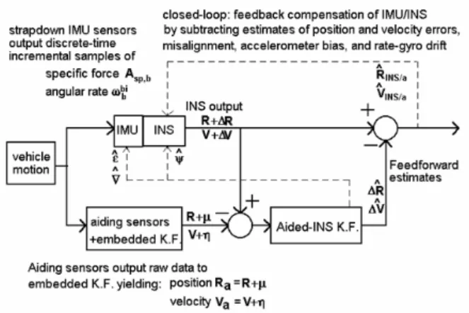
The continuous lines in Figure 2 depict a feedfoward, indirect Kalman filter-based fusion of INS estimates with aiding position and terrestrial velocity. The aiding signals result from the processing of observables within the aiding sensors. The latter may be a GPS receiver, or a camera trained on a
known landmark. The term "indirect" refers to error state estimation rather than estimation of the full state. The dashed lines in Figure 2 indicate INS reset by feeding back estimates of misalignment and IMU error, i.e. accelerometer bias and rate-gyro drift.
Noting that subscript a indicates aiding sensor, and measurement y is the difference between the INS solution
and the aiding position and velocity, then:
RINS=R+ ∆R, Ve,INS=Ve+ ∆Ve, (12)
y=
RINS−Ra
Ve,INS−Ve,a
=
∆R−µ
∆Ve−η
. (13)
Representation of the above aiding differences in the NED coordinate frame yields:
∆RN = (λIN S−λa)(RN +ha),
∆RE= (ΛIN S−Λa)(RE+ha) cos(λa),
∆RD=−(hIN S−ha),
∆Ve,NED=
= (Ve,INS−Ve,a)NED=
∆VN ∆VE ∆VD
T
. (14)
Ideally,µandηin Figure 2 are white and uncorrelated noise processes. However, the processing of observables gives rise to correlation in time and among components of aiding position and velocity. Such correlations are not considered here in the statistical model of measurement errors. Thus, the discrete-time measurement equation in the aided-INS Kalman filter is yj = [∆RNED(j)T∆Ve,NED(j)T]T =
H∆xj+vj, wherevj is a zero-mean, white sequence with diagonal covarianceR¯, andH= diag(I6,O6x9).
The INS solution-dependent parameters Asp, Ve,INS, RINS andDbpin (11) have been updated at rate 1/Tnav=100Hz.A(t) has been discretized to produce the state transition matrix, that is Φk = I+A(kTnav)Tnav(I+A(kTnav)Tnav/2). Uncertainty inΦk has been translated into an additive, zero-mean, white noise sequence wk with diagonal covariance matrixQ, which is related to the linearization error about the
diverging INS solution.Qdemanded tuning. Filter estimates
Figure 2: Indirect feedforward INS-aiding architecture.Vis
herein used to denote the terrestrial velocityVe.
of the estimation error. The Kalman filter equations and corresponding computation rates are:
Initialization:
∧ ∆x+0 =
∧
∆x0 ;P+0 =P0; k=0 ; j=1;
Propagation until update available – 1/Tnav=100Hz:
k=k+1;
∧
∆x−k = Φk−1 ∧ ∆x−k−1;
P−k = Φk−1P−k−1Φ
T
k−1+Q;
Update available – 1/Ta=1Hz:
∧ ∆x−j =
∧
∆x−k ;P−j =P−k;
Kj =P
−
jH
T[HP−
j H
T +R¯]−1;
∧ ∆x+j =
∧
∆x−j +Kj[yj−H
∧
∆x−j]; k=0 ;
∧ ∆x−k =
∧ ∆x+j;
P+j = [I15−KjH]P
−
j ;P
−
k =P
+
j ; j=j+1.
Return to propagation stage.
¯
R=diag((3[m])2I3,(0.05[m / s])2I3),
P0=diag((10[m])2I3,(0.5[m / s])2I3,Z,
(3I3∇b[m / s2])2,(3I3εb[rd / s])2),
Z=diag((∇E/ g[rd])2,(∇N/g[rd])2,
((−εE+ ΩD0∇E/ g)/ΩN0[rd])2),
h
∇T
NED εNED
TiT
=diag(Db p,D
b p)
∇T
b εTb
T
,
Q=Tnav.diag((1[m])2I3,(10
−5
[m / s])2I3,01x9).
P0 mirrored the initial uncertainty in the estimation error.
The diagonal form of Z represents the impact of IMU
errors ∇NED and εNED on the uncertainty about initial misalignment angleψNED(0).
Due to model mismatch, the residual sequencerj = yj −
H
∧
∆x−j at instants multiple of Ta has been monitored to ensure statistical consistency (Bar-Shalom and Li, 1993). Adequate tuning ofQshould produce a zero-mean, white,
Gaussian residual sequence with covariance matrix Sj = HP−j HT + R¯. Had a position or velocity residual
component been found outside ±3 times the square root of the corresponding element in the diagonal of S, the
corresponding position or velocity error variance in P
was reset to (3m)2 and (0.3m/s)2, respectively. The
corresponding off-diagonal elements inPwere also altered
to keep the cross-correlation coefficients unchanged by the reset.
5
MANEUVERS AND RESULTS
Goshen-Meskin and Bar-Itzhack (1990) modeled maneuvers during the IFA phase of a GINS with 20 seconds, PWC, 0.1g specific force segments. Consequently,Dbp = I, and A23
in (11) was the single PWC, significantly time-varying block inA(t). IMU rotation, however, violates conditions for valid
SOM analysis becauseDb
pinB(t) varies continuously. The
impact of PWC acceleration segments and IMU rotation on estimation accuracy,both at a known location on the ground and during IFA, is gauged with the filter-computed standard
deviation of the estimation error and, as in Pittelkau (2005), one realization.
Aiding position and velocity measurements, respectively
Ra and Ve,a, have been generated from ground-truth corrupted by additive Gaussian, zero-mean, white noise with covariance matrix R¯. IMU rotation with respect to the
vehicle has been simulated with IMU attitude ground-truth in terms of yaw, pitch, and roll relative to the NED coordinate frame (Bar-Itzhack, 1977):
ψ=s(2πt/300) + 0.5s(2πt/1.7)[rd],
θ=s(2πt/300) + 0.5s(2πt/1.7 + 0.3)[rd], φ=s(2πt/300) + 0.5s(2πt/0.85)[rd], t∈[0,200][s].
(15)
The GINS stand-alone solution was simulated by enforcing thatψ ≡θ ≡φ ≡0, generating IMU data, and solving (6) and (7). In this case of NED mechanization,Db
p = Iand
Xb ≡ N, Yb ≡ E, andZb ≡ D. Each rate-gyro has
zero-mean, white noise with standard deviationσε=1˚/h, and integrated between consecutive sensor samples to yield the incremental angular measurements.
Given the initial position and terrestrial velocity, and ground acceleration V˙N,V˙E,V˙D which the IMU was subject to,
the NED ground-truth specific force Asp,t was obtained
from (6). From (15), Dt
bAsp,t was computed, and each
accelerometer corrupted by bias∇Xb =∇Y b =∇Zb=3mg and additive zero-mean, white noise with standard deviation σ∇=1mg. Integration between consecutive sensor samples
resulted in the incremental thrust velocity measurements.
Motion 1 aimed to show whether a constant, long-duration acceleration can enhance observability, though its ultimate velocity is surely not attainable by a low-cost host vehicle. With λ(0)=23˚12′S,Λ(0)=45˚52′W, and h(0)=600m as the initial location at ITA facilities, Motion 1 consisted of constant ground acceleration a=5m/s2(Bar-Itzhack, 1977):
VN =VE=−VD= 300 +at[m/s],t∈[0,200][s]. (16)
With the same initial location and terrestrial velocity, Motion 2 comprised five PWC, 40s ground acceleration segments as in Table 1.
Segment V˙N V˙E V˙D
1 0 0 0
2 a 0 0
3 0 a 0
4 a a 0
5 0 0 -a
Table 1: Motion 2 ground acceleration segments
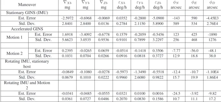
Table 2 summarizes the effect of the maneuvers on one realization of the estimation error of IMU sensor errors and misalignment at t=200s, and respective filter-computed standard deviation. Figures 4-6 show the ±1-sigma filter-computed standard deviation of the estimation error (i.e. filter uncertainty) and one realization of the estimation error for Motion 2 combined with IMU rotation.
5.1
Stationary GINS at a known location
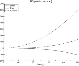
In this case, from (6) one hasAsp,NED = −g(λ(0), h(0))D because Ve = 0. The position error of the stand-alone INS is in Figure 3. INS-aided position estimation error in Figure 4 shows that sensor fusion has sucessfully damped the instability inherent to the INS vertical channel. Other
0 40 80 120 160 200 -200
-100 0 100 200 300 400 500 600 700
Time [s]
INS position error [m]
North East Altitude
Figure 3: Stationary GINS true position error (m)
results shown in Table 2 are briefly analyzed in the ensuing due to lack of space. The information content available in this condition only partially reduced the initial filter uncertainty about biases in the horizontal accelerometers. Vertical accelerometer (Zb) bias, however, was accurately estimated.
Filter uncertainty about drift in the Xb horizontal rate-gyro was reduced more significantly than in the Yb channel. Filter-computed standard deviation of vertical Zb rate-gyro drift and azimuth misalignment estimation error confirmed a lack of observability which is consistent with Bar-Itzhack and Berman (1988). Similar results have been observed in the case of a GINS whose IMU displaced with constant ground velocityVN =VE =−VD = 300m/sbecause the horizontal specific force was negligible (see (6)).
5.2
GINS undergoing acceleration
Motion 1 reduced filter uncertainty with respect to drift in the vertical (Zb) and horizontal (Yb) gyros (though not in the horizontal Xb-channel rate-gyro), and w.r.t. misalignment angles. Filter uncertainty regarding accelerometer bias has been degraded w.r.t. the stationary condition. Optimistic filter uncertainty about the misalignment estimation error produced biased estimation errors.
Maneuver ∇Xb
mg ∇mgY b ∇mgZb deg/hεXb deg/hεY b deg/hεZb arcsecφN arcsecφE arcsecφD Stationary GINS (IMU)
Est. Error -2.5972 -0.6968 -0.0069 0.0352 -0.2800 -5.0900 -143 590 -4.45E3
Std. Dev. 2.8401 2.8400 0.0136 0.2784 2.1150 5.8900 589 534 2.76E4
Accelerated GINS
Motion 1 Est. ErrorStd. Dev. 1.69185.6623 -3.40923.0535 -0.67780.9536 0.91010.1579 -0.20590.7899 -0.54563.2297 256123 468425 -18901276
Motion 2 Est. ErrorStd. Dev. 0.23950.1031 -0.02650.0704 0.06590.0266 -0.05140.0916 -0.14180.0818 0.35060.3727 -7.7712.9 -56.018.8 -48.138.0 Rotating IMU, stationary
host
Est. Error -0.0849 -0.1080 -0.0278 -0.5973 -1.3490 -0.5518 -12.4 -10.7 -1.10E4
Std. Dev. 0.0679 0.1010 0.0222 0.9960 2.6080 0.9822 15.7 19.9 1.86E4
Rotating IMU and Motion 2
Est. Error -0.0341 -0.0485 -0.0555 0.0321 0.0100 0.0016 -24.5 -3.92 -9.82
Std. Dev. 0.0361 0.0727 0.0486 0.2070 0.0830 0.1586 10.7 11.1 17.2
Table 2: Effect of maneuvers on accelerometer bias, rate-gyro drift, and INS misalignment estimation error after 200s
0 40 80 120 160 200 -10
-8 -6 -4 -2 0 2 4 6 8 10
Time [s]
Position estimation error [m]
North East Vertical(Down)
Figure 4: Stationary GINS position estimation error (m)
drift. East (Yb) accelerometer bias observability demanded eastward acceleration, whereas north (Xb) acceleration bias called for northward acceleration. Resembling the stationary alignment, the vertical (Zb) accelerometer bias was accurately estimated from the first segment of Motion 2, with V˙N = V˙E = V˙D = 0, due to the
vertical specific force arising from the reaction to gravity. Horizontal accelerometer bias estimation in a GINS was much improved by use of acceleration segments instead of one constant acceleration. Thus, improved estimation of horizontal accelerometer bias resulted in better estimation of
misalignment about east (Yb) and north (Xb) axes.
5.3
Rotating IMU in a stationary host
IMU rotation was beneficial for the bias in the accelerometers and Zb rate-gyro drift, which in a stationary GINS corresponds to the unobservable vertical channel rate-gyro drift. However, IMU rotation degraded the estimation of drift in the Xb- and Yb rate-gyros. Rotating the IMU significantly reduced filter uncertainty about the horizontal misalignment estimation error in comparison with a stationary GINS, though azimuth misalignment remained weakly observable.
5.4
Rotating IMU combined with Motion 2
In this condition, accelerometer biases have been estimated with accuracy similar to that described above. In comparison with rotating the IMU in a stationary host, the reduction of filter uncertainty was more notable in the Yb rate-gyro drift estimation error. Figure 5 shows the accelerometer bias and rate-gyro drift estimation error, and respective filter uncertainties. Filter uncertainty at t=200s has remained similar with respect to the case of GINS subject to Motion 2, but the corresponding estimation error improved. Figure 6 shows the misalignment estimation error. Right at the onset of the first acceleration segment, both filter uncertainty
and estimation error have been attenuated in azimuth in
0 40 80 120 160 200 -0.01
-0.008 -0.006 -0.004 -0.002 0 0.002 0.004 0.006 0.008 0.01
Time [s]
Bias estimation error Xb-accelerometer [g0]
0 40 80 120 160 200
-0.01 -0.008 -0.006 -0.004 -0.002 0 0.002 0.004 0.006 0.008 0.01
Time [s]
Bias estimation error Yb-accelerometer [g0]
0 40 80 120 160 200
-0.01 -0.008 -0.006 -0.004 -0.002 0 0.002 0.004 0.006 0.008 0.01
Time [s]
Bias estimation error Zb-accelerometer [g0]
0 40 80 120 160 200
-8 -6 -4 -2 0 2 4 6
Time [s]
Drift estimation error Xb-rate-gyro [deg/h]
0 40 80 120 160 200
-6 -4 -2 0 2 4 6
Time [s]
Drift estimation error Yb-rate-gyro [deg/h]
0 40 80 120 160 200
-6 -4 -2 0 2 4 6
Time [s]
Drift estimation error Zb-rate-gyro [deg/h]
Figure 5: Bias [g0] and drift estimation error (deg/h) - motion 2 and rotating IMU
6
CONCLUSIONS
The superiority of the feedforward approach using external position and velocity aids relative to the stand-alone INS has been confirmed. Error propagation of a GINS at rest and in cruise were similar because of negligible horizontal specific forces in both conditions.
The results show the benefit of continuously rotating the IMU during stationary initial alignment on the ground at a known location for faster, more accurate estimation of accelerometer bias. Previous work by Lee et al. (1993)
investigated PWC, multiposition initial alignment rather than continuously changing IMU attitude. IMU rotation does not demand the fine engineering, delicate assembly, and accurate moving parts found in a GINS.
Lack of observability caused by insufficient IMU maneuvering produces optimistic filter performance and biased estimation. Such detrimental qualities were significantly mitigated by means of combining IMU rotation with PWC acceleration segments. Thus, improved estimates of accelerometer bias, misalignment, especially in azimuth, and rate-gyro drift become available for on-the-fly IMU calibration and removal of misalignment.
0 40 80 120 160 200 -800
-600 -400 -200 0 200 400 600 800
Time [s]
INS-aided north axis misalignment [arcsec]
0 40 80 120 160 200
-800 -600 -400 -200 0 200 400 600 800
Time [s]
INS-aided east axis misalignment [arcsec]
0 40 80 120 160 200
-800 -600 -400 -200 0 200 400 600
800 INS-aided azimuth misalignment [arcsec]
Time[s]
Figure 6: Misalignment estimation error (arcsec) - motion 2 and rotating IMU
duration applications, the extended Kalman filter arises by means of INS reset (see dashed lines in Figure 2). In such a case, caution should be exercised when designing the feedback logic for INS reset. Full removal of misalignment, accelerometer bias, and rate−gyro drift estimates should occurafterthe diagonal values of filter covariancePdecay
to safe values determined by simulation to avoid filter divergence.
ACKNOWLEDGEMENTS
This work was supported by Fundação Casimiro Montenegro Filho, grant 167/2005 ‘Aerospace Control Systems – Computer Vision’ and project FINEP/FUNDEP/INPE/CTA ‘Inertial Systems for Aerospace Application’. The author would like to thank the anonymous reviewers for the helpful comments.
REFERENCES
Adam, A., Rivlin, E., and Rotstein, H. (1999). Fusion of Fixation and Odometry for Vehicle Navigation.IEEE Transactions on Systems, Man, and Cybernetics – Part A: Systems and Humans, 29(6):593-603.
Bar-Itzhack, I.Y. (1977). Navigation Computation in Terrestrial Strapdown Inertial Navigation System.
IEEE Transactions on Aerospace and Electronic Systems, 13(6):679-689.
Bar-Itzhack, I.Y. (1978). Corrections to Navigation Computation in Terrestrial Strapdown Inertial Navigation System.IEEE Transactions on Aerospace and Electronic Systems, 14(3):542-544.
Bar-Itzhack, I.Y., and Berman, N. (1988). Control Theoretic Approach to Inertial Navigation Systems. Journal of Guidance, Control, and Dynamics, 11(3):237-245.
Bar-Shalom, Y. and Li, X.-R. (1993). Estimation and Tracking: Principles, Techniques, and Software, Artech House, Boston, USA.
Baziw, J. and Leondes, C.T. (1972). In-Flight Alignment and Calibration of Inertial Measurement Units -Part II: Experimental Results, IEEE Transactions on Aerospace and Electronic Systems, 8(4):450-465.
Eck, C. and Geering, H.P. (2000). Error Dynamics of Model Based INS/GPS Navigation for an Autonomously Flying Helicopter. AIAA Guidance, Navigation, and Control Conference, Denver, CO, USA, 1-9.
Proceedings of the 29th Conference on Decision and Control, Honolulu, Hawaii, 821-826.
Hafskjold, B. H., Jalving, B., Hagen, P.E., and Gade,K. (2000). Integrated Camera-Based Navigation.Journal of Navigation, 52(2):237-243.
Jekeli, C. (1997). Gravity on Precise, Short-Term, 3-D Free-Inertial Navigation, Navigation: Journal of The Institute of Navigation, 44(3):347-357.
Lee, J.G., Park, C.G., and Park, H.W. (1993). Multiposition Alignment of Strapdown Inertial Navigation System,
IEEE Transactions on Aerospace and Electronic Systems, 29(4):1323-1328.
Nordlund, P.-J. (2000). Recursive State Estimation of Nonlinear Systems with Applications to Integrated Navigation, Report LiTH-ISY-R-2321, Linköping University, Sweden. (Content reachable in file 2321.pdf can be retrieved by anonymous ftp at ftp.control.isy.liu.se )
Pittelkau, M.E. (2005). Calibration and Attitude Determination with Redundant Inertial Measurement Units, Journal of Guidance, Control, and Dynamics,
28(4):743-752.
Roumeliotis, S.I., Johnson, A.E., and Montgomery, J.F. (2002). Augmenting Inertial Navigation with Image-Based Motion Estimation. Proceedings of the IEEE International Conference on Robotics and Automation,
Washington, DC, USA, 4326-4333.
Savage, P.G. (1998). Strapdown Inertial Navigation Integration Algorithm Design Part 2: Velocity and Position Algorithms. Journal of Guidance, Control, and Dynamics, 21(2):208-211.
Siouris, G. M. (1993). Aerospace Avionics Systems: A Modern Synthesis, Academic Press, San Diego, USA.
Vik, B., and Fossen, T.I. (2001). A Nonlinear Observer for GPS and INS Integration,Proceedings of the 40th IEEE Conference on Decision and Control, Orlando, Florida,
USA, 2956-2961.
Wagner, J.F., and Wienecke T. (2003). Satellite and Inertial Navigation − Conventional and New Fusion Approaches, Control Engineering Practice, 11:543-550.
Waldmann, J. (2003). Sculling and Scrolling Effects on the Performance of Multirate Terrestrial Strapdown Navigation Algorithms. Proceedings of the 17th International Congress of Mechanical Engineering COBEM2003, São Paulo, SP, Brazil, ISBN
85-85769-14-9.
Waldmann, J. (2004). A Derivation of the Computer-Frame Velocity Error Model for INS Aiding.Proceedings of the 15th Brazilian Automation Conference (Congresso Brasileiro de Automática), Gramado, RS, Brazil.

![Figure 5: Bias [g 0 ] and drift estimation error (deg/h) - motion 2 and rotating IMU](https://thumb-eu.123doks.com/thumbv2/123dok_br/18973637.454594/10.892.174.701.79.695/figure-bias-drift-estimation-error-motion-rotating-imu.webp)

