*e-mail: [email protected] Recebido: 27/11/2011 / Aceito: 13/02/2012
Analysis of the relationship between EEG signal and aging through
Linear Discriminant Analysis (LDA)
Lilian Ribeiro Mendes de Paiva, Adriano Alves Pereira*, Maria Fernanda Soares de Almeida, Guilherme Lopes Cavalheiro, Selma Terezinha Milagre, Adriano de Oliveira Andrade
Abstract This paper aims to establish the correlation between statistical parameters and Electroencephalographic (EEG) signals as a function of age, in subjects without neurological disorders. EEG signals were recorded during the task of following an Archimedes spiral. There were 59 healthy subjects who voluntarily participated in this study which were divided into 7 groups, aging between 20 to 86 years from both gender, in order to identify differences and allow discrimination between the features of each group. Initially, comparisons were made among several features (F20, F50, F80, F95, Mean Frequency, Root Mean Square value, Zero Crossings, Square of the Power Spectrum, Kurtosis, Skewness, Variance, Standard Deviation and Approximate Entropy) seeking separation between young and elderly groups. Furthermore, it was sought to correlate the statistical parameters and the entire age range. For this purpose it was used Linear Discriminant Analysis (LDA). The data were processed with MATLAB® software. Through the LDA, signiicant differences were observed over the distinct age ranges. The tool has satisfactorily performed the separation of discriminant features by classifying groups of subjects in function of their age range.
Keywords Electroencephalography, Linear Discriminant Analysis, Aging.
Análise das relações entre o sinal EEG e o envelhecimento através da
Análise Discriminante Linear (ADL)
Resumo O objetivo deste trabalho é estabelecer as correlações entre parâmetros estatísticos e EEG em função da idade, em indivíduos não portadores de distúrbios neurológicos. Os sinais EEG foram registrados durante a tarefa de seguir uma espiral de Arquimedes. 59 indivíduos saudáveis participaram do estudo e foram divididos em 7 grupos, com idades entre 20 a 86 anos, de ambos os sexos, para identiicar diferenças e permitir a discriminação entre as características de cada grupo. Inicialmente, foram feitas comparações entre as diversas variáveis (F20, F50, F80, F95, Frequência Média, RMS, Cruzamentos por zero, Quadrado do Espectro de Potência, Curtose, Assimetria, Variância, Desvio Padrão e Entropia Aproximada) procurando a separação entre os grupos jovem e idoso. Buscou-se ainda correlacionar os parâmetros estatísticos e toda a faixa etária. Para tal, a técnica de Análise Discriminante Linear (ADL) foi utilizada. Os dados foram processados com o software MATLAB®. Por meio da ADL foram observadas diferenças signiicativas ao longo da idade. Observou-se que a ferramenta executou de forma satisfatória a separação de características discriminantes, classiicando cada grupo de indivíduos em função da idade.
Introduction
Aging is a physiological process of difficult comprehension that is characterized by distinct and progressive decline of the functional capacity of the organism, which is inluenced by genetic and demographical variables, such as quality of life, diet and climate. Also, it is a process dependent on many variables and individuals may react to it differently.
As part of the aging process and also of some diseases associated with aging, a great number of changes occurs in the Central Nervous System (CNS), and some of them can be detected via the analysis of an electroencephalogram. Therefore, many studies use Electroencephalography (EEG) to explain the changes that occur in CNS due to the appearance of some disease related to aging.
According to Ehlers and Kupfer (1989), EEG is potentially important in the evaluation of brain aging for the recognition of structural or functional brain alterations. Nitish and Tong (2004) state that the EEG signal has a large amount of information and is essential to develop tools that aid in diagnosing and detecting diseases, so the EEG signal can be an important tool for the diagnosis, exclusion and monitoring of various disorders related to the CNS (Bennys et al., 2001; Bonanni et al., 2008; Dauwels et al., 2011;).
However, CNS changes can be subtle which become hard to diagnose patients with suspected degenerative diseases; a major challenge is to distinguish the diagnosis among early disease, normal aging and cognitive decline, because most symptoms are the same. According to Dauwels et al.
(2011), EEG can be used as a preliminary exam in order to distinguish between such diseases and the normal aging, before employing expensive and invasive exams. In this context, Bonanni et al.
(2008) studied subjects with normal cognitive decline and Alzheimer’s disease, dementia with Lewy bodies and Parkinson’s disease. They analyzed the EEG signal in order to discriminate between subjects with and without Alzheimer’s disease and Parkinson’s disease. In these studies it was used the electroencephalogram, to compare statistically the variations of the exam in different channels, identifying activities and derivations of different samples. Bonanni et al. (2008) utilized the dominant frequency (DF) feature (DF is the speciic frequency
where the maximum power for a single epoch or a sum of multiple epochs was contained); DF range
(range of dominant frequencies in the 90 epochs);
FP - frequency prevalence (percentage of epochs where prevalence of a DF band was observed (0–100%)); band inscription (percentage of epochs
where a peak of frequency was identiied with a total amplitude above the mean amplitude of random peaks (noise)); frequency ratio (band powers of pre-alpha or alpha versus delta, theta, pre-alpha or alpha); DFV - DF variability (variability of DF across the 90 analyzed epochs).
Several authors agree that changes occur over the age and this theory is currently the subject of many investigations (Frankel et al., 2006). Several types of methods are used for the study of EEG signals, because according to Tucker et al. (2007), the EEG of healthy elderly keeps generally the same features of younger adults, and may also be accompanied by small changes such as beta activity increase and alpha reactivity decrease. In this sense, Anokhin et al. (1996) studied the EEG signal changes with aging, using, for this purpose, the traditional technique of EEG analysis (power spectra) and the correlational dimension, a measure relecting the complexity of EEG dynamics. Through these techniques they reported that there is an abrupt rise in the brain dynamics complexity from childhood to adolescence, thereafter maintaining a linear increase with aging.
There is a need for information and studies in healthy subjects, making it possible to establish results that can be used later for comparison between distinct degenerative diseases that occur in the course of aging such as multiple sclerosis, Parkinson’s disease, Huntington’s disease and Alzheimer’s disease, besides the use of similar techniques that discriminate between healthy subjects and pathological subjects. According to Ferri et al. (2005) the United Nations (UN) appointed that there are about 4 million people worldwide with Parkinson’s disease and it is estimated that 35.6 million people have Alzheimer’s disease. It is expected that this number will nearly double every 20 years, reaching 65.7 million in 2030 and 115.4 million in 2050.
Materials and Methods
The study received ethical approval from the Federal University of Uberlandia Local Research Ethics Committee, number 354/06. All participants were informed about the experimental procedures both verbally and written through an “Informed Consent Form” which they sign prior to enrollment.
The study was performed on 59 healthy subjects, i.e., without clinical evidences of suffering from any neurological disorder, as assessed by a neurologist.
The 59 subjects were divided into groups according to their ages, totaling seven groups, being: G1 = {20 to 29 years} (N = 10 subjects), G2 = {30 to 39 years} (N = 10 subjects), G3 = {40 to 49 years} (N = 9 subjects), G4 = {50 to 59 years} (N = 8 subjects), G5 = {60 to 69 years} (N = 10 subjects), G6 = {70 to 79 years} (N = 8 subjects) and G7 = {80 to 89 years} (N = 4 subjects).
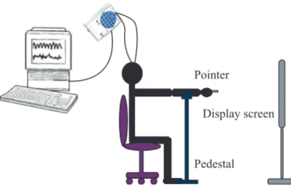
A template of a four-cycle spiral was made on a paper and placed 80 cm in front of the volunteer. It was asked to the subject to sit with the back at upright position and with the feet on the loor. The volunteer should hold a laser pen and trace the spiral templates at a self-paced velocity, with the forearm extended, at right angles to the trunk. The subjects were asked to draw two samples of a Spiral of Archimedes with their dominant hand and then stood still. The irst sample was collected with the subject drawing the spiral from its centre to its extremity (outgoing spiral - OS), whereas for the second sample the subject drew the spiral from its extremity to its centre (ingoing spiral - IS), and the third sample was collected with the subject stood still (standing still - S) pointing the laser to the center of the spiral (Miralles et al., 2006). This procedure was repeated three times for each subject and each collection time was approximately 30 seconds. EEG signal was collected while the volunteer performed the tasks. Figure 1 depicts the basic elements involved in data collection.
The acquisition of EEG signals was performed using surface electrodes. Twenty three Ag/AgCl (disks of diameter 10 mm) disk scalp electrodes, placed according to the international 10–20 system, recorded EEG, with linked earlobe reference, however, only 2 channels were used for the analysis: C3 and C4 due to the information related to motor movements they can capture. (Hema et al., 2009; Wang and Makeig, 2009). EEG was recorded with BrainNET BNT-36 (LYNX Tecnologia Eletrônica Ltda). EEG was digitized at a sampling rate of 600 Hz, with a high pass ilter of irst order at 0.1 Hz and low pass digital ilter at 100 Hz, with a 60 Hz notch ilter in each channel and a resolution of 16 bits.
The EEG spectrum is commonly divided into speciic frequency bands: 0.5-4 Hz (delta-δ), 4-8 Hz (theta-θ), 8-13 Hz (alpha-α), 13-30 Hz (beta-β), and 30-100 Hz (gamma-γ) (Nunez and Srinivasan, 2006). The predominance of a certain type of “wave”, depends on the region of the scalp that is being analyzed and the current condition of the individual. Several authors use these frequency bands in their studies, but in this study, the whole frequency range collected will be used for the calculation of the features, without the division into frequency bands, since the purpose of this study is not to characterize the aging in frequency band but the EEG signal as a whole.
The artifacts were minimized by monitoring the volunteer during the data collection, and in case of detection of any event related to movement, eye blinking, head movement, the collection was restarted. After this, an EEG expert made a careful analysis of the data to rule out potential artifact signals that the EEG could be subjected, such as muscle activity, breathing and electronic signals (Dauwels et al., 2011).
Two types of analyses were carried out. In the irst we investigated differences in the EEG signal between young (formed by groups G1 and G2) and elderly groups (formed by groups G6 and G7). In the second we considered the entire group of subjects from G1 to G7 in order to verify smoother changes that may happen over the ageing.
Features used for signal analysis
For all features described in this section, xi is the value of each sample, i represents each sample and N is the number of samples of the EEG signal.
Frequency domain features
Frequency analysis (energy estimate) was performed on the EEG signal digitized by using the Welch’s method with a 32-data point Hanning window, in order to allow analysis of the features in the frequency
domain and to calculate the features F20, F50 F80, F95 and fmean.
From the power spectrum Sx of the signal, obtained from the Fourier transform, the total power of the signal was computed using Equation 1.
1
( ) =
= ∑N
total x i
P S i (1)
Where Sx(i) is the power of the spectrum at bin i. From the power spectrum Sx and Ptotalof the signal, the following features were estimated:
Mean Frequency, which is deined in Equation 2.
( ) ( )
( )
1 1 = = ⋅ ∑ = ∑ N x i mean N x iS i f i f
S i
(2)
Where fmean is the mean frequency and f(i) is the frequency of the spectrum at bin i.
Frequency of 20%: it is the frequency for which 20% of the total power of Sx(P20) is below it.
1
20 ( ) 0.20 =
=∑N x × ∆ ≤ × total
i
P S i f P (3)
Frequency of 50%: it is also known as the median frequency. It is the frequency that divides the area under Sx into two equal parts (P50).
1
50 ( ) 0.50 =
=∑N x × ∆ ≤ × total
i
P S i f P (4)
Frequency of 80%: it is the frequency for which 80% of the total power of Sx(P80) is below it.
1
80 ( ) 0.80 =
=∑N x × ∆ ≤ × total
i
P S i f P (5)
Frequency of 95%: it is the frequency for which 95% of the total power of Sx(P95) is below it.
1
95 ( ) 0.95 =
=∑N x × ∆ ≤ × total
i
P S i f P (6)
Alpha, Beta, Delta, Theta and Gamma
The signal was iltered for each wave frequency band commonly used for the study of the EEG signal (Alpha, Beta, Delta, Theta and Gamma) for the calculation of features for these frequency bands. After iltering, we calculated the power spectrum in each band of the iltered signal (SxAlpha, SxBeta, SxDelta, SxThetaand SxGamma), obtained from the Fourier transform. From the spectrum of the signal of each band was calculated power of each band according to Equation 1, generating features:
1
( ) =
= ∑N xAlpha i
Alpha S i (7)
1
( ) =
= ∑N xBeta i
Beta S i (8)
1
( ) =
= ∑N xDelta i
Delta S i (9)
1
( ) =
= ∑N xTheta i
Theta S i (10)
1
( ) =
= ∑N xGamma i
Gamma S i (11)
Square of the Power Spectrum
The value of this feature is obtained by the quadratic sum of the power, as suggested by Hosseini and Bethge (2009). 2 1 ( ( )) N x i
E S i
=
= ∑ (12)
Signal Energy– Alpha, Signal Energy– Beta, Signal Energy– Delta, Signal Energy–Theta and Signal Energy-Gamma
These features were calculated according to Equation 12, from the spectrum of the iltered EEG signal from each band. The deinition of each feature is given below.
2 1 ( ( )) N xAlpha i
SignalEnergy Alpha S i
=
− = ∑ (13)
2 1 ( ( )) N xBeta i
SignalEnergy Beta S i
=
− = ∑ (14)
2 1 ( ( )) N xDelta i
SignalEnergy Delta S i
=
− = ∑ (15)
2 1 ( ( )) N xTheta i
SignalEnergy Theta S i
= − = ∑ (16) 2 1 ( ( )) N xGamma i
SignalEnergy Gamma S i
=
− = ∑ (17)
Time domain features
Root Mean Square (RMS) value
It is deined as the square root of the average squared instantaneous signal values and it can be calculated by using Equation 18.
2 1 1 N rms i i x x N =
= ∑ (18)
Zero Crossings (ZC)
noise-induced. Given two consecutive samples xi and
xi+1, the counting of zero crossings, ZC, is increased if:
{
1} {
1}
1
0 and 0 or 0 e 0 and
i i i i
i i
x x x x
x x
+ +
+
> < < >
− ≥ ε (19)
Variance
It is a measure of statistical dispersion, indicating the degree of variability in certain situations. It can be calculated according to Equation 20 by summing the squares of the difference between an observed value and average value.
2 1 ( ) 1 N i i x x V N = − = ∑
− (20)
Where:
x - average value of EEG signal. Standard deviation
Standard Deviation is the root square of the Variance. Its calculation is given by:
2 1 ( ) 1 N i i x x N = − σ = ∑
− (21)
Kurtosis
This is a calculation that determines the degree of latness of a distribution, investigating whether it is more tapered or lattened compared to the pattern characterized as normal. Briely, the higher the kurtosis thegreater the presence of values that are distant from average (Oja, 1981). Kurtosis is deined as:
4
4 (xi x) C=∑ −
σ (22)
Skewness
It has the purpose of verifying and calculating the data symmetry, indicating the probability of variable distribution (Oja, 1981). The value of skewness is deined as: 3 1 3 ( ) ( 1) N i i x x skew N = − ∑ =
− σ (23)
Approximate Entropy (ApEn)
Approximate Entropy is a statistical measure used to quantify the regularity and variability of a inite time signal (Ignaccolo et al., 2009; Pincus, 1991).
The entropy of the EEG measures the activity of cortical pyramidal cells, describing the irregularity, complexity or uncertainty degree of the EEG signal. The entropy of the EEG signal was calculated in time domain, as in Pincus (1991) and Shannon (1948).
Considering a sequence of signals with N samples (x(1), x(2), ..., x(N)), it is necessary to determine two
values for the calculation of the approximate entropy: the size of a pattern composed of (w) elements and the similarity criterion (µ) or tolerance (Bruhn et al., 2001; 2003; Burioka et al. 2003) for comparison of patterns. Thus, two patterns are considered similar when their difference is less than µ.
Entropy was applied to EEG signal with a value of
w (standard size) equal to 2 and a value of µ (criterion of similarity or tolerance) equal to 0.2*σ(S(x)), where σ(S(x)) is the standard deviation of S(x), as suggested by Pincus (1991).
As Sx is the set of all patterns contained in the power spectrum and Nw(σ) the number of similar patterns, it is possible to get the average of all calculated values. Thus, Nw(σ) measures the regularity or frequency of patterns similar to a given standard, allowing the approximate entropy can be deined according to Equation 24:
1
( ) ( , , ( )) ln
( ) w w
N ApEn w S x
N +
µ
µ =
µ
(24)
Linear Discriminant Analysis (LDA)
This is a method used for classiication and dimensional reduction of data, assuming that groups or classes are linearly separable and, if possible to estimate new features, designed to optimized axes that maximize the separability between classes (Kim et al., 2003).
The technique used in this study to estimate the LDA-value, was originally described by Cavalheiro et al. (2009) in a study that examines the relationship between postural control and aging, using Genetic Algorithms (GA) as a search method to solve optimization problems (Wright, 1991). It was recently used to study the correlation between human tremor and aging in Almeida et al. (2010), justifying its applicability in the context of this research between EEG and aging. The steps of the method consisted of:
• Step 1: data representation (Cn) in a space with multidimensional angular coordinates, where n
is the number of features, r is the radius and θ is the angle as shown in Equations (25), (26) and (27).
2 2 2 2
1 2 3 ... n
r= C +C +C + +C (25)
1 2 3 1
{ , , , , n−}
θ = θ θ θ θ (26)
1 2 1 3
1 2 2 2
1 1 2
1
1 2 2
1 1
tan tan , ...
tan n
n
n
C C
C C C
C
C ... C
− − − − −
θ = θ =
+
θ =
+ +
• Step 2: projection of the data in a particular axis as shown in Equation (28), resulting in a single scalar, p, or a new characteristic.
1 2
1 2
1 1
100 cos( ) cos( )
cos( n n )
LDA r
∧ ∧
∧ − −
= ⋅ ⋅ θ + θ ⋅ θ + θ ⋅
⋅ θ + θ
(28)
Where θˆ is the rotation angles which maximizes
class separability.
• Step 3: Start of GA implementation with the deinition of an initial population θˆ ,0 created from a sampling of imaginary axes, whose possible values ranged from 0 to 2π.
• Step 4: using the set of projections to calculate the accuracy estimator EZ as shown in Equation 29, where ξ is the number of classes, xi and σ2
xi are
the mean and variance of the ith class, xj and σ2
xj
are the mean and variance of the jth class.
1
2 2
1 1
( )
, 1, 2,...,
i j
i j z
i j i
x x
x x
E Z n
ξ ξ−
= = +
−
=∑ ∑ =
σ + σ (29)
• Step 5: Calculation of EZ value, which is the itness
function of GA for each imaginary axis resulting in a vector Vec, as shown in Equation 30.
1 2 z z z n E E Vec E = = = =
(30)
• Step 6: Selection by the roulette wheel technique, a sampling method with replacement commonly used in GA (Kim et al., 2003; Wright, 1991) to randomly select individuals from one generation to build the basis for the next generation. • Step 7: Generation of three descendants (θ^child1,
θ
^
child2 and θ ^
child3) according to Equations 31, 32 and 33 where only the top two offspring are selected with regard to values of their itness functions (EZ).
1 1 2
ˆ 1.5 ˆ 0.5 ˆ child parent parent
θ = θ − θ (31)
2 1 2
ˆ 0.5 0.5 ˆ ˆ child parent parent
θ = θ + θ (32)
3 1 2
ˆ 0.5ˆ 1.5 ˆ child parent parent
θ = − θ + θ (33)
• Step 8: random change of some individuals of K (Table 2), resulting in a new population (θ^current).
• Step 9: location of the imaginary axis (θ^) that maximizes the separation of classes and the relevance of the features used in the analysis. • Step 10: Repeat the process for each of the available
features. A feature is considered to be irrelevant
to the discrimination when the difference between
EZ and EZnew is less than 1% of the value of E Z.
Results and Discussion
Comparison between young and elderly groups
Initially, it was considered for data analysis groups composed of 20 young adults (group 01 and 02, age range 29.4 ± 4.93 years) and 12 elderly (group 06 and 07, age range 77.83 ± 3.97 years).
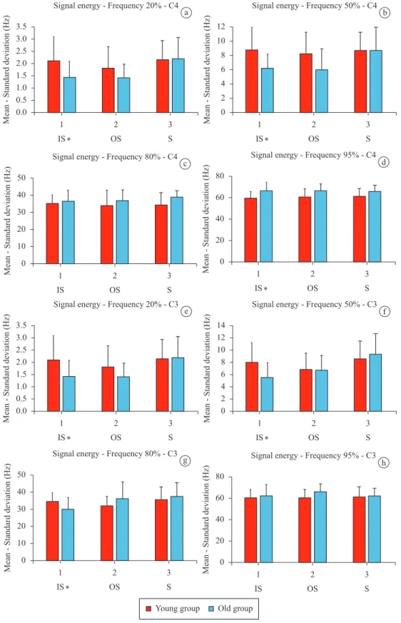
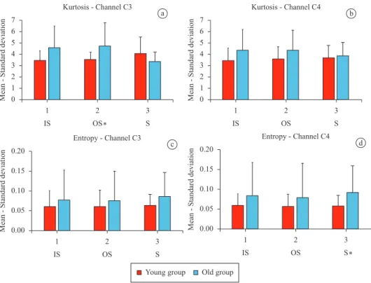
As each task was performed three times for each volunteer, the features used were extracted from the EEG signal and then it was estimated the mean of the features for each task. After doing so for each young or elderly volunteer, it was calculated the mean and standard deviation of each feature for each group (young or elderly) and plotted to look for possible signiicant differences between the groups by means of graphical analysis. Thus, possible features that would have signiicant differences between groups were selected, which are the kurtosis and Approximate Entropy of EEG signal and some features related to frequency (F20, F50, F80 and F95). On these features it was performed the normality test Shapiro-Wilk. After carrying out the normality test, the analysis of variance (ANOVA) was applied on each task and features to determine whether the observed difference is signiicant from the variations obtained. Figures 2 and 3 show graphically the mean and standard deviation obtained for the features used for the comparison of young and elderly individuals, considering the tasks IS, OS and S. Thus, even with different averages, one can verify that the differences are suficient to be considered relevant. A probability (p-value) less than 0.05 (p < 0.05) was deined as threshold of signiicance. Features that have reached signiicant differences between groups were marked with an asterisk.
Results obtained from the Linear Discrimination Analysis
After analysis of the EEG signals between adults and young people using the groups G1-G2 and G6-G7 it was possible to verify that some features extracted from EEG signals, depending on the collection task, are able to separate the groups. However, such features, when analyzed individually, showed no correlation when the study involved all age groups (G1 to G7).
a b
c d
e f
g h
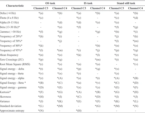
were identiied as being relevant to the calculation of the LDA-value, according to the application of step 10. The use of these features maximizes the separability between the groups. The letters in Table 1 represent those features used in Equations 34 to 42
2 2 2 2 2 2
... ...
r= a +b +c + +z +A + +M (34)
1 1
1 2 2 2
1
36 2 2
tan ; tan ;
tan
...
b c
a a b
c a L − − −
θ = θ =
+
θ =
+ +
(35)
_ 1 2
3 4 5
6 7 8
9
100 cos( 0.40) cos( 0.81) cos( 3.07) cos( 2.76) cos( 0.49) cos( 1.78) cos( 1.94) cos( 0.25) cos( 0.56) co
value IN
LDA = ⋅ ⋅r θ + ⋅ θ +
⋅ θ + ⋅ θ + ⋅ θ +
⋅ θ + ⋅ θ + ⋅ θ +
⋅ θ + ⋅ 10 11
12 13 14
15 16 17
18 19
s( 1.01) cos( 0.90) cos( 1.64) cos( 3.67) cos( 0.77) cos( 0.69) cos( 1.57) cos( 1.29) cos( 1.83) cos( 0.23)
θ + ⋅ θ +
⋅ θ + ⋅ θ + ⋅ θ +
⋅ θ + ⋅ θ + ⋅ θ +
⋅ θ + ⋅ θ + 20
21 22 23
24 25 26
27 28 29
cos( 5.11) cos( 0.59) cos( 0.45) cos( 1.13) cos( 1.74) cos( 0.82) cos( 1.35) cos( 3.68) cos( 1.91) cos( 2.
⋅ θ +
⋅ θ + ⋅ θ + ⋅ θ +
⋅ θ + ⋅ θ + ⋅ θ +
⋅ θ + ⋅ θ + ⋅ θ +
30 31 32
33 34 35
36
01) cos( 1.73) cos( 1.10) cos( 0.73) cos( 1.31) cos( 0.31) cos( 0.75) cos( 0.63)
⋅ θ + ⋅ θ + ⋅ θ +
⋅ θ + ⋅ θ + ⋅ θ +
⋅ θ +
(36)
2 2 2 2 2 2
... ...
r= a +b +c + +z +A + +H
(37)
1 1
1 2 2 2
1
38 2 2
tan ; tan ;
tan
...
b c
a a b
c a G − − −
θ = θ =
+
θ =
+ +
(38)
_ 1 2
3 4 5
6 7 8
9
100 cos( 2.97) cos( 2.90) cos( 2.54) cos( 6.69) cos( 2.33) cos( 0.64) cos( 2.89) cos( 2.31) cos( 0
value OUT
LDA = ⋅ ⋅r θ + ⋅ θ +
⋅ θ + ⋅ θ + ⋅ θ +
⋅ θ + ⋅ θ + ⋅ θ +
⋅ θ + 10 11
12 13 14
15 16 17
18
.28) cos( 0.64) cos( 2.45) c os( 0.89) cos( 2.80) cos( 2.81) cos( 2.60) cos( 2.44) cos( 2.94) c os( 1.03)
⋅ θ + ⋅ θ +
⋅ θ + ⋅ θ + ⋅ θ +
⋅ θ + ⋅ θ + ⋅ θ +
⋅ θ + ⋅ 19 20
21 22 23
24 25 26
27
cos( 1.34) cos( 2.00) cos( 1.30) cos( 1.92) cos( 1.82) c os( 0.87) cos( 2.29) cos( 1.39) cos( 0.21) cos(
θ + ⋅ θ +
⋅ θ + ⋅ θ + ⋅ θ +
⋅ θ + ⋅ θ + ⋅ θ +
⋅ θ + ⋅ θ28 29
30 31 32
33 34 35
36 37
2.11) cos( 0.24) c os( 2.30) cos( 2.34) cos( 0.55) cos( 1.28) cos( 0.17) cos( 2.79) c os( 0.06) cos( 1.
+ ⋅ θ +
⋅ θ + ⋅ θ + ⋅ θ +
⋅ θ + ⋅ θ + ⋅ θ +
⋅ θ + ⋅ θ + 39) cos(⋅ θ +38 2.36) (39)
2 2 2 ... 2 2 ... 2
r= a +b +c + +z +A + +N (40)
1 1
1 2 2 2
1
38 2 2
tan ; tan ;
tan
...
b c
a a b
c a M − − −
θ = θ =
+
θ =
+ + (41) a c b d
Figure 3. Mean values obtained for features, tasks OS, IS and S. Error bars represent the standard deviation. The asterisk indicates signiicant
_ 1 2
3 4 5
6 7 8
9 10
100 cos( 5.49) cos( 2.02) cos( 0.32) cos( 6.41) cos( 5.52) cos( 2.64) cos( 0.03) cos( 3.48) cos( 2.39) cos( 2
value S
LDA = ⋅ ⋅r θ + ⋅ θ +
⋅ θ + ⋅ θ + ⋅ θ +
⋅ θ + ⋅ θ + ⋅ θ +
⋅ θ + ⋅ θ + 11
12 13 14
15 16 17
18 19 20
.55) cos( 0.36) c os( 2.51) cos( 2.47) cos( 1.27) cos( 1.34) cos( 2.03) cos( 2.42) c os( 2.23) cos( 17.24) cos( 2.2
⋅ θ +
⋅ θ + ⋅ θ + ⋅ θ +
⋅ θ + ⋅ θ + ⋅ θ +
⋅ θ + ⋅ θ + ⋅ θ +
21 22 23
24 25 26
27 28 29
9) cos( 2.38) cos( 2.48) cos( 2.70) c os( 0.84) cos( 1.11) cos( 2.17) c os( 1.19) cos( 2.84) cos( 2.13)
⋅ θ + ⋅ θ + ⋅ θ +
⋅ θ + ⋅ θ + ⋅ θ +
⋅ θ + ⋅ θ + ⋅ θ +
30 31 32
33 34 35
36 37 38
c os( 0.78) cos( 3.22) cos( 10.47) cos( 1.78) cos( 0.78) cos( 0.80) c os( 1.23) cos( 3.12) cos( 8.04)
⋅ θ + ⋅ θ + ⋅ θ +
⋅ θ + ⋅ θ + ⋅ θ +
⋅ θ + ⋅ θ + ⋅ θ +
(42)
Description of parameters used to calculate the LDA-value
In this study the dimension of the feature vector is that given in Table 2. Each of its elements corresponds to the 22 calculated features. Those features that have an insigniicant impact on the inal discrimination of the groups were excluded, following the criteria of the LDA.
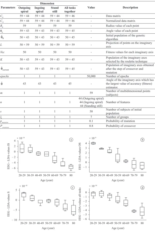
For discussion and analysis of results, it was used the Boxplot. Figure 4 show the LDA-values obtained
for the seven groups in this study. A visual analysis of the boxplot graph shows that the LDA-value is a feature that has its value changed with age. When estimating the correlation between the LDA-value and age, it was obtained a Pearson correlation coeficient between 0.83 to 0.89 for different tasks (IS, OS and S), indicating a high degree of correlation between these variables.
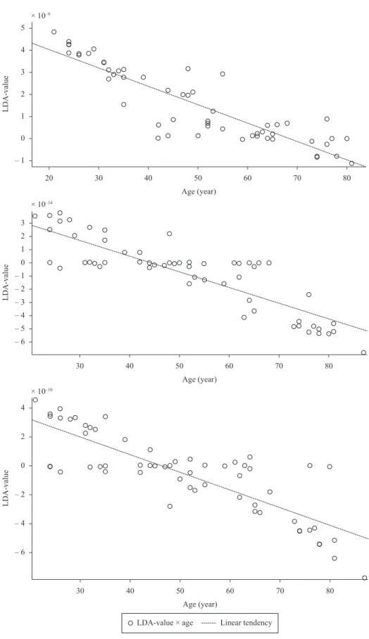
Comparing and analyzing the boxplots in Figure 4, it is observed that the median lines will decrease in function of age. The analysis of Figure 4(c) suggest that the groups G6 (70 to 79 years) and G7 (80 years) have the highest whiskers that is, there are no outliers. In the same groups, a larger distance between the median lines and the third quartile is also highlighted which lead to think, although with no statistical difference, that the data from G7 group tend to be larger than those from G6 group and that they have a higher dispersion. This happens because the interquartile size as well as the whiskers are larger. The LDA-values are shown in Figure 5 in all the tasks performed by the subjects (IS, OS and S) . It is clearly visible the linear trend of the LDA-values with increasing age.
Table 1. Relevant features to calculate the LDA-value.
Characteristic OS task IS task Stand still task
Channel C3 Channel C4 Channel C3 Channel C4 Channel C3 Channel C4
Delta (<4 Hz) *(a) *(b) *(a) *(b) *(a) *(b)
Theta (4 a 8 Hz) *(c) - *(c) - *(c) *(d)
Alpha (8-13 Hz) - *(d) *(d) *(e) *(e)
-Beta (13-30 Hz)* - *(e) *(f) - *(f) *(g)
Gamma ( >30 Hz) *(f) *(g) - *(g) *(h) *(i)
Frequency of 20%* *(h) *(i) - - *(j) *(k)
Frequency of 50%* - *(j) - - *(l) *(m)
Frequency of 80%* *(k) - - *(h) *(n) *(o)
Frequency of 95%* *(l) *(m) *(i) *(j) *(p) *(q)
Mean frequency *(n) *(o) *(k) *(l) *(r) *(s)
Zero Crossings (ZC) *(p) *(q) - *(m) *(t) *(u)
Root Mean Square (RMS) *(r) *(s) *(n) *(o) - *(v)
Signal energy – delta *(t) *(u) *(p) *(q) *(x)
-Signal energy - theta *(v) *(x) *(r) - *(z)
-Signal energy - alpha *(z) *(A) *(s) *(t) *(A) *(B)
Signal Energy - Beta * *(B) *(C) *(u) *(v) *(C) *(D)
Signal energy - gamma *(D) *(E) *(x) *(z) *(E) *(F)
Kurtosis* *(F) *(G) *(A) *(B) *(G) *(H)
Skewness *(H) *(I) *(C) *(D) *(I) *(J)
Variance *(J) *(K) *(E) *(F) *(K) *(L)
Standard deviation *(L) *(M) - *(G) *(M) *(N)
Approximate entropy *(N) - *(H) - -
Table 2. Parameters used to calculate the LDA-value.
Parameters
Dimension
Value Description
Outgoing spiral
Ingoing spiral
Stand still
All tasks together
C0 59 × 44 59 × 44 59 × 44 59 × 46 - Data matrix
CN 59 × 44 59 × 44 59 × 44 59 × 46 - Normalized data matrix
R0 59 59 59 59 - Radius value of each point
θ0 59 × 43 59 × 43 59 × 43 59 × 45 - Angle value of each point
0
ˆ
θ 50 × 43 50 × 43 50 × 43 50 × 45 - Initial population of the genetic algorithm
L 50 × 59 50 × 59 50 × 59 50 × 59 - Projection of points on the imaginary axis
Vec 50 50 50 50 - Fitness values for each imaginary axis
K 50 × 43 59 × 43 59 × 43 59 × 45 - Population of the imaginary axes selected by the roulette technique
ˆ current
θ 50 × 43 59 × 43 59 × 43 59 × 45
-Population of imaginary axes obtained after the step of crossover and mutation
epochs 1 1 1 1 50,000 Number of epochs
ˆ
θ 43 43 43 45
-Angle of the imaginary axis which has the largest value of accuracy (itness) estimator.
m 1 1 1 1 59 Number of multidimensional points
(subjects)
n 1 1 1 1
44 (Outgoing spiral) 44 (Ingoing spiral)
44 (Standing still)
Number of features
s 1 1 1 1 50 Number of subjects of initial
population
ξ 1 1 1 1 7 Number of groups
pmutation 1 1 1 1 0.1 Probability of mutation
Pcrossover 1 1 1 1 0.8 Probability of crossover
a b
c d
Figure 4. Boxplot of LDA-values, 07 groups of volunteers. a) Ingoing spiral task - IS. Pearson correlation coeficient obtained: 0.85.
Conclusion
In this study it was veriied the correlation between EEG signal and age. The features of the EEG signal were able to separate groups of volunteers between different age ranges (20-80 years). In the irst analysis signiicant differences between young and old groups were veriied. In the second analysis, LDA was introduced as a new method for investigation of EEG signals.
Statistical analysis was aimed to generate results consistent with the formulated hypothesis: “It is possible to correlate the EEG signals with aging, indicating the separability between groups of distinct subjects in different age ranges.”
For this study the EEG signals from electrodes C3 and C4 were analyzed. Initially signiicant differences were observed between groups of young and elderly. In this irst analysis, few features could distinguish these groups. However, the features that have achieved the differentiation were not the same for electrodes C3 and C4. In relation to the electrode C4, the features that made the difference were F20, F50, F95 and
Approximate Entropy, for the electrode C3 these were
F20, F50, F80 and kurtosis. The two electrodes were able to capture signiicant differences in measures of frequency of the EEG signal, however, only the electrode C4 managed a noteworthy distinction between the groups due to the increased complexity of the EEG signal with age (Approximate Entropy feature).
According to Nitish and Tong (2004) and Thompson et al. (2008), EEG signals of individuals over 80 years old may present reduction in frequency and amplitude and propensity to gradually slowing of alpha rhythm corresponding to a rate of mental deterioration. However, regardless of age, healthy elderly people have strokes of EEG signals which are visually dificult to distinguish from those of a young individual. In this sense, the results of this research show the LDA-value as a relevant feature for the analysis and separability of EEG signals between different age ranges, with potential applicability in other studies related to the area.
Ehlers and Kupfer (1989), also afirm the dificulty of differentiating the EEG signals according to age and add that it can occur minor changes in the EEG signals for the elderly. Through the LDA this study demonstrated satisfactorily, through the quantitative analysis of EEG signals, the separability of a group of healthy subjects in different age ranges.
In this context, this research irstly presents in quantitative manner, the ability to distinguish or separate these traces by means of the methodology used. Probably this was possible as a result of the
joint analysis of several features, leading to the hypothesis that only the study of a feature linked to a physiological phenomenon is not able to quantify changes with age, but the combined analysis of various physiological phenomena can quantify and discriminate the changes over aging. This conclusion shows the validity of the LDA as an analysis tool, as well as the need to use other statistical methods to expand the possibilities of observing the results obtained in each stage of the research.
Cavalheiro et al. (2009), obtained satisfactory results in the study and analysis of postural control, measured by the displacement of the Center of Pressure(COP), in groups of young and elderly adults through the LDA. The technique used, the LDA, was differently introduced in this work as a method for analysis of EEG signals. The results also indicated that the LDA-value was effective in the separability between groups, exhibiting a high degree of correlation (0.85, 0.89, 0.83 and 0.87) with age.
Most studies in the literature are related to the analysis of EEG signals associated with some pathology (Bennys et al., 2001; Bonanni et al., 2008; Dauwels et al., 2011; Faust et al., 2007; Natarajan et al., 2004) which demonstrates the lack of studies with the purpose of understanding the complex relationship between the EEG signal of healthy subjects and the aging. This study included only healthy subjects.
The conclusions drawn from the results obtained using the LDA show that it is possible to develop further researches on the changes brought about by the age in the human body, assisting specialists in the search for new tools and solutions that promote the improvement of life quality.
Currently, EEG has established use as an auxiliary method in the diagnosis of diseases, especially when the diagnosis remains open. Analyses and studies in this research may enable the establishment of EEG patterns of healthy subjects allowing clinical management options by comparing the CNS related pathologies and considered normal EEG patterns in different groups and ages.
It is expected that the methods presented in this research, further contribute to early detection of diseases related to the CNS, aiding in its diagnosis, quantifying the severity of each case, or to monitor their progress in establishing a safer prediction of the disease, seeking ensure appropriate clinical care and facilitate the planning of resources needed.
Acknowledgements
References
Almeida MFS, Cavalheiro G, Pereira AA, Andrade AO. Investigation of age-related changes in physiological kinetic tremor. Annals of Biomedical Engineering. 2010; 38:3423-39. PMid:20571851. http://dx.doi.org/10.1007/s10439-010-0098-z
Anokhin AP, Birbaumer N, Lutzenberger W, Nikolaev A, Vogel F. Age increases brain complexity. Electroencephalography and clinical Neurophysiology. 1996; 99:63-8. http://dx.doi. org/10.1016/0921-884X(96)95573-3
Bennys K, Rondouin G, Vergnes C, Touchon J. Diagnostic value of quantitative EEG in Alzheimer’s disease. Clinical Neurophysiology. 2001; 31:153-60. http://dx.doi.org/10.1016/ S0987-7053(01)00254-4
Bonanni L, Thomas A, Tiraboschi P, Perfetti B, Varanese S, Onofrj M. EEG comparisons in early Alzheimer’s disease, dementia with Lewy bodies and Parkinson’s disease with dementia patients with a 2-year follow-up. Brain: A Journal of Neurology. 2008; 131:690-705. PMid:18202105. http:// dx.doi.org/10.1093/brain/awm322
Bruhn JL, Lehmann E, Ropcke H, Bouillon TW, Hoeft A. Shannon entropy applied to the measurement of the electroencephalographic effects of desflurane. Anesthesiology. 2001; 95:30-5. PMid:11465580. http:// dx.doi.org/10.1097/00000542-200107000-00010 Bruhn JT, Bouillon W, Radulescu L, Hoeft A, Bertaccini E, Shafer SL. Correlation of approximate entropy, bispectral index, and Spectral Edge Frequency 95 (SEF95) with clinical signs of “Anesthetic Depth” during coadministration of propofol and remifentanil. Anesthesiology. 2003; 98:621-7. PMid:12606904. http://dx.doi.org/10.1097/00000542-200303000-00008
Burioka N, Cornélissen G, Halberg F, Kaplan DT, Suyama H, Sako T, Shimizu E. Approximate entropy of human respiratory, movement during eye-closed waking and different sleep. American College of Chest Physicians. 2003;123:80-6. PMid:12527606. http://dx.doi.org/10.1378/chest.123.1.80 Cavalheiro G, Almeida MFS, Pereira AA, Andrade AO. Study of age-related changes in postural control during quiet standing through Linear Discriminant Analysis. BioMedical Engineering OnLine. 2009; 8:35. PMid:19922638. PMCid:2785821. http://dx.doi.org/10.1186/1475-925X-8-35 Dauwels J, Srinivasan K, Reddy MR, Musha T, Vialatte FB, Latchoumane C, Jeong J, Cichocki A. Slowing and loss of complexity in Alzheimer’s EEG: Two sides of the same coin? International Journal of Alzheimer’s Disease. 2011; 2011: 539621. http://dx.doi.org/10.4061/2011/539621 Ehlers CL, Kupfer DJ. Effects of age on delta and REM sleep parameters. Electroencephalography and Clinical Neurophysiology. 1989; 72:118-25. http://dx.doi. org/10.1016/0013-4694(89)90172-7
Evans RJ, Abarbanel A. Introduction to Quantitative EEG and neurofeedback. San Diego: Academic Press; 1999. Faust O, Acharya RU, Allen AR, Lin CM. Analysis of EEG signals during epileptic and alcoholic states using
AR modeling techniques. IRBM. 2007; 29(1):44-52. http:// dx.doi.org/10.1016/j.rbmret.2007.11.003
Ferri CP, Prince M, Brayne C, Brodaty H, Fratiglioni L, Ganguli M, Hall K, Hasegawa K, Hendrie H, Huang Y, Jorm A, Mathers C, Menezes PR, Rimmer E, Scazufca M, Alzheimer’s Disease International. Global Prevalence of Dementia: a Delphi Consense study. The Lancet. 2005; 366(9503):2112-17. http://dx.doi.org/10.1016/ S0140-6736(05)67889-0
Frankel JE, Bean JF, Frontera WR. Exercise in the elderly: Research and clinical practice. Clinics in Geriatric Medicine. 2006; 22:239-56. PMid:16627076. http://dx.doi.org/10.1016/j. cger.2005.12.002
Hema CR, Paulraj MP, Yaacob S, Adom AH, Nagarajan R. EEG motor imagery classiication of hand movements for a Brain Machine Interface. Biomedical Soft Computing and Human Sciences, 2009; 14:49-56.
Hosseini R, Bethge M. Spectral stacking: Unbiased shear estimation for weak gravitational lensing [Internet]. Max Planck Institute for Biological Cybernetics, 2009. Available from: http://www.kyb.mpg.de/ileadmin/user_upload/iles/ publications/attachments/MPIK-TR-186_6114%5b0%5d.pdf. Ignaccolo M, Latka M, Jernajczyk W, Grigolini P, West BJ. The dynamics of EEG entropy. Journal of biological physics. 2009; 36:185-96. PMid:19669909. PMCid:2825306. http:// dx.doi.org/10.1007/s10867-009-9171-y
Kim HC, Kim D, Bang SY. Extensions of LDA by PCA mixture model and class-wise features. Pattern Recognition. 2003; 36:1095-105. http://dx.doi.org/10.1016/S0031-3203(02)00163-2
Miralles F, Tarongi S, Espino A. Quantiication of the drawing of an Archimedes spiral through the analysis of its digitized picture. Journal of Neuroscience Methods. 2006;152:18-31. PMid:16185769. http://dx.doi. org/10.1016/j.jneumeth.2005.08.007
Natarajan K, Acharya UR, Alias F, Tiboleng T, Puthusserypady SK. Nonlinear analysis of EEG signals at different mental states. BioMedical Engineering OnLine. 2004; 3:7. PMid:15023233. PMCid:400247. http://dx.doi.org/10.1186/1475-925X-3-7
Nitish VT, Tong S. Advances in Quantitative Electroencephalogram analysis methods. Annual Review of Biomedical Engineering. 2004; 6:453-95. PMid:15255777. http://dx.doi.org/10.1146/annurev.bioeng.5.040202.121601 Nunez PL, Srinivasan R. Electric ields of the brain. 2nd ed. New York: Oxford University Press; 2006. http://dx.doi. org/10.1093/acprof:oso/9780195050387.001.0001 Oja H. On location, scale, skewness and kurtosis of univariate distributions. Scandinavian Journal of Statistics. 1981; 8:154-68.
Pincus SM. Approximate entropy as a measure of system complexity. Proceedings of the National Academy of Science. 1991; 88:2297-301. http://dx.doi.org/10.1073/ pnas.88.6.2297
Thompson T, Steffert T, Ros T, Leach J, Gruzelier J. EEG applications for sport and performance. Methods. 2008; 45:279-88. PMid:18682293. http://dx.doi. org/10.1016/j.ymeth.2008.07.006
Tucker AM, Dinges DF, Hans PA, Dongen V. Trait interindividual differences in the sleep physiology of healthy young adults. Journal of Sleep Research. 2007; 16:170-80. P M i d : 1 7 5 4 2 9 4 7 . h t t p : / / d x . d o i . o rg / 1 0 . 1111 / j.1365-2869.2007.00594.x
Wang Y, Makeig S. Predicting intended movement direction using EEG from human posterior parietal cortex. Lecture Notes in Computer Science. 2009; 5638/2009:437-446. http://dx.doi.org/10.1007/978-3-642-02812-0_52 Wright AH. Genetic algorithms for real parameter optimization. In: Rawlins GJE. Foundations of genetic algorithms. San Mateo: Morgan Kaufmann; 1991. p. 205-18.
Autores
Lilian Ribeiro Mendes de Paiva, Adriano Alves Pereira*, Maria Fernanda Soares de Almeida, Guilherme Lopes Cavalheiro, Selma Terezinha Milagre, Adriano de Oliveira Andrade