Development of a Fully Coupled Approach for Evaluation of Wellbore Stability in Hydrocarbon Reservoirs

(1)

ISSN 1553-345X

Development of a Fully Coupled Approach for Evaluation of Wellbore Stability in Hydrocarbon Reservoirs

Vera Rocca

DITAG Department, Politecnico di Torino, Corso Duca degli Abruzzi 24, 10129 Torino, Italy

Abstract: Problem statement: When a well is drilled in a hydrocarbon reservoir, the original thermodynamic conditions are altered, the natural stresses are redistributed and a stress concentration occurs around the hole. The alteration of the original equilibrium can lead to wellbore damage, sometimes to its complete collapse. Loss of time associated with stability problems is estimated to account for 12-15% of drilling costs world-wide. Approach: The adoption of a reliable modeling approach to predict instability due to time-dependent alteration of natural equilibrium is fundamental for the optimization of drilling plans, completion design and production activities. Results: In this study the possibility of investigating instability phenomena in terms of both stress-strain and thermo-dynamic formation behavior through a fully coupled thermo-porous-elastic-plastic approach is demonstrated. According to the fully coupled approach, porous flow, temperature development and stress-strain calculations are performed together: the whole system is discretised on one grid domain and solved simultaneously for both the thermodynamic and the geomechanical variables. For the plastic analysis implementation, an iteratively coupled approach was adopted inside the fully coupled routine: the model basic equations (porous flow and rock deformation) and the plastic behavior equations were solved separately and sequentially at each non-linear iteration. The iterative coupling approach corresponds to an implicit treatment of the plastic variables, essential to preserve the stability of the elasto-plastic solution. The key points of the model analytical formulation, of the numerical formalization as well as of the implementation of the adopted solutions to make the thermo-porous-elastic-plastic model applicable to assess wellbore stability are presented. Conclusion: The proposed model was first validated and then applied to several synthetic and real cases. In this study the effectiveness of the developed model to investigate the potential impact of instability phenomena on the well drilling design is demonstrated also by discussing the results from a case history.

Key words: Implicit coupling approach, iteratively coupled approach, wellbore design, Desai plastic model

INTRODUCTION

Wellbore stability related problems are reported to cost the petroleum industry more than 500 million US dollars each year[13]. In fact, alterations of natural equilibrium caused by drilling operations and extraction activities can lead to time-dependent wellbore instability phenomena, such as wall swelling and formation breakdown. Borehole instability also represents the main cause for loss of drilling fluids and consequent potential kick problems and can be so severe to compel the wellbore abandonment. In addition, sand production often associated with high production rate in poorly consolidated reservoirs can compromise oil production, increase completion costs and reduce the life of equipment.

Wellbore collapse and sand production are believed to be caused by large in-situ stresses and are the result of rock formation damage near a well. It is

highly desirable to understand the main mechanisms for rock collapse and sand production and quantify these processes in order to optimize the drilling plan phase (i.e., mud characterization, drilling trajectory, rate of penetration) the design completion phase (casing placement and cementing operations) and the production activities.

(2)

mechanics, dealing with crack propagation and geometry. Usually, each of these disciplines makes simplifying assumptions about the part of the problem that is not of its own primary interest. However, such an approach is unacceptable in situations where there is a strong coupling, such as weak plastic reservoir rocks and unconsolidated porous media[2,11]. A coupled approach, combining constitutive equations with thermal and hydraulic laws, is then required to perform accurate time-dependent analyses of stress, pore pressure and temperature variation.

The technical literature shows several theoretic approaches to model the formation behavior with different degrees of coupling between rock deformation and fluid flow: from partially coupled to fully coupled methods. Although the couplings physically exist to some extent in all systems, the need for using more complex, fully coupled geomechanical modeling is generally acknowledged to be limited to the cases of compacting reservoirs or high-pressure injection operations or severe wellbore stability problem. Starting from Charlez’s analytical thermo-porous-mechanical model formulation[1], the author of this study introduces the possibility of investigating the wellbore instability phenomena in terms of both the stress-strain and the thermo-dynamic formation behavior through a fully coupled approach. An iteratively coupled routine was adopted in the fully coupled approach in order to implement the plastic deformation analysis. The key points of both the numerical formulation and the implementation solutions developed by the author to make the thermo-poro-elasto-plastic model applicable to assess wellbore stability are presented.

MATERIALS AND MATHODS

Different degrees of coupling: A multiphysical approach, able to simulate the correlations existing between rock geomechanics and reservoir fluid dynamics, requires the characterization of both the fluid and solid system components: A fluid-flow model describing the motion of the pore fluid and a stress-deformation model reproducing the stress-deformation of the rock solid skeleton. Mass and force conservation laws and constitutive relations, which represent the coupling effects between components, are used to obtain the fluid-flow and stress-deformation model. The non-linear behaviour typical of reservoir rocks can require the adoption of specific constitutive models, such as elastic-plastic law, visco-plastic law.

The methodologies of coupling flow through porous media and solid deformation that are found in

the technical literature can be generally classified into fully coupled and partially coupled approaches.

In spite of recent advances in numerical calculation, the interaction between reservoir fluid flow and solid deformation still present a number of problems, such as accuracy, convergence issues and computing efficiency[12].

The different coupling techniques are briefly presented in the following, highlighting the main advantages and shortcomings of each methodology[3].

Fully coupled approach: In the fully coupled

approach, porous flow and displacement calculations are performed together and the software solver must handle both the thermodynamic variables, i.e., temperature and pressure and the geomechanical response, such as displacement. The method is also called implicit coupling since the whole system is discretized in one grid domain and solved simultaneously. This approach has the advantage of internal consistency. The full coupling is also the most stable technique and preserves second order convergence of nonlinear iterations. However, the adoption of this methodology may complicate the coupling of existing flow simulators with geomechanical ones; it also requires more code development than other techniques and it can be slower than the explicit and iterative methods in some situations.

Iteratively coupled approach: In the iteratively coupled approach, the basic equations for multiphase porous flow and rock deformation are solved separately and sequentially and the coupling terms are iterated at each time step. The exchange of information between the reservoir simulator and the geomechanic module is generally performed through a coupling code that also verifies the convergence of the coupling iterations. The adopted convergence criterion is typically based on pressure or stress changes between the last two solution iterations[12].

The adopted coupling variables are usually related to the key reservoir characteristics in order to highlight the most important coupling phenomena, such as volume changes, stress-dependent permeability, saturation-dependent rock strength.

(3)

Explicitly coupled approach: The explicit coupling is a special case of the iteratively coupled method: a simulator performs computations for multiphase porous flow at each time step and updates the geomechanical parameters during specified time steps, which are selected on the basis of pore volume change magnitude. If the pore volumes vary slowly during the time steps, then few geomechanical updates are required.

The main attraction of the explicitly coupled approach is the potential decrease of computational time, which is often mostly spent in calculating displacement for fluid flow/geomechanical problems. On the other hand, the explicit nature of the coupling can impose time step restriction on simulation runs in order to preserve stability and accuracy.

Model development for wellbore stability: The presented wellbore stability model was developed on the basis of the analytical approach formulated by Charlez[1] and adapted to wellbore stability issues by Sartori1[10]. It is based on a fully coupled thermo-porous-elastic-plastic philosophy, which combines the constitutive equations with the thermal and hydraulic laws.

The proposed theoretical formulation is developed for a vertical borehole in a homogeneous, isotropic, elastoplastic, saturated porous medium subject to mono-dimensional, axisymmetric stress conditions in plane state of strain. According to Charlez[1], the governing model equations can be divided into a basic group describing flow in the porous medium and rock deformation and a complementary group describing the plastic behavior of the formation.

Principal basic equations: The basic equation group consists of: conservative laws (i.e.: Equilibrium, fluid mass and entropy), diffusion laws (i.e.: Darcy’s law and Fourier’s law), strain-displacement correlation law, stress-strain constitutive law and linearized behavior laws for pressure and temperature.

The constitutive law was developed in accordance to the hypothesis that small perturbations occurred, which implied that the total deformation is equal to the sum of an elastic increment and a plastic one:

(

)

(

)

kk

0 p

ij C0 p p0 ij BK (TB T )0 ij

σ − σ = ε − ε − α − δ − α − δ (1)

Where:

σ = The stress tensor

ε = The total strain tensor

εp

= The plastic strain KB = The bulk modulus

α = The Biot’s coefficient P = The fluid pressure p0 = The reference pressure

αB = The drained thermal expansion coefficient of saturated rock

T = The temperature

T0 = The reference temperature

δij = The Kronecker tensor and C0 reads:

(

p

)

B

(

p

)

(

p

)

0 B kk kk ij B ij jj

2G

C K 2G

3

⎛ ⎞

ε − ε =_⎜ − _⎟ ε − ε δ + ε − ε

⎝ ⎠ (2)

where, GB is the bulk shear modulus. Sartori proposed a peculiar formulation for the hydraulic diffusion equation and for the thermal diffusion equation which, compared to the analogous formulations of the thermo-porous-elastic-plastic theory, contain an additional term typical of the plastic model. Combining Darcy’s law with the mass conservation principle and the hydraulic diffusion equation[1], the linearized pressure behaviour law was derived:

(

p

)

_p

0

0 0

1 p L T m 1

t T t t t t

∂ ε − ε

∂ ₋ ρ ∂ _{+ αΙ} _{+ βΙ}∂ε ₌∂

η ∂ η ∂ ∂ ∂ ∂ ρ (3)

Where:

η = The Biot modulus L = The latent heat

ρ0 = The fluid density

β = Plastic coefficient (analogous to Biot coefficient α) m = The fluid mass per unit volume

I = The identity matrix

Analogously, combining the Fourier’s law with the heat conservation principle and with the thermal diffusion equation[1], the linearized temperature behavior law was derived:

(

)

0

kk

2 2 0

0

0 0 0

p

0

B B m

L

L p 1 T

C m

T t T T t

S m

K s

t t t

ε

⎛ ρ ⎞

ρ ∂ ∂

− + ⎜_⎜ + ⎟_⎟ +

η ∂ _⎝ η ∂_⎠

∂ ε − ε ⎛∂ ∂ ⎞

α Ι =_⎜ + _⎟

∂ ⎝∂ ∂ ⎠

(4)

Where:

Cε = The heat capacity at constant volumetric

deformation

m0 = The saturated rock density S = The entropy

0 m

(4)

Complementary equations: The complementary equations, which describe the plastic behavior of the formation, were taken as in the Desai’s approach. Desai and coworkers[3-7] introduced a hierarchical approach for the development of constitutive models to account for various factors that influence the geological material behavior. This approach allows for progressive development of models of higher grades, corresponding to different levels of complexities. The basic model, termed the “δ0 model”, involves initially isotropic material, hardening isotropically with associative plasticity. In the proposed analytic formulation, the δ0 model is used to describe the rock plastic deformation because, compared with models of higher grades, it provides a particularly accurate description of shale behavior and requires a smaller number of plastic input parameters. Belonging to classic incremental plasticity, Desai’s model is based on the concepts of the yield function, f, on the plastic potential function, g and on the hardening function, αd, which are specific for the adopted plastic approach.

Desai proposed the following formulation for the yield function based on a polynomial expansion in terms of the direct invariants of the stress tensor (J1, J2, J3):

(

)

₂ ₁e n ₁e 2

(

)

m

e 2 d d d r

a a a

J ' J J

f ' , 1 S

p p p

⎛ _⎛ _⎞ _⎛ _⎞ ⎞

⎜ ⎟

σ χ = − −α −_⎜ _⎟ + γ −_⎜ _⎟ − β

⎜ _⎝ _⎠ _⎝ _⎠ ⎟

⎝ ⎠

(5)

Where:

σ’

e = The Biot’s effective stress

χ = The dimensionless trajectory of plastic strain

pa = The atmospheric pressure

αd = The dimensionless hardening function Je1 = First invariant of the elastic stress

n = The dimensionless shape change parameter

γd, βd, m = Dimensionless material response constants associated with the ultimate envelopes (i.e., the locus of points corresponding to asymptotic stress to stress-strain curves for different tests[7])

Sr = Expressed by the following equation:

( )

3

r 1.5

2 27 J ' S

2 J '

= − (6)

As the δ0 model is based on associative plasticity, the plastic potential function g is the same as the yield function.

The adopted expression for the dimensionless hardening function reads:

D

d 1 1

2 2 D

a exp 1

a

⎡ ⎛ χ ⎞⎤

α = ⎢−η χ −⎜ _{+ η χ} ⎟⎥

⎢ ⎝ ⎠⎥

⎣ ⎦ (7)

Where:

a1, η1, a2, η2 = Dimensionless hardening constants

χ = The dimensionless trajectory of plastic strain defined as follows:

p p 1/ 2 ij ij (d d )

χ =

_∫

ε ε (8)

and χD is the deviatoric part of χ.

Solution implementation: Workflow: According to the solution workflow developed by the author, the physical phenomena induced by drilling operations and/or production activities into rock formations were simulated through two computational phases: the initialization and the working phase (Fig. 1).

During initialization, the plastic properties corresponding to the undisturbed formation were derived from complementary equations. The formation is assumed to be a homogeneous medium, subject to known and uniform temperature, pore pressure and stress distribution. As the complementary equation presents no spatial derivatives and so the system is spatially decoupled and thanks to the assumption of uniform thermodynamic and geomechanic original conditions, the initial phase is solved as a zero-dimensional model. Absolute values of the initial stress tensor could be quite important, thus a gradual stress imposition approach could help minimizing convergence problems. Starting with a reference temperature and setting pore pressure and stress equal to zero, the known initial thermodynamic equilibrium and stress-strain field are reached incrementally and the corresponding plastic parameter values are calculated for each incremental step. This was achieved by solving iteratively the nonlinear complementary equation system.

(5)

INPUT

Δp=Δpi,n_,_Δ_T=_Δ_Ti,n_,_Δ_u=_Δ_ui,n_{, p=p}n-1₊_Δ_pi,n

Initialization

Δεp 0_=0,_Δλ0_=0,_Δσ0₌_Δσn,i-1_,_Δχ0₌_Δχn,i-1

OUTPUT

εp

Strain Δε computation from displacementΔu

Predictor stress computation

Elastic stress Δσe_{form stress-strain relation}

f(σe_{, p,}_χ_)?

Δλ=0

Δεp₌₀

Δχ=0

Δσ=Δσe

ELASTIC STATE

Corrector stress computation

PLASTIC STATE

Complementary equations solution through Newton-Raphson method

INPUT

Initialization

OUTPUT

εp

Strain Δε computation from displacementΔu Strain Δε computation from displacementΔu

f(σe_{, p,}_χ_)?

Δλ=0

Δεp₌₀

Δχ=0

Δσ=Δσe

ELASTIC STATE

Δλ=0

Δεp₌₀

Δχ=0

Δσ=Δσe

ELASTIC STATE

PLASTIC STATE

Complementary equations solution through Newton-Raphson method Complementary equations solution

through Newton-Raphson method

PHASE 1: INITIALIZATION

PHASE 2: WORKING PHASE

n=0

Boundary conditions

Iter i =0

Basic equations solution (u, p, T)

Complementary equations solution (εp₎

i→ i+ 1 F n → n+1 T STOP s=0

Iter j=0

Convergence? j→j+1

s → s+ 1 Convergence? F T

Incremental values imposition (ΔT, Δσ, Δp ) Initial conditions

(Tr, σ=0,p=0 )

n=0

Iter i =0

i→ i+ 1 F n → n+1 T STOP s=0

Iter j=0

(Tr, σ=0,p=0 )

INPUT

Initialization

OUTPUT

εp

Strain Δε computation from displacementΔu

f(σe_{, p,}_χ_)?

Δλ=0

Δεp₌₀

Δχ=0

Δσ=Δσe

ELASTIC STATE

PLASTIC STATE

INPUT

Initialization

OUTPUT

εp

Strain Δε computation from displacementΔu Strain Δε computation from displacementΔu

f(σe_{, p,}_χ_)?

Δλ=0

Δεp₌₀

Δχ=0

Δσ=Δσe

ELASTIC STATE

Δλ=0

Δεp₌₀

Δχ=0

Δσ=Δσe

ELASTIC STATE

PLASTIC STATE

Complementary equations solution through Newton-Raphson method Complementary equations solution

through Newton-Raphson method

n=0

Iter i =0

i→ i+ 1 F n → n+1 T STOP s=0

Iter j=0

(Tr, σ=0,p=0 )

n=0

Iter i =0

i→ i+ 1 F n → n+1 T STOP s=0

Iter j=0

(Tr, σ=0,p=0 )

(a) (b)

Fig. 1: Flow chart of the Algorithms (a) with details of the plastic behavior system solution (b) Starting from the imposed initial condition and

original plastic parameter values derived by the initialization phase, the two nonlinear systems (i.e., basic and complementary ones) were solved separately and sequentially at each iteration during the working phase. This was achieved by the solution of two nested Newton-Raphson cycles at each time-step.

Numerical solution: The author based the numerical formalization for the described multi-physical theory on the fully coupled approach, which allows porous flow and rock deformation calculations to be performed together. According to this implicit coupling technique the whole system is discretised on one grid domain and solved simultaneously for both the thermodynamic variables (temperature and pressure) and the geomechanical response (displacements). Moreover, in order to implement the plastic analysis, the author adopted an iteratively coupled approach inside the fully coupled routine. According to the iterative coupling technique, the model basic equations and the plastic behaviour equations were solved separately and sequentially at each nonlinear iteration. The iterative coupling approach corresponds to an implicit treatment of the plastic variables, essential to preserve the stability of the elasto-plastic solution.

Following this approach, the model could be arranged in two systems: F1 containing the basic equations:

p 1

F (u, p,Tε =) 0 (9)

Where:

u = Displacement p = Pressure T = Temperature

εp

= The plastic strain

F2 containing the complementary equations plus stress-strain and strain-displacement relations (for stress and strain determination from basic variables (u, p, T)):

p 2

F ( , , , ,ε λ χ ε σu, p,T)=0 (10)

Where:

λ = The plastic multiplier

χ = The hardening parameter tensor

σ = The stress tensor

ε = The strain tensor

(6)

appears in the elastic-plastic formulation of the hydraulic and thermal diffusivity equations (Eq. 3 and 4 respectively).

Basic equations: As the basic equations present both spatial and temporal derivatives of the problem unknowns, they were treated adopting the Finite Element Method approach and the Crank Nicolson time discretization, which guarantees unconditional stability. The model was solved adopting 1-D finite elements with a geometric progression grid in order to reach better accuracy in the neighborhood of the wellbore, where the variable’s gradients are larger. The finite element selected for the discretization is the 1D element with 3 equidistant nodes. Quadratic Lagrangian polynomials Ni, (with i = 1,2,3) were used as shape functions. Thus the corresponding finite element approximate solution is C0 in pressure, displacement and temperature; continuity of strain between elements is not guaranteed but it is stepwise linear.

Concerning the finite element formulation of basic equations, from the strain-displacement equation and constitutive relation (1), the finite element formulation of the equilibrium equation becomes:

(

)

(

)

(

)

A B T i

i 0 j j i j j

j j

i

B B j i j j

p i

i 0 A i

S

B i

S

N

B C B d u N N d p

r

N

K N N d T

r

N

N C d N dS

r

N dSd

⎛ ⎛∂ ⎞ ⎞

Ω Δ − α _⎜ _⎜ + _⎟ Ω Δ_⎟ ∂

⎝ ⎠

⎛ ⎛∂ ⎞ ⎞

−α _⎜ _⎜ + _⎟ Ω Δ_⎟

∂

⎝ ⎠

∂

⎛ ⎞

= _⎜ + _⎟ Δε Ω − Δσ +

∂ ⎝ ⎠ Δσ Ω

∑

∫

∑

∫

∑ ∫

∫

(11)

Analogously, using the linearized pressure behavior law (3) and Darcy’s law, the finite element formulation of mass balance becomes:

(

)

(

)

(

)

(

)

(

)

A

B

i j j 0 0 i j

j j

j

j j j i j

j i

p j j

j n 1

i

p j j

p

i An 1 A i

0 S

An 1 A i

0 S

(1 / ) N N d p (L / T ) N N d

N

T N N d u

r

N N

tK d p

r r

N N

tK d p

r r

t

N d w w N dS

t

w w N dS

−

− η Ω Δ + ρ η Ω

⎛ ⎛∂ ⎞ ⎞

Δ − α ⎜_⎜ ⎜ _∂ + ⎟ Ω Δ⎟_⎟

⎝ ⎠

∂

⎛ ∂ ⎞

−θΔ _⎜ Ω Δ_⎟

∂ ∂

⎝ ⎠

∂

⎛ ∂ ⎞

= Δ _⎜ Ω_⎟

∂ ∂

⎝ ⎠

Δ

− α − β ΙΔε Ω − + θΔ ρ

Δ

+ + θΔ

ρ

∑

∫

∑

∫

∑ ∫

∫

(12)

Finally, adopting the linearized temperature behavior law (4) and the Fourier law, the finite element formulation of entropic balance is:

(

)

(

)

kk A 2 2 0 0

i j j 0

j

0 0 0

j

i j j B B i j

j j

j

j p

T i

j B B i

j 0

j n 1

T i j j 0 An 1 S 0

L 1 L

N N d p C m

T T T

N

N N d T K N r d u

N

tK N

d T K N d

T r r

N

tK N

d T

T r r

q t T ε − −

⎛ρ ⎞ ⎛ ρ ⎞

+_⎜ _⎟ Ω Δ − _⎜ + _⎟

η η

⎝ ⎠ ⎝ ⎠

⎛ ⎛∂ ₊⎞ ⎞

⎜ ⎜ ⎟ ⎟

Ω Δ − α _⎜ _⎜ ∂ _⎟ Ω Δ_⎟

⎜ ⎟ ⎜ _⎝ _⎠ ⎟ ⎝ ⎠ ∂ ⎛ ⎞ θΔ ∂

− _⎜ Ω Δ = −α_⎟ ΙΔε Ω

∂ ∂

⎝ ⎠

∂

⎛ ⎞

Δ ∂

+ _⎜ Ω_⎟

∂ ∂ ⎝ ⎠ + Δ − θΔ

∑ ∫

∑

∫

∑

∫

∑ ∫

∫

∑ ∫

B Bn 1

i S i

A 0 B

q t

N dS N dS

q T q

− +

⎛ ⎞ ₊Δ ⎛ ⎞

⎜ ⎟ ⎜_θΔ ⎟

⎝ ⎠ ⎝ ⎠

∫

(13)

where, Bi is the vector:

T i i i N N B , r r ∂ ⎛ ⎞

= ⎜_⎝ _∂ ⎟_⎠ (14)

and Ni the Lagrangian polynomial shape functions with nodal values as coefficients.

For each node a system of three equations (11, 12, 13) in three unknowns (∆u, ∆p, ∆T) could be written. Thus, the global finite element system in matrix formulation reads:

K xΔ = Δb (15)

Where:

K = The basic coefficient matrix

Δx = (Δu, Δp, ΔT) is the basic unknown vector

Δb = Δb0+Δb1+Δbp is the known term which is composed by a boundary conditions contribution (Δb0), an initial conditions contribution (Δb1) and a contribution (Δbp) due to the increment of the plastic strain tensor Δεp

Note that Δbp expresses the coupling between basic and plastic equations; moreover it contains the nonlinearity of the system.

(7)

determined in turn by solving iteratively the complementary Eq. 2, with temperature, pressure and stress values computed in the current basic system iteration (Fig. 1a).

Complementary equations: The complementary

equations have a spatially decoupled nature, thus they are point functions. As the coefficients of the basic equation matrix K (derived from (11, 12, 13)), contain integrals, which were solved numerically via quadrature formula, the complementary equations were conveniently computed directly in each Gaussian integration point.

For each time step (n), Fig. 1b shows the complementary equation solution algorithm on a generic integration Gaussian point and for a generic Newton iteration (i) of the basic system solution. First, strain was computed from displacement of the current outer iteration, then an iterative predictor-corrector technique was used to determine the stress increment. In the prediction phase elastic assumptions were made (null plastic strain increment and null plastic multiplier increment) and the elastic stress was computed from stress-strain relation (1). Then, the elastic assumption was verified by determining the yield function for the predictor elastic stress value. In case of plasticity, plastic stress was computed again via the nonlinear plastic system (2) solution. This was achieved by the application of the Newton-Raphson iterative method in which the Jacobian matrix was computed analytically in order to preserve the convergence properties. A convergence criterion based on plastic strain variability between iterations was adopted.

RESULTA AND DISCUSSION

Time-dependent wellbore stability analysis: The reliability of the proposed approach, under both a theoretical and a numerical point of view, was first validated on the basis of the results obtained for several synthetic and real cases with the FLAC software; afterwards, the methodology was tested on several representative case studies[8,9]. FLAC (Fast Lagrangian Analysis of Continua) is one of the most widely used geomechanical numerical simulators for performing geotechnical and mining engineering analyses worldwide. FLAC is a two-dimensional explicit finite difference program which allows execution of purely geomechanical as well as coupled thermodynamic and geomechanical analyses. The validation was performed within elastic domain analyses because the Desai’s approach is not one of the plastic constitutive laws implemented into FLAC.

The proposed wellbore stability model was used to optimize a vertical well drilling design in a 2000 m oil-bearing shaly-sand formation. The results of the performed sensitivity analyses allowed the identification of the best drilling approach which could assure borehole stability based on the particular petrophysical characterization and thermodynamic conditions of the investigated formation.

Two drilling scenarios were examined: An “overbalanced case” and an “underbalanced case”.

According to the conventional drilling technique while drilling a well, the hydrostatic pressure in the circulating downhole fluid system is maintained within a pressure window ranging between the formation hydrostatic pressure (lower limit) and the formation fracture pressure (upper limit), thus higher than pore pressure (“overbalanced conditions”). The confining overpressure exerted by the drilling fluids on the borehole walls generally assures wellbore safety in terms of formation stability and potential kick phenomena. On the other hand, in some cases (such as in depleted reservoirs, low pressure formations and high-permeability porous media) borehole drilling according to this conventional technique can be subject to loss of fluids into the formation and severe formation damage (mainly, permeability reduction in the near wellbore zone) with consequent shortcomings in terms of productivity performances. In fact, the productivity of a well depends on the rock permeability, which is a measurement of the ease with which fluid can flow through a porous medium.

According to another drilling consolidated technique, the so called underbalanced drilling technique, the fluid system is maintained at a pressure level lower than the prevailing formation pressure at the target depth. The use of light-weight drilling fluids can reduce drilling time significantly, improve bit life and consequently cut down drilling costs. With a proper understanding of the reservoir behavior, the use of underbalanced drilling can also minimize formation damage, with consequent maximization of the natural potential well productivity. Added cost and complexity are the downsides of this application. Moreover, reducing the mud confining pressure, the underbalanced drilling technique can involve potentially higher wellbore instability risks.

(8)

Table 1: Input data for case history wellbore stability analysis.

Symbol Value MU

Petrophysical parameters

Permeability K 1.00E+00 nD

Porosity φ 3.00E+01 %

Thermodynamic parameters

Temperature T 3.48E+02 K

Fluid viscosity µ 1.30E+00 cP Fluid density ρ Variable - Rock density ρR 2.76E+03 kg m3

Rock thermal conductivity kT 3.00E+00 Wm1K1

Thermal dilatation of fluid αf 7.72E-04 K1

Drained thermal dilatation of rock αB 1.00E-05 K1

Heat capacity Cεkk 9.00E+02 J kg1K1

Bulk Modulus of fluid Kf 2.21E+03 MPa Elastic parameters

Drained Shear Modulus GB 8.08E+02 MPa

Drained Bulk Modulus KB 1.00E+04 MPa

Biot’s coefficient α 9.00E-01 -

Plastic parameters

Coussy’s coefficient β 9.00E-01 - Ultimate Constant γd γd 1.00E+01 -

Ultimate Constant βd βd 4.22E-01 -

Ultimate Constant m m -5.00E-01 - Shape constant n n 3.20E+00 - Hardening constant a1 a1 1.00E-04 -

Hardening constant η1 η1 7.00E-01 -

Hardening constant a2 a2 1.00E+00 -

Hardening constant η2 η2 1.00E+00 -

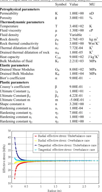
Fig. 2: Case history: Tangential and radial effective stress variation

Field case-results: The developed stability analyses considered an “overbalanced case” characterized by a mud pressure applied to wellbore wall, pw, very close to formation pressure po and an “underbalanced case” in which pw was set equal to 0.85 po.

The input data used to describe the thermodynamic, petrophysical and elastoplastic behavior of the shaly-sand formation are summarized in Table 1.

As far as the geometrical discretization is concerned, the spatial investigation domain extended from the borehole radius, set equal to 0.1 m, to the

Fig. 3: Case history: Tangential and radial strain variation

Fig. 4: Case history: Radial displacement variation in overbalance and underbalance cases

external boundary, equal to 30 m and it was divided into 54 grid elements. The temporal evolution of phenomena was analysed 24 h after drilling operations. For the initial conditions the values of the natural in situ stress, pore pressure and temperature typical of a 2000 m deep formation, characterized by normal geostatic and geothermal gradients, were imposed. The stress domain was set isotropic on the horizontal plane and characterised by a horizontal vs. vertical stress ratio equal to 0.76. As far as the boundary conditions are concerned, the boundary values were imposed equal to the natural initial conditions at the external investigation radius, whereas the boundary values set at the wellbore wall reproduced the drilling thermodynamic and stress conditions.

(9)

Fig. 5: Case history: Radial and tangential effective stress variation (overbalance cases)

Figure 2 and 3 show that adopting an overbalance technique, the magnitude of radial and tangential stresses (and, obviously, of the relative radial and tangential strains) induced by drilling operations into the formation, was not so large as to compromise wellbore safety. The application of the Mohr-Coulomb yield criteria confirmed the stability of the investigated reservoir strata under overbalance drilling conditions. On the other hand, if the hydrostatic pressure in the circulating downhole fluid system during drilling was maintained at a pressure lower than the pressure of the target formation (“underbalanced case”), the stress increment induced into the rock would compromise wellbore safety. For the drilling approach which was identified as the best solution, i.e., the overbalanced case, the temporal evolution of phenomena was analysed not only immediately after the wellbore drilling (24 h), but also twenty days after drilling operations, when a new equilibrium was achieved into the formation. The results in Fig. 4 and 5 shows that the geomechanical and thermodynamic temporal variations are fully compatible with wellbore safety.

CONCLUSION

The adoption of a borehole instability modelling approach is fundamental when addressing technical and safety issues related to any drilling, completion and extraction design phase because it permits a systematic consideration of the stress variations around the borehole and the associated rock deformations and pore pressure changes.

The importance of adopting of a coupled thermo-dynamical/geomechanical theory for an accurate investigation of the complex behavior of many rock formations encountered while drilling is widely accepted and the definition of a numerical solution

suitable for such complex coupled multi-physical theory implementation is anything but trivial.

In this study the numerical solution developed for implementing Charlez’s thermo-porous-elastic-plastic theory, where plasticity is described by the basic Desai’s model, is presented.

The adoption of a fully coupled approach allows porous flow, temperature development and rock deformation calculations to be performed together. The method is also called implicit coupling since the whole system is discretised on one grid domain and solved simultaneously for both the thermodynamic variables and the geomechanical response. This approach has the advantage of internal consistency and stability; moreover, it preserves second order convergence of nonlinear iterations. Furthermore, in order to implement the plastic analysis, an iteratively coupled approach was adopted inside the fully coupled routine. According to the iterative coupling technique, the model basic equations and the plastic behavior equations are solved separately and sequentially at each non-linear iteration. This was achieved by solving two nested Newton-Raphson cycles at each time-step. The iterative coupling approach corresponds to an implicit treatment of the plastic variables, essential to preserve the stability of the elastic-plastic solution.

Application of the proposed approach to synthetic and real cases showed the value and potential impact on economical and safety issues of wellbore drilling.

ACKNOWLEDGEMENT

The researcher wishes to acknowledge Prof. Verga for her invaluable contribution to this study.

REFERENCES

1. Charlez, A., 1991 Rock Mechanics. Theoretical fundamentals. t editions technip. ISBN: 2-7108-0585-5, pp: 360.

2. Coussy O.,1995 Mechanics of Porous Continua. John Wiley and Sons Ltd., ISBN: 0471952672, pp: 472.

3. Dean, R.H., X. Gai, C.M. Stone and S.E. Minkoff, 2003. A comparison of techniques for coupling porous flow and geomechanics. Proceeding of the SPE Reservoir Simulation Symposium, Feb. 3-5, SPE, Houston, Texas, USA., pp: 1-9. DOI: 10.2118/79709-PA

(10)

5. Desai C.S. and Q.S.E. Hashmi, 1989. Analysis, evaluation and implementation of a nonassociative model for geologic materials. Int. J. Plastic., 5: 397-420.

6. Desai, C.S., 1980. A general basis for yield, failure and potential functions in plasticity. Int. J. Numer. Anal. Methods Geomech., 4: 361-375.

7. Desai, C.S., S. Somasundaram and G. Frantziskonis, 1986. A hierarchical approach for constitutive modeling of geologic materials. Int. J. Numer. Anal. Methods Geomech., 10: 225-257.

8. Rocca, V. and F. Verga, 2008. Stability modelling applied to wellbore design. GEAM. Geoingegneria Ambientale E Mineraria, XLV: 5-12.

9. Rocca, V., F. Verga, M. Cesaro, G. Maletti and F. Zausa, 2006. Application of Desai’s Model for Borehole Stability Analyses in Shale Formations. In: Mine Planning and Equipment Selection 2006, Cardu, M. et al. (Eds.). GEAM, ISBN: 88-901342-4-0, pp: 1279-1284.

10. Sartori, L.,1994. Analisi e proposte per la formulazione termo-poro-elasto-plastica. Relazione tecnica n. 2. ENI SpA-E andP Division internal report.

11. Settari, A. and D.A. Walters, 1999. Advances in couplet geomechanical and reservoir modeling with applications to reservoir compaction. Proceeding of the SPE Reservoir Simulation Symposium, Feb. 14-17, Society of Petroleum Engineers Inc., Houston, Texas pp: 1-13. DOI: 10.2118/51927-MS

12. Tran, D., A. Settari and L. Nghiem, 2002. New iterative coupling between a reservoir simulator and a geomechanics module. Proceeding of the SPE/ISRM Rock Mechanics Conference, Oct. 20-23, Society of Petroleum Engineers Inc., Irving, Texas, pp: 1-10. DOI: 10.2118/78192-MS