Article
Printed in Brazil - ©2016 Sociedade Brasileira de Química 0103 - 5053 $6.00+0.00
*e-mail: [email protected]
Fighting Collinearity in QSPR Equations for Solution Kinetics with
the Monte Carlo Method and Total Weighting
Ruben A. Elvas-Leitão*,a,b
aÁrea Departamental de Engenharia Química, Instituto Superior de Engenharia de Lisboa, Instituto
Politécnico de Lisboa, R. Conselheiro Emídio Navarro, 1959-007 Lisboa, Portugal
bCentro de Química e Bioquímica, Ed. C8, Campo Grande, 1749-016 Lisboa, Portugal
A Monte Carlo method is used in addition to functional and individual weighting to overcome multicollinearity problems in multiple linear regression equations applied as quantitative-structure-property-relationships, allowing the estimation of correct coefficient confidence intervals. The method was applied to rate constants for the Menschutkin reaction between Et3N and EtI in mono- and di-alcohols, at 25.00 ºC. Results show that the use of our methodology produces a significant improvement upon confidence interval estimates regardless of the level of collinearity present. Addition of weighting shows additional advantages, increasing the overall consistency of the regression process.
Keywords: Monte Carlo, multicollinearity, correlation, MLR
Introduction
The search for quantitative structure-property relationships (QSPR) to interpret and predict solvent effects upon reaction rates often resorts to linear model equations, of the general form,
ln k = f(x1, x2,…, xn) (1)
where k stands for rate constant and xn is a descriptor of a
given type of substrate-solvent or solvent-solvent interaction. Early models included just one or two descriptors but it is now well established that, in general, four descriptors are needed to account for the main physicochemical features underlying the reaction process. These descriptors include Lewis acidity and basicity, dipolarity/polarizability and also a cavity term related to the work needed to form a cavity to accommodate the substrate.1,2
Over the years a large number of solvent descriptors have been proposed to describe substrate-solvent interactions, some based on macroscopic properties such as dielectric constant, dipole moment and refractive index and others on microscopic properties, usually obtained from probes showing spectroscopic shifts due to different solvent effects upon the signal-wave number (UV-Vis and infrared (IR))
or chemical shift (nuclear magnetic resonance (NMR)).3-5
Subsequently, several multiparametric model equations corresponding to different combinations of descriptors have been used, leading to a greater understanding of the type of interactions present and their effect upon the rate of a given reaction, thus providing useful mechanistic clues and, most of all, generating sound equations to accurately predict rate constants for similar reactions.5
The most useful method to obtain this information has been found to be multiple linear regression (MLR). Ideally, from a mathematical point of view, any descriptors in a given MLR model equation should be orthogonal to each one of the others and, desirably, also to their linear combinations threshold values being, respectively, r2 > 0.5
and R2 > 0.8.6 However, more often than not, they present
significant degrees of collinearity, especially when only a closely related set of solvents is used, e.g., a set of monoalcohols, and/or small variabilities are observed for the chosen descriptors, within the data set.
In general, this fact does not affect significantly regression coefficients, except in cases where descriptors present high correlation coefficients. Even when collinearity does not affect regression coefficients, consequences of collinearity become apparent through the often inflated magnitude of coefficient uncertainties, σi, whose values
coefficients (CIi), can subsequently be calculated through
the use of t-values for the chosen confidence level (e.g.,68, 95, or 99%), according to,
CIi = ±tσi (2)
CIs are particularly important, for interpretative and predictive purposes, especially if one aims to interpolate reliable estimates of predicted k values.7
A number of methods proposed over time (principle component analysis, factor analysis, etc.) although successful in overcoming this problem, are more difficult to apply and change the descriptors’ structure in their effort to orthogonalize descriptors’ axes, leading to solutions that frequently bear unclear physical meaning and make interpretation of results difficult if not impossible. Other techniques such as ridge regression produce unbiased estimates of parameters, but their expected values are not at all equal to the true values. Generally, they tend to be underestimated (sometimes grossly) even if the variance of these estimates can be so much lower than that of the least-squares estimator and, of course, the total expected mean squared error is also less, which makes it (in a certain sense) a “better” estimator for some but surely not all intended purposes.8
Monte Carlo (MC) methods, on the other hand, are rather less known as an efficient method for dealing with the type of problem here addressed, although they are widely used in computer simulations. Unlike parametric statistics, they require no assumptions about the distribution of uncertainties or the collinearity among variables, thus allowing calculation of reliable coefficients and their confidence intervals.9-12
The Monte Carlo method assumes that the data set is a sample of all possible sets, randomly drawn by the experimental method within experimental uncertainty. Using this procedure one can simulate as many synthetic data sets as one needs (n), drawn from a particular model, just by introducing the appropriate random noise (δi):
ki’ = ki + δi (3)
Random numbers are generated using any algorithm that can ensure long non-repeating sequences with the appropriate standard deviation and zero mean value. Usually, since it is assumed that coefficient uncertainties follow a Gaussian distribution, the generated numbers are normally distributed in order to later allow the calculation of confidence intervals for each equation parameter. Each synthetic data collection is then subjected to a regression analysis leading to n “synthetic” parameter sets (a1, a2,..., an), (b1, b2,..., bn), etc.12
Alternatively, using the method proposed by Alper and Gelb,9,10 confidence intervals (given from the adequate
number of computer runs) can be easily and accurately calculated without the usual assumption of normality for uncertainty distribution by the simple exclusion of the appropriate number of high and low solution values from the generated sets by ordering the calculated values and excluding the (100 – x)% / 2 top and bottom ones, thus obtaining x% CIs. The minimum number of sets to be generated for each confidence level has also been established by these authors.
Finally, another usual MLR assumption is that uncertainties for the whole experimental data set are equal. In reality experimental results may have very different standard deviations (σi). In this instance, it is a well-known
(but scarcely used) practice to use individual correcting weights (wi). This type of individual weighting accounts
for the accuracy of each value and, in most situations, it is considered to be inversely proportional to σi2, the variance
of each set of replicate measurements, or the estimate of a single measurement.13,14
In the case of kinetic measurements, the accuracy of ki
values may vary significantly due to experimental errors and especially if values from different authors and/or different measurement techniques have been used.
Much more uncommon, in the same context, is the use of global weighted regression to correct for effects due to transformations on the dependent variable, although this regression tool has been clearly shown to contribute towards correcting these same effects, mainly when significant compression/expansion of uncertainties is present as is the case with logarithms.14-21
For a logarithmic transformation such as Yi = ln (ki), the
original assumption is, again, that ki values are normally
distributed, but we are actually minimizing the sum of squares of the deviations in ln (ki), and these do not follow a
Gaussian distribution, since there is a compression of the data for low ki values and an expansion for the higher ones.16-19
When experimental ki values are converted to Yi (e.g.,
ln k, 1 / k), assuming the usual hypothesis that ∆Yi and ∆ki
are relatively small, we can write, following de Levie,18
(4)
The global weighting factor (w'i) dictated by the
mathematical transformation of the data, is given by,
In the present case, the transformation of the rate constant (ki) into ln (ki) yields,
(6)
Both types of weighing factors should be used together: their combination (Wi), the total weight, is achieved by
multiplying the two weighing factors. In the present case, this produces the expression,
(7)
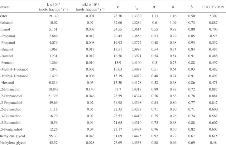
In this paper, we show the advantages of the combined use of these methodology changes in multiparametric QSPR applied to kinetics, through its application to a data set of 20 rate constants for the Menschutkin reaction of Et3N with EtI in mono- and di-alcohols at 25.00 ºC
(Table 1) that were previously correlated with two sets of four solvent descriptors from two multiparametric QSPR
models by Calado et al.22 In this work, the authors applied
two suitable models to their experimental data set, one predominantly solvatochromic, the Taft-Abboud-Kamlet-Abraham equation (TAKA),23 and one based prevalently
on macroscopic descriptors, the Gonçalves-Albuquerque-Simões equation (GAS).24
For the TAKA equation we have
ln k = a0 + a1π* + a2α + a3β + a4C (8)
where the solvatochromic descriptors are π*, a measure of
the solvent’s dipolarity/polarizability; α and β which are, respectively, measures of the solvent’s ability to donate (Lewis acidity) or accept (Lewis basicity) a hydrogen bond from a given substrate; and C which is the cohesive energy density, a macroscopic descriptor intended to measure the solvent’s contribution to the formation of a cavity to harbor the substrate’s molecule.
For the GAS equation we have
ln k = a0 + a1f(ε) + a2g(nD) + a3ETN + a4C (9)
In this equation, f(ε) is the Kirkwood function of
Table 1. Rate constants (k) for the reaction of Et3N with EtI and select solvent properties at 25.00 ºC19
Solvent k × 10
5 /
(mole fraction-1 s-1)
σ(k) × 105 /
(mole fraction-1 s-1) ε nD π
* α β C × 10-3 / MPa
Water 191.40 0.001 78.30 1.3330 1.13 1.16 0.50 2.307
Methanol 10.02 0.07 32.66 1.3284 0.6 1.09 0.73 0.887
Ethanol 5.151 0.009 24.55 1.3614 0.55 0.88 0.80 0.703
1-Propanol 2.686 0.012 20.45 1.3856 0.53 0.79 0.85 0.59
2-Propanol 4.079 0.008 19.92 1.3772 0.48 0.68 0.93 0.552
1-Butanol 1.968 0.017 17.51 1.3993 0.54 0.74 0.84 0.485
2-Butanol 3.231 0.012 16.56 1.3971 0.54 0.54 0.91 0.488
1-Pentanol 1.269 0.010 13.9 1.4100 0.5 0.73 0.88 0.497
2-Methyl-1-butanol 1.047 0.002 15.63 1.4088 0.51 0.64 0.93 0.482
3-Methyl-1-butanol 1.429 0.006 15.19 1.4072 0.48 0.74 0.91 0.497
1-Hexanol 0.819 0.03 13.30 1.4178 0.52 0.68 0.86 0.471
1,2-Ethanediol 18.842 0.140 37.7 1.4318 0.89 0.88 0.72 0.887
1,2-Propanediol 21.393 0.046 28.59 1.4324 0.76 0.83 0.78 0.881
1,3-Propanediol 49.69 0.02 34.98 1.4398 0.84 0.80 0.77 0.847
1,2-Butanediol 11.16 0.05 22.35 1.4378 0.71 0.80 0.71 0.600
1,3-Butanediol 16.70 0.02 28.57 1.4410 0.75 0.76 0.74 0.562
2,3-Butanediol 10.56 0.04 21.65 1.4310 0.75 0.68 0.88 0.602
1,5-Pentanediol 12.26 0.04 27.17 1.4494 0.76 0.70 0.82 0.603
Diethylene glycol 55.33 0.043 31.69 1.4475 0.92 0.72 0.67 0.615
Triethylene glycol 45.52 0.028 23.69 1.4558 0.88 0.66 0.69 0.48
k: rate constant; ε: relative permittivity; nD: refractive index; π*: TAKA dipolarity/polarizability parameter; α: TAKA Lewis acidity parameter; β: TAKA
the relative permittivity; ε relates to dipolarity; g(nD) is
a function of the refractive index; nD measures the
polarizability effect; ETN is the normalized Dimroth and
Reichardt parameter and measures a blend of dipolarity and Lewis acidity effects; and C has the same meaning as above.
Methodology
The procedure used was as follows: (i) classical regression was performed over the experimental data using a correlation equation to determine a set of coefficients; (ii) each ki value was scattered by adding a random
number, δi (equation 3), to construct a new “experimental”
mathematical solution; (iii) the resulting MC data set was analyzed through classical regression and a new set of coefficients was obtained; (iv) this sequence was repeated n times, where n is the necessary total number of synthetic data sets; and (v) the CI for each coefficient was obtained as described above by ordering the coefficient values and excluding the (100 – 68)% / 2 top and bottom ones.
The computational conditions were chosen using Alper and Gelb’s criteria;9,10 therefore, since we chose to
use 68% confidence intervals (ca. 1σ), the number of MC simulations, n, equaled 200. Normally distributed random uncertainty was introduced through a routine written before. The number set had µ = 0 and σ = 1.5 × 10⁻⁴.
This latter value for the standard deviation can be considered as a scattering factor. It is usually chosen from information on the magnitude of the uncertainties affecting the dependent variable. In the present study, a different approach, previously developed by us,
was used:17 using the TAKA equation in each
mono-descriptor reduced form, where no collinearity problems can be present, the standard deviation of the random uncertainty numbers set was adjusted by repeating the MC procedure with different scattering factors until the averaged coefficients’ confidence intervals were identical to those calculated through classical regression. The same scattering factor was then used for equations 7 and 8. This procedure has avoided the need for previous knowledge or pre-assumption of a given uncertainty level.
Goodness-of-fit has been analyzed in terms of the standard deviation of the fit (σfit), defined in the usual
manner,
(10)
where n is the number of data points, p is the number of
equation parameters and Wi is the total weighting which
is equal to unity if none of the weighting types are used.
Results and Discussion
The degree of collinearity among equation descriptors has been determined in terms of the determination coefficient (r2) (Tables 2 and 3), showing that several
descriptors are highly correlated in both models.
The correlation of each descriptor with linear combinations of pairs of the remaining descriptors (Tables 4 and 5) is also above the limit (R2 > 0.8) in several cases.
Results above are not surprising since the observed multicollinearity is mostly a result of studying a specific family of solvents. Nevertheless, the best equations’ subsets were the same for the classical and Monte Carlo methods.
Regarding the best equation for the TAKA model, the stepwise regression method indicates that only π* is
significant, i.e.,
ln k = a0 + a1π* (11)
and therefore this model will be used only to show the strict equivalence of results for the two approaches, as can be seen in Table 6 in which the comparison of results between classical regression and the MC method for equation 11 Table 3. Correlation among variables in equation 9
r2 f(ε) g(n
D) ET
N C
f(ε) 1 0.0108 0.7952 0.6843
g(nD) – 1 0.0423 0.0430
ETN – – 1 0.7576
C – – – 1
r2: determination coefficient; f(ε): Kirkwood function of the relative
permittivity; g(nD): function of the refractive index; ETN: normalized
Dimroth and Reichardt parameter; C: cohesive energy density.
Table 2. Correlation among variables in equation 8
r2 π* α β C
π* 1 0.1930 0.7513 0.4487
α – 1 0.4861 0.6398
β – – 1 0.5425
C – – – 1
r2: determination coefficient; π*: TAKA dipolarity/polarizability
shows only very small differences in the confidence intervals and no difference in σfit.
Table 7 depicts the results for the GAS model, for which the best equation is:
(12)
Results clearly indicate that, although the coefficients obtained in both cases are similar, the use of the Monte Carlo method leads to significantly less conservative estimates of the coefficients’ confidence intervals, with relative differences ranging from –26 to –64%. The MC fit itself shows a somewhat larger standard deviation but with no statistical significance (the F-test on variances confirmed that they are equal up to a significance level of 98%).
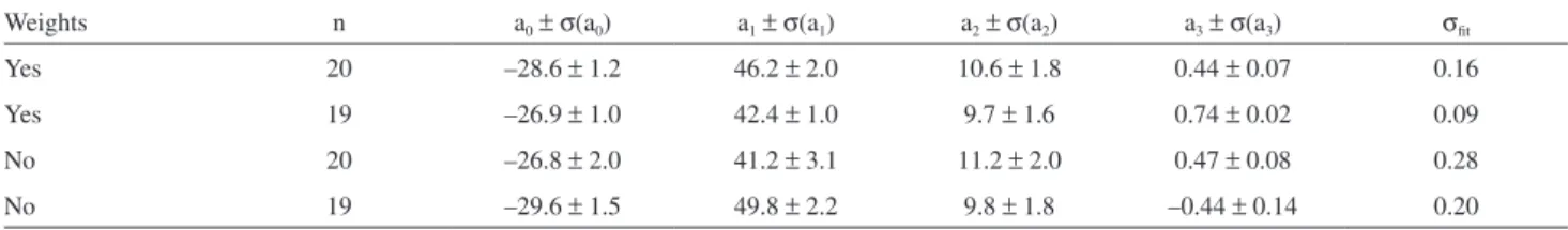
The effect of weighting in addition to the use of the MC method is shown in Table 8, along with the same effects on a subset that excludes water.
On one hand, it is clear from the 1st and 3rd rows that
the use of weights improves regression results, as can be perceived through σfit values. Furthermore, global
weighting also increases the internal consistency of the tested data set: if one uses non-weighted regression, the comparison of results for the original data set (20 points) and a subset excluding water shows a change on the Table 4. Correlation between each variable in equation 8 and linear
combinations of two of the remaining variables
R2 β + α α + C C + β
π* 0.8043 0.4745 0.7535
π* + β π* + C C + β
α 0.5956 0.6566 0.6653
π* + α α + C π* + C
β 0.8754 0.5749 0.7954
α + β π* + β π* + α
eC 0.7020 0.5464 0.7654
R2: multiple determination coefficient; π*: TAKA dipolarity/polarizability
parameter; α: TAKA Lewis acidity parameter; β: TAKA Lewis basicity parameter; C: cohesive energy density.
Table 5. Correlation between each variable in equation 9 and linear combinations of two of the remaining variables
R2 g(n
D) + ET
N g(n
D) + C ET N + C
f(ε) 0.8954 0.7364 0.9063
f(ε) + ETN f(ε) + C ETN + C
g(n
D) 0.0731 0.3583 0.4450
f(ε) + C g(nD) + f(ε) g(nD) + C
ETN 0.9122 0.8080 0.8054
g(nD) + f(ε) f(ε) + ETN g(n D) + ETN
C 0.6538 0.7712 0.7376
R2: multiple determination coefficient; f(ε): Kirkwood function
of the relative permittivity; g(nD): function of the refractive index;
ETN: normalized Dimroth and Reichardt parameter; C: cohesive energy
density.
Table 6. Comparison between classical and Monte Carlo methods for equation 11
Method Weights a0±σ(a0) a1±σ(a1) σfit
Classical No –6.37 ± 0.21 3.33 ± 0.30 0.232
Monte Carlo No –6.37 ± 0.23 3.33 ± 0.28 0.232
an±σ(an): coefficient confidence interval; σfit: standard deviation of the fit.
Table 7. Comparison between classical and Monte Carlo methods for equation 12
Method Weights a0±σ(a0) a1±σ(a1) a2±σ(a2) a3±σ(a3) σfit
Classical No –26.4 ± 2.7 41.4 ± 6.4 10.9 ± 3.2 0.48 ± 0.22 0.22
Monte Carlo No –26.8 ± 2.0 41.2 ± 3.1 11.2 ± 2.0 0.47 ± 0.08 0.28
∆σ / % –26 –53 –38 –64 –
ai±σ(ai): coefficient confidence interval; σfit: standard deviation of the fit.
Table 8. The effect of weighting, using the MC approach, on the original data set and on a subset excluding water for equation 12
Weights n a0±σ(a0) a1±σ(a1) a2±σ(a2) a3±σ(a3) σfit
Yes 20 –28.6 ± 1.2 46.2 ± 2.0 10.6 ± 1.8 0.44 ± 0.07 0.16
Yes 19 –26.9 ± 1.0 42.4 ± 1.0 9.7 ± 1.6 0.74 ± 0.02 0.09
No 20 –26.8 ± 2.0 41.2 ± 3.1 11.2 ± 2.0 0.47 ± 0.08 0.28
No 19 –29.6 ± 1.5 49.8 ± 2.2 9.8 ± 1.8 –0.44 ± 0.14 0.20
sign associated with a3. However, a similar comparison
for the weighted regression shows an alteration on the magnitude of a3 but with the sign remaining unchanged.
This apparently small difference is rather significant in terms of both interpretation and prediction.
It is also easily seen that the uncertainties affecting each k value are generally very small when compared with the residuals of each fit, causing the chi-square of each fit to become larger than the number of degrees of freedom in all cases (a “rule of thumb” indicates that they should be close).12 This is a common situation in this type of context
and is due probably to the empirical or semi-empirical nature of solvent descriptors and to the formal procedure of considering the mere additivity of all included effects.
Conclusions
From the above analysis, we can conclude that the proposed MC method, especially when combined with global weighting, allows a significant improvement on the calculation of uncertainties on MLR coefficients, and increases the overall consistency of the regression process otherwise affected by the presence of multicollinearity. The interpretation and/or prediction process becomes, therefore, more reliable.
Supplementary Information
Supplementary information (Pascal code for MC confidence interval estimation) is available free of charge at http://jbcs.sbq.org.br as PDF file.
Acknowledgments
Financial support by Fundação para a Ciência e Tecnologia, Portugal, under Projects PEST OE/QUI/ UI10612/2013 and PEST UID/MULTI/00612/2013 is greatly appreciated.
References
1. Koppel, I. A.; Palm, V. A. In Advances in Linear Free Energy Relationships; Chapman, N. B.; Shorter, J., eds.; Plenum Press: New York, 1972, ch. 5.
2. Kamlet, M. J.; Abboud, J.-L. M.; Abraham, M. H.; Taft, R. W.;
Prog. Phys. Org. Chem. 1981, 35, 485.
3. Politzer, P.; Murray, J. S. In Quantitative Treatments of Solute/ Solvent Interactions; Politzer, P.; Murray, J. S., eds.; Elsevier: New York, 1994, ch. 1.
4. Abboud, J.-L. M.; Notario, R.; Pure Appl. Chem. 1999, 71, 645. 5. Reichardt, C.; Welton, T.; Solvents and Solvent Effects in
Organic Chemistry, 4th ed.; Wiley-VCH: Weinheim, 2011.
6. Martins, F.; Santos, S.; Ventura, C.; Elvas-Leitão, R.; Santos, L.; Vitorino, S.; Reis, M.; Miranda, V.; Correia, H. F.; Aires-de-Sousa, J.; Kovalishyn, V.; Latino, D. A. R. S.; Ramos, J.; Viveiros, M.; Eur. J. Med. Chem.2014, 81, 119.
7. Milton, J. S.; Arnold, J. C.; Probability and Statistics in the
Engineering and Computing Sciences; McGraw-Hill: New
York, 1986.
8. Livingstone, D.; Data Analysis for Chemists; Oxford University Press: Oxford, 1995.
9. Alper, J. S.; Gelb, R. I.; J. Phys. Chem.1990, 94, 4747. 10. Alper, J. S.; Gelb, R. I.; Talanta1993, 40, 355.
11. Press, W. H.; Flannery, B. P.; Teukolsky, S. A.; Vetterling, W. T.; Numerical Recipes in Pascal; Cambridge University Press: Cambridge, 1989.
12. Buckland, S. T.; Biometrics1984, 40, 811. 13. de Levie, R.; J. Chem. Educ.1986, 63, 10.
14. Bevington, P. R.; Data Reduction and Error Analysis for the
Physical Sciences; McGraw-Hill: New York, 1969.
15. Kalantar, A. H.; J. Phys. Chem.1986, 90, 6301. 16. Shatkay, A.; Azor, M.; Anal. Chim. Acta1981, 133, 183. 17. Gonçalves, R. M. C.; Martins, F. E. L.; Leitão, R. A. E.; J. Phys.
Chem.1994, 98, 9540.
18. de Levie, R.; Advanced Excel for Scientific Data Analysis; Oxford University Press: New York, 2004
19. Tellinghuisen, J.; J. Phys. Chem. A2000, 104, 11829. 20. Sung, D. D.; Kim, J. Y.; Lee, I.; Chung, S. S.; Park, K. H.; Chem.
Phys. Lett.2004, 392, 378.
21. Bolster, C. H.; Tellinghuisen, J.; Soil Sci. Soc. Am. J.2010, 74, 760.
22. Calado, A. R. T.; Pinheiro, L. M. V.; Albuquerque, L. M. P. C.; Gonçalves, R. M. C.; Rosés, M.; Ràfols, C.; Bosch, E.; Collect.
Czech. Chem. Commun.1994, 59, 898.
23. Abraham, M. H.; Doherty, R. M.; Kamlet, M. J.; Harris, J. M.; Taft, R. W.; J. Chem. Soc., Perkin Trans. 21987, 913. 24. Gonçalves, R. M. C.; Simões, A. M. N.; Albuquerque, L. M. P.
C.; J. Chem. Soc., Perkin Trans. 21990, 1379.