A Work Project presented as part of the requirements for the Award of a Masters Degree in Economics from the NOVA - School of Business and Economics and Insper It takes more than soccer to make Argentinians, Brazilians, Chileans and Mexicans happy

(1)

A Work Project presented as part of the requirements for the

Award of a Masters Degree in Economics from the NOVA -

School of Business and Economics and Insper

It takes more than soccer to make Argentinians, Brazilians,

Chileans and Mexicans happy

Patricia Ferraz Regula - Student #769

A Project carried out under the supervision of:

Professor Regina Carla Madalozzo (Insper

–

BR)

Professor Paulo M. M. Rodrigues (Nova

–

PT)

(2)

This dissertation explores the socioeconomic determinants of happiness for Argentinians, Brazilians, Chileans and Mexicans, and analyzes its evolution over the years and between these countries. The analysis in this dissertation is based on the World Value Survey waves 2, 3 and 5. With this data it was possible to analyze and compare the determinants that are most relevant for these populations to self-declare themselves as happy. Determinants such as social class, education, employment, among others, showed significance in some years for some populations and were found not significant for others. Health, religion and national pride were the most consistent, always pointing in the same direction and at least statistically significant in one of its categories.

(3)

1

.

Introduction ... 3

2. Data analysis ... 7

3. Methodology ... 9

4. Results ... 11

5. Conclusion ... 21

6. Appendix ... 23

(4)

1. Introduction

Happiness is a very complex sentiment which Halliwell et al. (2012) have divided

into two spheres: the first is emotional, related to friendship, family, day-to-day work; and the other is cognitive, encompassing personal and professional satisfaction, health

and all human frustrations and satisfactions. In general “Being Happy” is a frequently

given answer when people are asked what they wish for their lives, and this answer is based on these two spheres. However, what does make people happy and under what conditions is a person considered happy? Does happiness only depend on the individual and the choices he/she makes in life or is it affected by the environment the individual lives in, by the conditions of life individuals have and the country he/she lives in?

One of the first researchers of this subject was Aristotle, who, in his best-known work

on ethics, Nicomachean Ethics, indicates that “Happiness is a first principle; for it is for

the sake of this we all do all the rest of our actions, and the first principle and cause of goods we take to be something honourable and divine” (ARISTOTLE, 2000, p.20). In a

recent psychology study Seligman (2002) proposed a division of happiness into three components: the first is associated to pleasure and gratification; the second is associated to embodiment of strengths and virtues, having a good life with work, friends and family; and the third is related to meaning and purpose, have something to believe in and contribute for.

(5)

When analyzing happiness of a country we have to take into consideration that each individual has its own preferences, and not only are these personal, but they are not comparable between individuals, i.e., many times what makes one person happy will not

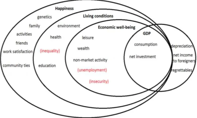
necessarily make another person happy as well. In 2006, a Deutsche Bank report1 revealed

more than 15 factors that influence the happiness and well-being of a population; these factors are not only economic, but social and personal as well. Some of these factors will be explored throughout this paper.

Figure 1: Components of well-being and happiness

Source: author, based on Deutsche Bank (2006)

To produce this study a Word Value Survey (WVS) database was used. This database results from a global research that has been conducted since 1981 and that explores the values and behavior of people across different countries. The waves considered in this study are Wave 2 (1991-1993), Wave 3 (1996-1998) and Wave 5 (2005-2007). Four Latin American countries are analyzed (Argentina, Brazil, Chile and Mexico) based on the three different waves, with the goal of identifying the factors that have the

1_Available _at _{http://www.dbresearch.com/PROD/DBR_INTERNET_EN-PROD/PROD0000000000202587.PDF}

(6)

biggest impact on happiness and how they behave over time. Answers associated to social class (income), health, group age, civil status and religion were used to understand the determinants that lead an individual to be or to self-declare him/herself as happy.

Easterlin (1974) concluded that income is directly linked with happiness, but overtime this linkage stops being valid. In the countries studied by Easterlin, people with higher income were self-declared happier than people with lower income, but when the comparison was conducted between countries the linkage between income and happiness was not different, even between countries with a substantial income difference.

Pukeliene and Kisieliauskas (2013) concluded that individuals of developed countries are more likely to be happy than those in developing countries. However, the four developing countries that were studied are among the 30 happiest of the world according to “The United Nations General Assembly's second World Happiness Report”

(2013). Mexico is the happiest of all four, taking up the 16th position, followed by Brazil (24th), Chile (28th) and Argentina (29th). Pukeliene and Kisieliauskas (2013) concluded also that in 11 of the 21 countries analysed there is a strong to mild relationship between income and well-being.

For Latin America, Corbi and Menezes-Filho (2005) examined the empirical determinants of happiness in Brazil using Wave 3 of the WVS and concluded that people with higher income and with a job tend to be happier. A recent study by Tetaz (2012), also using the WVS database, showed that for Argentina income is not always a relevant determinant of happiness, e.g., for the capital Buenos Aires, it was only relevant during the year of 2006.

(7)

were only analyzed in the papers mentioned above and for Mexico and Chile, no country-specific references have been found.

Another theme that is often questioned by sceptical economists when discussing happiness is the existence of causality of the employed variables, e.g., healthy people are happier or happy people are healthier. Cheah and Tang (2013) showed that, for instance in Malaysia, variables associated to health, education and civil status influence local happiness. Furthermore, Cheah and Tang showed that being employed does not have an influence on happiness, probably because with more time to spare happiness is found in different ways, e.g. spending more time with family.

Variables such as religion and national pride were not yet well explored in other papers and, therefore, are considered in our analysis. All other variables that were already

proved relevant in other studies, such as income2, health, and education are also used in

this study.

The remainder of the dissertation is organised as follows. Section 2 introduces the description and analyzes the database used. In section 3, the methodology is described and in section 4 the results obtained are discussed. Finally, in section 5 the main conclusions of this dissertation will be presented and suggestions for follow-up studies and research in this field will be pointed out.

2_{Most studies make use of income (divided into 10 categories by WVS) as a financial variable, however, when}

(8)

2. Data analysis

The Word Value Survey (WVS) is, along with the Latinobarómetro, one of the most important indicators regarding well-being and behavior for Latin America. Divided into waves (every two or three years), the WVS is carried out since 1981 and has worldwide reach. For this dissertation we will use waves 2, 3 and 5, because the countries subject to this study are present in all three, enabling a direct comparison between them. Given the extension of the survey, over two hundred questions, not all questions were used due to relevance.

Since data from three different waves was used and these have a gap of 15 years between the oldest (wave 2) and the most recent (wave 5), some data had to be adjusted in order to allow for comparison, but maintaining fidelity to the original source and the overall theme of the questions and answers. Below is the distribution of the answer for the happiness question for the four countries and the three different waves. The answer

has four different alternatives: “Not at all happy”, “Not very happy”, “Quite happy”,

“Very happy”. Below we have the distribution for the answers “Not very happy”3 and “Very happy”.

Table 1: Happiness by age group – WVS wave 2, wave 3 and wave 5

3_{The classification “Not at all happy” was not used in this comparison since the portion of people self}_-_{declared “Not}

at all happy” is too small. Instead, to make the comparison easier, the category “Not very happy” was used as

replacement.

Argentina

Wave 2 (1991) Wave 3 (1995) Wave 5 (2005)

Happiness level Not very

happy Very happy

Not very

Age group % % % % % %

18-24 years old 11.95% 35.85% 15.85% 32.24% 6.08% 38.12%

25-34 years old 14.98% 36.71% 14.16% 28.76% 9.02% 36.07%

35-44 years old 18.58% 34.43% 14.92% 28.86% 13.95% 31.40%

45-54 years old 21.43% 33.33% 15.62% 30.00% 11.65% 34.25%

(9)

Source: author, based on World Value Survey

From the analysis of the data in table 1, an improvement of the happiness sentiment for all countries analyzed is observed between wave 2 and wave 5, but mainly among the younger groups. Hence, it is possible that the perception of well-being of people improved in these countries. When analyzing Brazil and Mexico, beyond the drop

in the volume of people self-declared as “Not very happy”, an increase of people

self-declared as “Very happy” is observed, which can lead us to think that in these countries

Brazil

Wave 2 (1991) Wave 3 (1997) Wave 5 (2006)

Not very

Age group % % % % % %

18-24 years old 23.92% 17.77% 16.36% 21.09% 8.33% 43.33%

25-34 years old 23.20% 17.60% 17.02% 24.92% 9.50% 34.56%

35-44 years old 22.66% 19.63% 14.17% 22.50% 8.57% 32.06%

45-54 years old 24.14% 24.14% 12.65% 18.67% 9.80% 30.59%

+55 years old 16.29% 25.31% 13.00% 19.00% 9.31% 30.00%

Chile

Wave 2 (1990) Wave 3 (1996) Wave 5 (2005)

Not very

Age group % % % % % %

18-24 years old 23.97% 34.07% 16.75% 27.75% 8.77% 42.69%

25-34 years old 20.54% 33.42% 16.10% 27.34% 11.89% 35.27%

35-44 years old 24.05% 35.74% 17.35% 29.08% 14.35% 33.49%

45-54 years old 25.13% 31.79% 18.37% 23.53% 22.36% 25.47%

+55 years old 33.78% 31.08% 25.71% 29.52% 22.31% 29.23%

Mexico

Wave 2 (1990) Wave 3 (1996) Wave 5 (2005)

Not very

Age group % % % % % %

18-24 years old 24.35% 25.77% 24.12% 32.92% 6.06% 60.60%

25-34 years old 25.71% 29.19% 32.01% 26.25% 5.62% 64.87%

35-44 years old 27.20% 24.40% 29.15% 27.25% 8.17% 59.48%

45-54 years old 32.65% 28.57% 29.79% 23.29% 9.16% 59.16%

(10)

the quality of live improved substantially. Still, the question remains: Has such an improvement actually occurred?

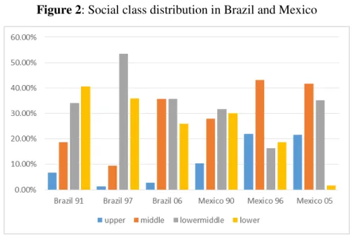
Paying particular attention to these two countries – Brazil and Mexico – and evaluating the social class variable (Figure 2), it is possible to notice that, at first, there is a direct and growing relationship between income and happiness, as concluded by Richard Easterlin (1974) and confirmed by many other researchers. There was a significant improvement in the population's financial status between the 15 years of wave 2 and 5, mainly for Mexico, where the number of individuals self-declared as belonging to the lower class is less than 2%, a drop of more than 28% when compared to 1990. It is worth mentioning that both Brazil and Mexico started cash transfer programs by the end of the 90s. Hence, raising the question of whether public policies play a role in the nation's happiness.

Figure 2: Social class distribution in Brazil and Mexico

Source: author, based on World Value Survey

3. Methodology

(11)

the well-being (happiness) of individuals. Unlike other traditional models where the explained (dependent) variable is continuous, this type of model allows us to consider a dependent variable that ranks all results. Our explained variable happiness takes the

following values: 1 – “Not at all happy”, 2 –“Not very happy”, 3 – “Quite happy”, 4 –

“Very happy”. The ordered probit model takes into consideration the ordinal nature of the

dependent variable. Currently, this is the most frequently used econometric model when the study subject is happiness and we have as answer a subjective and multinomial-choice

variable, however, several studies, such as e.g. Moro et al. (2008) and Tetaz (2012), also

use the ordinary least squares method and no differences were noticed in the results. The regression is the same as the traditional probit model. The latent variable representation used is

𝐻𝑖∗ = 𝑋𝑖′𝛽 + 𝜀𝑖 where H* is a latent variable, from which we obtain an estimation

of H (happiness) as,

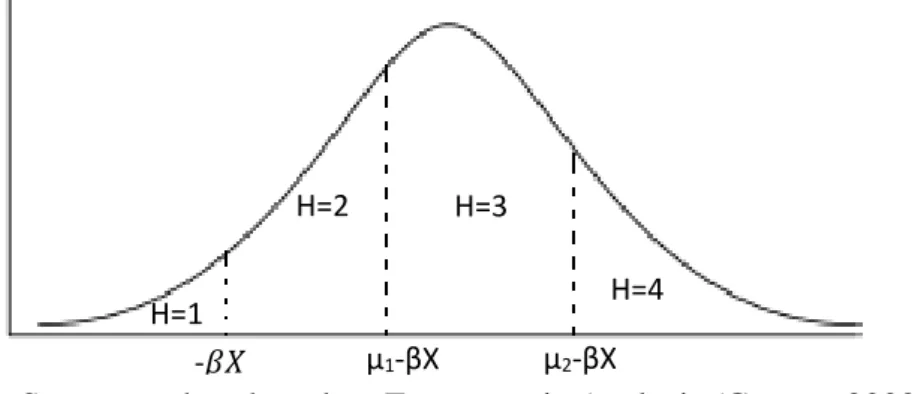
𝐻 = {

1, 𝑖𝑓 𝐻∗ _{≤ 0} 2, 𝑖𝑓 0 < 𝐻∗ _{≤ 𝜇}

1 3, 𝑖𝑓 𝜇1 < 𝐻∗≤ 𝜇2 4, 𝑖𝑓 𝜇2 ≤ 𝐻∗

In this model we assume that εi is normally distributed and when normalizing for

N(0,1) we have the following probabilities, where Φ is the cumulative distribution

function:

Prob (H=1) =Φ (-𝛽𝑋)

Prob (H=2) =Φ (𝜇₁-𝛽𝑋) - Φ (-𝛽𝑋)

Prob (H=3) =Φ (𝜇₂-𝛽𝑋) - Φ (𝜇₁-𝛽𝑋)

Prob (H=4) = 1 - Φ (𝜇₂-𝛽𝑋)

(12)

Figure 3: Normal distribution of function H (happiness)

Source: author, based on Econometric Analysis (Greene, 2003)

The software employed to conduct this work was Stata and all regressions were

carried out using the oprobit function. When using this model it is necessary to calculate

the marginal effect, and the direction and statistical significance must be analyzed. The probability of each of the answers Prob (H=1, 2, 3 or 4) is also computed. All results obtained can be found in the following section.

4. Results

In order for the results to be comparable between countries and years, the same regression was estimated for all countries and waves, except when data was not available

and could not be proxied. The independent variables employed reflect civil status4_{, genre}5_,

health condition6, parenting7, age8, national pride9, education10, employment status11,

4_{Variable with 6 categories in the WVS that was group into 4: single (base), married, divorced and}

widowed

5_{Genre variable: man (base) and woman}

6_{Variable with 4 categories: poor health (base), fair health, good health and very good health} 7_{Variable grouped into 2 categories: no kids (base) and with kids}

8_{Variable grouped into 5 categories: Less than 24 years old (base), between 25 and 34 years old, between}

35 and 44 years old, between 45 and 54 years old and more than 55 years old

9_{Variable with 4 categories: not at all proud (base), not very proud, proud and very proud}

10_{This variable changes among waves. Grouped by no formal education (base), elementary school,}

secondary school and higher education

11_{Variable with 5 categories: unemployed, employed, student, housewife and retired}

H=1

H=2 H=3

H=4

(13)

race12_{, and membership of social organization}13_{. For religion}14_{, a variable to determine} frequency of attending cults was empl oyed, in other words, the level of participation in that religion and not the religious belief itself was considered. As previously mentioned, due to measuring issues and difficulties comparing income, the subjective variable for

social class15 was used instead. Below, tables 2, 3, 4 and 5 show the regression results

obtained. For additional details, the calculated marginal effects for the last wave can be found for all countries in appendix 1.

From the results obtained from tables 2, 3, 4 and 5 we confirm that the determinants for happiness suffer modifications over the years, even for the same country. When we analyze the variable for gender, it is possible to see that it is significant for Brazil and Mexico (wave 2) and Chile (wave 5), for Chile and Mexico the variable is positively associated with happiness, i.e., women are more likely to be happier than men. This result supports Graham and Chattopadhyay's (2012) study, which shows that globally women are happier than men.

When we analyze civil status for the four countries that are the focus of this dissertation we can draw the same conclusions as in Stack and Eshleman (1998), that married people are happier than single, in Brazil and Chile. In the three waves studied the coefficients are positive and statistically significant. Divorced and widowed people tend to be less happy than singles. For the health variables it is possible to once again support studies such as in Graham (2008), for all countries and waves, in that healthier people are happier than those that are not so healthy.

12_{Race variable grouped into 3 categories: white Caucasian (base), black and others races. All black}

variations were grouped in just black. This variable was not available for Argentina on waves 2 and 3

13_{The construction of this variable took into consideration if the person was an active member in one of}

the 10 organizations present in the WVS

(14)

Age and education are two variables that when statistically significant do not have the same effect as presented in Blanchflower and Oswald (2004) and Noval and Garvi

(2012), respectively. For Blanchflower and Oswald (2004) “Age x Happiness” is an U

-shaped curve (with the minimum point at around 50 years old). In Brazil we have found that although younger people are happier, the subsequent age groups do not decline in happiness (see Appendix 1), having in this country the minimum point between 25 and 34 years old. The variable education is negative for Chile and positive for Mexico, in both cases statistically significant, but even when it takes the expected sign (positive) that Noval and Garvi (2012) found, the marginal effect for higher education is inferior than the marginal effect for elementary and secondary school (see appendix 1), different from what was exposed by Noval and Garvi (2012) .

The social class variable although not always significant supports Easterlin (1974). It confirms that wealthier people are happier than those in lower classes. Some scenarios suffer a slight reversion in wave 5 (Argentina).

For the variable "active member of a social organization", it is possible to detect its relevance for Mexico in wave 3 and wave 5, with negative and positive coefficients, respectively. A possible interpretation for this variation was the political scenario in Mexico during 1996 (wave 3), where several conflicts took place and social organizations were involved with manifestations, possibly influencing the coefficient.

(15)

we have observed that national pride, in accordance with Reeskens and Wright (2011) and being religious, as shown by Lim and Putnam (2010) are always positively associated to happiness.

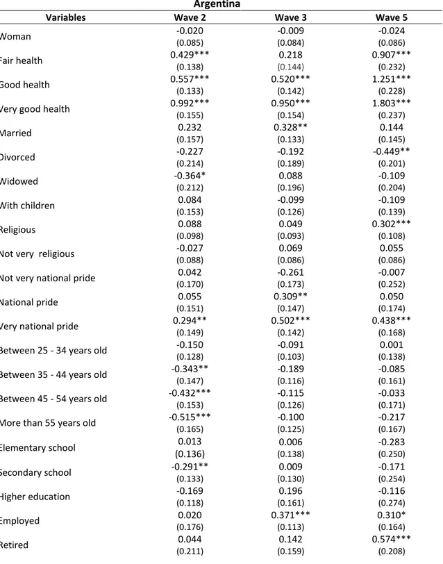
Table 2: Regression Results – Argentina all 3 waves

Argentina

Variables Wave 2 Wave 3 Wave 5

Woman -0.020

(0.085)

-0.009

(0.084)

-0.024

(0.086)

Fair health 0.429***

(0.138)

0.218 (0.144)

0.907***

(0.232)

Good health 0.557***

(0.133)

0.520***

(0.142)

1.251***

(0.228)

Very good health 0.992***

(0.155)

0.950***

(0.154)

1.803***

(0.237)

Married 0.232

(0.157)

0.328**

(0.133)

0.144

(0.145)

Divorced -0.227

(0.214)

-0.192

(0.189)

-0.449**

(0.201)

Widowed -0.364*

(0.212)

0.088

(0.196)

-0.109

(0.204)

With children 0.084

(0.153)

-0.099

(0.126)

-0.109

(0.139)

Religious 0.088

(0.098)

0.049

(0.093)

0.302***

(0.108)

Not very religious -0.027

(0.088)

0.069

(0.086)

0.055

(0.086)

Not very national pride 0.042

(0.170)

-0.261

(0.173)

-0.007

(0.252)

National pride 0.055

(0.151)

0.309**

(0.147)

0.050

(0.174)

Very national pride 0.294**

(0.149)

0.502***

(0.142)

0.438***

(0.168)

Between 25 - 34 years old -0.150

(0.128)

-0.091

(0.103)

0.001

(0.138)

Between 35 - 44 years old -0.343**

(0.147)

-0.189

(0.116)

-0.085

(0.161)

Between 45 - 54 years old -0.432***

(0.153)

-0.115

(0.126)

-0.033

(0.171)

More than 55 years old -0.515***

(0.165)

-0.100

(0.125)

-0.217

(0.167)

Elementary school 0.013

(0.136)

0.006

(0.138)

-0.283

(0.250)

Secondary school -0.291**

(0.133)

0.009

(0.130)

-0.171

(0.254)

Higher education -0.169

(0.118)

0.196

(0.161)

-0.116

(0.274)

Employed 0.020

(0.176)

0.371***

(0.113)

0.310*

(0.164)

Retired 0.044

(0.211)

0.142

(0.159)

0.574***

(16)

Argentina

Housewife 0.024

(0.194)

0.142***

(0.159)

0.344*

(0.193)

Student 0.010

(0.253)

0.275

(0.174)

0.535**

(0.221)

Class AB (upper) 0.179

(0.150)

-0.077

(0.795)

0.563***

(0.154)

Class C (middle) 0.322***

(0.124)

0.175

(0.118)

0.309*

(0.120)

Class D (lower-middle) 0.188

(0.124)

0.020

(0.078)

0.386***

(0.113)

Black - - -0.712***

(0.236)

Other races - - -0.049

(0.123)

Part of social organization -0.001

(0.084)

0.049

(0.078)

0.088

(0.118)

# Observations 986 1068 992

R2 0.059 0.074 0.116

Cut 1 -1.248 -1.006 -0.392

Cut 2 -0.135 0.224 0.850

Cut 3 1.165 1.849 2.684

Notes:

1 –*** significant at 1% ** significant at 5% * significant at 10%

2 – In parenthesis: robust standard error

Table 3: Regression Results – Brazil all 3 waves

Brazil

Woman -0.113*

(0.064)

-0.126

(0.080)

0.041

(0.066)

(0.183)

1.047***

(0.279)

0.322

(0.242)

(0.182)

1.389***

(0.280)

0.678***

(0.243)

(0.190)

1.871***

(0.290)

1.337***

(0.252)

Married 0.369***

(0.107)

0.496***

(0.121)

0.229**

(0.100)

Divorced 0.102

(0.143)

0.145

(0.179)

0.104

(0.131)

Widowed 0.057

(0.163)

0.020

(0.213)

0.095

(0.168)

With children -0.116

(0.104)

-0.272**

(0.122)

-0.004

(0.097)

Religious 0.208***

(0.069)

0.095

(0.110)

0.146**

(0.073)

Not very religious -0.044

(0.064)

-0.216**

(0.100)

0.120

(0.083)

Not very national pride -0.036

(0.143)

-0.368

(0.277)

-0.421***

(0.147)

National pride 0.236**

(0.118)

0.157

(0.274)

-0.140

(17)

Brazil

Very national pride 0.371***

(0.114)

0.120

(0.266)

0.171

(0.129)

Between 25 - 34 years old 0.056

(0.090)

-0.077

(0.103)

-0.367***

(0.110)

(0.087)

-0.034

(0.118)

-0.343***

(0.117)

(0.106)

-0.072

(0.130)

-0.281**

(0.128)

More than 55 years old 0.246**

(0.117)

-0.063

(0.156)

-0.233

(0.144)

Elementary school -0.136

(0.156)

-0.129

(0.135)

0.022

(0.258)

Secondary school -0.131

(0.158)

-0.090

(0.122)

-0.048

(0.261)

(0.177)

-0.128

(0.145)

0.052

(0.265)

Employed 0.101

(0.095)

0.126

(0.111)

0.180**

(0.085)

Retired 0.295**

(0.145)

0.232

(0.162)

0.208 (0.137)

Housewife 0.078

(0.124)

0.211

(0.142)

0.012 (0.128)

Student 0.248

(0.171)

0.006

(0.181)

0.108 (0.157)

Class AB (upper) 0.247**

(0.121)

1.057***

(0.299)

0.188 (0.199)

Class C (middle) 0.077

(0.079)

0.432***

(0.131)

0.237***

(0.084)

Class D (lower-middle) 0.016

(0.065)

0.288***

(0.076)

0.097

(0.081)

Black -0.008

(0.074)

-0.142*

(0.085)

0.051

(0.065)

Other races 0.039

(0.211)

-0.292

(0.185)

0.186

(0.186)

(0.058)

0.114

(0.075)

0.051

(0.145)

R2 0.056 0.104 0.086

Cut 1 -0.824 -0.722 -1.702

Cut 2 0.547 0.552 -0.395

Cut 3 2.184 2.517 1.517

Notes:

Table 4: Regression Results – Chile all 3 waves

Chile

Woman 0.040

(0.072)

-0.170*

(0.092)

0.150*

(0.087)

(0.143)

0.484***

(0.186)

0.516***

(18)

Chile

(0.145)

0.721***

(0.186)

0.765***

(0.187)

(0.164)

1.155***

(0.209)

1.468***

(0.209)

Married 0.348***

(0.112)

0.254**

(0.107)

0.232*

(0.129)

Divorced 0.020

(0.165)

-0.290

(0.190)

-0.265

(0.165)

Widowed 0.009

(0.175)

-0.237

(0.191)

-0.242

(0.229)

(0.106)

0.436

(0.628)

0.054

(0.134)

Religious 0.244***

(0.074)

0.384***

(0.100)

0.160

(0.103)

Not very religious 0.110

(0.071)

0.056

(0.089)

-0.070

(0.084)

Not very national pride 0.082

(0.213)

0.238

(0.325)

-0.534

(0.326)

(0.201)

0.461

(0.313)

-0.395

(0.281)

Very national pride 0.382*

(0.201)

0.743** (0.314)

-0.190

(0.280)

(0.091)

-0.055

(0.120)

-0.019

(0.154)

(0.106)

-0.079

(0.137)

-0.146

(0.173)

Between 45 - 54 years old -0.213*

(0.114)

-0.179

(0.140)

-0.253

(0.186)

More than 55 years old -0.204*

(0.119)

-0.106

(0.151)

-0.158

(0.190)

Elementary school 0.021

(0.139)

-0.321*

(0.194)

-0.636**

(0.312)

Secondary school -0.001

(0.122)

-0.352**

(0.157)

-0.576*

(0.316)

(0.113)

-0.383**

(0.175)

-0.692**

(0.336)

Employed 0.129

(0.140)

0.044

(0.178)

0.389**

(0.161)

Retired -0.064

(0.181)

0.012

(0.238)

0.372*

(0.215)

Housewife 0.229

(0.156)

0.137

(0.205)

0.322*

(0.181)

Student 0.227

(0.165)

0.124

(0.220)

0.541**

(0.212)

Class AB (upper) 0.435***

(0.118)

0.628

(0.727)

0.637***

(0.152)

(0.084)

0.344***

(0.117)

0.328***

(0.117)

Class D (lower-middle) 0.260***

(0.081)

0.223***

(0.087)

0.171

(0.122)

Black -0.469

(0.360) -

-0.829**

(0.418)

Other races -0.103

(0.154)

-0.021

(0.123)

0.213

(19)

Chile

(0.060)

0.090

(0.078)

0.151*

(0.078)

R2 0.056 0.087 0.105

Cut 1 -0.555 -1.087 -1.755

Cut 2 0.923 0.761 -0.291

Cut 3 2.033 2.378 1.290

Notes:

Table 5: Regression Results – Mexico all 3 waves

Mexico

Woman 0.163**

(0.068)

0.038

(0.056)

0.023

(0.083)

Fair health 0.302*

(0.164)

0.650***

(0.097)

0.591***

(0.173)

(0.161)

1.238***

(0.097)

0.991***

(0.176)

(0.169)

1.831***

(0.111)

1.654***

(0.190)

Married 0.141

(0.117)

0.070

(0.094)

0.069

(0.117)

Divorced -0.317*

(0.176)

-0.083

(0.124)

-0.404***

(0.157)

Widowed -0.112

(0.170)

-0.181

(0.156)

-0.259

(0.194)

(0.112)

-0.180**

(0.090)

0.094

(0.114)

Religious 0.060

(0.075)

0.010 (0.061)

0.133

(0.088)

Not very religious 0.069

(0.077)

-0.047 (0.064)

0.068

(0.088)

Not very national pride -0.205

(0.194)

-0.059 (0.137)

0.178

(0.388)

(0.174)

0.115 (0.113)

0.200

(0.363)

Very national pride 0.163

(0.173)

0.559***

(0.109)

0.502

(0.355)

(0.086)

-0.069

(0.070)

0.139

(0.105)

(0.102)

0.013

(0.082)

0.045

(0.118)

0.037

(0.092)

0.057

(0.123)

More than 55 years old -0.166

(0.141)

0.255**

(0.113)

-0.002

(0.136)

Elementary school -0.048

(0.138)

0.034

(0.096)

0.426***

(20)

Mexico

Secondary school 0.026

(0.104)

0.001

(0.086)

0.481***

(0.148)

(0.075)

0.085

(0.101)

0.340**

(0.159)

Employed -0.113

(0.134)

0.183**

(0.092)

0.205*

(0.121)

Retired -0.187

(0.220)

-0.113

(0.160)

0.335

(0.217)

Housewife -0.179

(0.157)

0.043

(0.106)

0.196

(0.142)

Student -0.191

(0.156)

0.113

(0.116)

0.217

(0.190)

Class AB (upper) 0.456***

(0.101)

0.576***

(0.147)

0.368**

(0.155)

(0.083)

0.235***

(0.071)

0.192

(0.144)

Class D (lower-middle) 0.239***

(0.078)

0.077

(0.055)

0.113

(0.147)

Black -0.064

(0.073)

-0.988***

(0.280)

0.014

(0.079)

Other races -0.159

(0.146)

0.070

(0.065)

0.109

(0.260)

Part of social organization 0.080 (0.061)

-0.142***

(0.050)

0.120*

(0.120)

R2 0.049 0.134 0.102

Cut 1 -1.443 -0.787 -0.326

Cut 2 0.168 0.996 0.995

Cut 3 1.419 2.237 2.288

Notes:

1 – *** significant at 1%, ** significant at 5%, * significant at 10%

(21)

Chart 2: Happiness x Health - Wave 5 for all countries

Source: Author

(22)

Chart 3: Happiness x Social Class- Wave 5 for all countries

Source: Author

5. Conclusion

This dissertation has the intention to examine the socioeconomic determinants that directly affect the self-perception of happiness. We observed for all four countries studied that having a good health is the most important statement for an individual to be self-declared happy. For Argentinians being happy is also related to religion, social class and formal occupation; for Brazilians being happy is associated to being married and young; for Chileans being female increases happiness while being of the black race decreases the happiness perception and for Mexicans being a member of a social organization and having formal education raises the happiness probability.

(23)

overall population well-being. In countries such as the United States and England, happiness and well-being studies are frequently used as a government source.

The results we observed showed that happiness determinants change across countries and years, but we also observed that some of them have always significance to increase or decrease happiness, so that these ones are the ones that should be the focus of any public policy for well-being.

This dissertation confirmed some existing results in the literature regarding genre, social class, religious and health, however, it does not support existing results regarding education and age. It is important to note that when specifically discussing Latin America these results are new and should contribute to the understanding of the determinants of happiness for people in developing countries.

(24)

6. Appendix

Marginal Effects - Wave 5 dy/dx - “Very Happy” probability

Variables Argentina Brasil Chile México

Woman -0.008 0.015 0.052* 0.009

Fair health 0.338*** 0.119 0.188*** 0.219***

Good health 0.418*** 0.242*** 0.264*** 0.362***

Very good health 0.619*** 0.491*** 0.536*** 0.487***

Married 0.049 0.082** 0.080* 0.027

Divorced -0.136*** 0.038 -0.087 -0.160***

Widowed -0.036 0.035 -0.079 -0.102

With children -0.017 0.001 0.019 0.037

Religious 0.108*** 0.052** 0.057 0.051

Not very religious 0.019 0.043 -0.023 0.026

Not very national pride -0.002 0.138*** -0.159 0.067

National pride 0.017 0.050 -0.132 0.076

Very national pride 0.146*** 0.062 -0.067 0.197

Between 25 - 34 years old 0.001 -0.125*** -0.007 0.053

Between 35 - 44 years old -0.029 -0.117*** -0.050 0.017

Between 45 - 54 years old -0.011 -0.096** -0.084 0.022

More than 55 years old -0.072 -0.081 -0.054 -0.001

Elementary School -0.094 0.008 -0.197** 0.160***

Secondary school -0.059 0.017 -0.204* 0.183***

Higher Education -0.038 0.019 -0.208** 0.128**

Employed 0.105** 0.065** 0.135** 0.079*

Retired 0.213*** 0.077 0.138* 0.123

Housewife 0.124* 0.004 0.117* 0.075

Student 0.200** 0.040 0.205** 0.082

Class AB (upper) 0.210*** 0.070 0.240*** 0.137**

Class C (middle) 0.109*** 0.086*** 0.115*** 0.074

Class D (lower-middle) 0.133*** 0.035 0.061 0.043

Black -0.187*** 0.018 -0.214*** 0.005

Other races -0.016 0.069 0.077 0.042**

Part of social organization 0.029 0.018 0.053* 0.047

(25)

7. Bibliography

Aristotle. 2000. Nicomachean Ethics. Cambridge, UK: Cambridge University Press.

Bentham, J. (1789) . An Introduction to the Principles of Morals and Legislation.

London, T.Payne.

Bergheim, Stefan. 2006. “Measures of well-being: There is more to it than GDP”.

Deutsche Bank Research [Available at

http://www.dbresearch.com/PROD/DBR_INTERNET_EN-PROD/PROD0000000000202587.PDF acessed in 15 August 2014]

Blanchflower, D. G. and A. J. Oswald (2004). “Well-being over time in Britain and the

USA”. Journal of public economics, 88(7), 1359-1386.

Cheah, Yong Kang and Chor Foon Tang . 2013. “The socio-demographic determinants

of self-rated happiness: The case of Penang, Malaysia”. Hitotsubashi Journal of

Economics

Corbi, R. B. and Naércio Menezes-Flho. 2006. “Os determinantes empíricos da

felicidade no Brasil”. Magazine of Economia Política, v. 26, n. 4.

Easterlin, Richard A. (1974). “Does economic growth improve the human Lot? Some empirical evidence.”

Graham, Carol. (2008). “Happiness and health: Lessons—and questions—for public policy”. Health affairs, 27(1), 72-87.

Graham, Carol, and Soumya Chattoadhyay. 2012. “Gender and Well-Being around the

World: Some Insights from the Economics of Happiness”. The Brookings Institution,

University of Chicago, Chicago, USA.

Greene, W., 2003, Econometric Analysis. Fifth Ed., Macmillan Publishing Company,

New York.

Helliwell, John, Richard Layard and Jeffrey Sachs. 2012. “World happiness report.”

The Earth Institute, Columbia University, New York, USA. [Available at

http://eprints.lse.ac.uk/47487/1/World%20happiness%20report%28lsero%29.pdf

accessed on 15 August 2014]

Helliwell, John, Richard Layard and Jeffrey Sachs. 2013. “World happiness report.” The Earth Institute, Columbia University, New York, USA. [Available at

http://unsdsn.org/wp-content/uploads/2014/02/WorldHappinessReport2013_online.pdf

accessed on 15 August 2014]

Lim, Chaeyoon, and Robert D. Putnam. 2010. "Religion, social networks, and life

satisfaction". American Sociological Review 75, no. 6 (2010): 914-933.

(26)

Moro, Mirko and Finbarr Brereton and Susana Ferreira, and J. Peter Clinch. 2008.

“Ranking quality of life using subjective well-being data”. Ecological Economics,

Volume 65, Issue 3, 15 April 2008, Pages 448–460

Myrskylä, Mikko, and Rachel Margolis.2014. "Happiness: Before and after the kids". Noval, Borja López, and Marta Guijarro Garvi. "Empirical Relationship between Education and Happiness. Evidence from SHARE".

Pukeliene, Violeta and Justinas Kisieliauskas. 2013. “The influence of income on

subjective well-being”. Taikomoji Ekonomika

Reeskens, Tim, and Matthew Wright.2011. "Subjective Well-Being and National Satisfaction Taking Seriously the “Proud of What?” Question." Psychological science 22, no. 11 (2011): 1460-1462.

Seligman, M. E. P. (2002). “Authentic happiness". New York: Free Press

Stack, Steven and J Ross Eshleman. 1998 . “Marital status and happiness: A 17-nation

study”. Journal of Marriage and the Family; May 1998; 60, 2; Research Library pg.

527

Tetaz, Martin. 2012. “The Economics of Happiness in Argentina”. Palermo Business Review , Nº 7 .

WORLD VALUES SURVEY Wave 2 1990-1994 OFFICIAL AGGREGATE v.20140429. World Values Survey Association (www.worldvaluessurvey.org). Aggregate File Producer: Asep/JDS, Madrid SPAIN.

WORLD VALUES SURVEY Wave 3 1995-1998 OFFICIAL AGGREGATE v.20140921. World Values Survey Association (www.worldvaluessurvey.org). Aggregate File Producer: Asep/JDS, Madrid SPAIN.