Nonlocal continuum mechanics formulation for axial, flexural,
shear and contraction coupled wave propagation in single walled
carbon nanotubes
Abstract
This paper presents the effect of nonlocal scaling parameter on the coupled i.e., axial, flexural, shear and contraction, wave propagation in single-walled carbon nanotubes (SWC-NTs). The axial and transverse motion of SWCNT is mod-eled based on first order shear deformation theory (FSDT) and thickness contraction. The governing equations are de-rived based on nonlocal constitutive relations and the wave dispersion analysis is also carried out. The studies shows that the nonlocal scale parameter introduces certain band gap region in all wave modes where no wave propagation occurs. This is manifested in the wavenumber plots as the region where the wavenumber tends to infinite or wave speed tends to zero. The frequency at which this phenomenon occurs is called the escape frequency. Explicit expressions are derived for cut-off and escape frequencies of all waves in SWCNT. It is also shown that the cut-off frequencies of shear and contraction mode are independent of the nonlocal scale parameter. The results provided in this article are new and are useful guidance for the study and design of the next generation of nanodevices that make use of the coupled wave propagation properties of single-walled carbon nanotubes. Keywords
Carbon Nanotube, Wavenumber, Group Velocity, Nonlocal Elasticity, Escape Frequency, Dispersion.
S. Narendara,∗
and S. Gopalakrishnanb
a
Defence Research and Development Labora-tory, Kanchanbagh, Hyderabad-500 058, India. Tel.: +91 88976 25977 / +91 9949391823. b
Computational Wave Mechanics Laboratory, Department of Aerospace Engineering, Indian Institute of Science, Bangalore-560 058, India.
Received 17 Apr 2012; In revised form 30 Apr 2012
∗Author email: [email protected]
1 INTRODUCTION
shown that the Young modulus of multi-walled carbon nanotubes is approximately 1.28 TPa [21], which is about two orders of magnitude larger than that of steel.
Carbon nanotubes can have interesting waveguide properties at very high frequencies in the order of Tera-Hertz (THz). At such high frequencies, continuum model based finite element type methods cannot be adopted due to their limitation of the element size with respect to the wavelength, which is very small at such frequencies. Lattice dynamics for direct observation of phonons [1, 2, 10] and spectral finite element type method are more efficient and consistent to analyze such problem [11]. The nanostructures length scales are often sufficiently small, and hence for the applicability of classical continuum models, we need to consider the small length scales such as lattice spacing between individual atoms, grain size, etc. Although solution through Molecular Dynamics (MD) simulation is a possibility for such problems, its large computational cost prohibits its use for a general analysis. The conventional continuum models cannot handle scale effects. Hence the best alternative is to use those methods which provides the simplicity of continuum models and at the same time incorporate the effects of scale in such chosen continuum models [12, 20, 23, 25, 29].
An important class of modified continuum models are those based on the concept of nonlocal elasticity. These models allow the integration of small-size effects into classical continuum models. The theory of nonlocal elasticity introduced by Eringen in the 1970s was originally used to study screw dislocation and surface waves in solids [4–6]. Unlike classical continuum models, the nonlocal elasticity theory assumes that the stress at a reference point in a body depends not only on the strains at that point, but also on strains at all other points of the body. This nonlocal effect becomes significant when the features of a body such as the size of an imperfection or the length of a traveling wave become comparable to the intrinsic length scales of the system such as the inter-atomic distance or the particle spacing of a lattice structure.
In the present paper, first order shear deformation theory (FSDT) is used, that includes the contribution of stiffness and inertial coupling for studying the characteristic wave propagation in carbon nanotubes. Appearance of higher order Lamb wave modes above certain cut-off frequencies have been studied for metallic beams by Mindlin and Harrmann [22], Doyle [3] and Gopalakrishnan [7] and for laminated composite plates by Karim et al. [11]. In the present paper, contribution of a contractional mode along with shear mode is studied for SWCNTs. Expression of cut-off frequencies and escape frequencies in shear mode and contractional mode are also derived.
The paper is organized as follows. In section 2, Erigen’s nonlocal elasticity theory is explained and the coupled wave propagation equations for SWCNT are derived including the nonlocal scale effects. The effect of nonlocal scaling parameter(e0a) on the wave propagation
in SWCNTs and also the variation of the escape and cut-off frequencies with nanotube radius and e0a is studied in detail. In section 3, some numerical results are presented on the wave
dispersion in SWCNTs. The expressions for the wavenumbers and wave speeds (i.e., phase and group speeds) are also derived. The paper ends with some important observations and conclusions.
2 MATHEMATICAL FORMULATION 2.1 Theory of Nonlocal Elasticity
The length scales associated with nano structures like CNTs are such that to apply any classical continuum techniques, we need to consider the small length scales such as lattice spacing between individual atoms, grain size, etc. This makes the consistent classical continuum model formulation very challenging. The Eringen’s nonlocal elasticity theory [4, 6] is useful tool in treating the phenomena whose origins lie in the regimes smaller than the classical continuum models.
This theory assumes that the stress state at a reference pointx=(x1, x2, x3)in the body is
regarded to be dependent not only on the strain state atxbut also on the strain states at all other points x′
of the body. This is in accordance with atomic theory of lattice dynamics and experimental observations on phonon dispersion. The most general form of the constitutive relation in the nonlocal elasticity type representation involves an integral over the entire region of interest. The integral contains a nonlocal kernel function, which describes the relative influences of the strains at various locations on the stress at a given location. The constitutive equations of linear, homogeneous, isotropic, non-local elastic solid with zero body forces are given by
σkl,k+ρ(fl−u¨l)=0 (1)
σkl(x)=∫
V α(∣x
−x′
∣, ξ)σklc (x′
)dV(x′
) (2)
σckl(x′
)=λerr(x ′
)δkl+2µekl(x ′
ekl(x ′
)= 1
2(
∂uk(x
′
)
∂x′
l
+∂ul(x
′
)
∂x′
k
) (4)
Equation (1) is the equilibrium equation, where σkl, ρ, fl and ul are the stress tensor, mass density, body force density and displacement vector at a reference pointx in the body, respectively, at time t. Equation (3) is the classical constitutive relation where σckl(x′
) is the classical stress tensor at any point x′
in the body, which is related to the linear strain tensor ekl(x
′
) at the same point through the lame constants λ and µ. Equation (4) is the classical strain-displacement relationship. The only difference between equations (1)-(4) and the corresponding equations of classical elasticity is the introduction of equation (2), which relates the global (or nonlocal) stress tensorσkl to the classical stress tensorσckl(x′)using the modulus of nonlocalness. The modulus of nonlocalness or the nonlocal modulusα(∣x−x′
∣, ξ) is the kernel of the integral equation (2) and contains parameters which correspond to the nonlocalness [16]. A dimensional analysis of equation (2) clearly shows that the nonlocal modulus has dimensions of (length)−3
and so it depends on a characteristic length ratioa/ℓ whereais an internal characteristic length (lattice parameter, size of grain, granular distance) and ℓ is an external characteristic length of the system (wavelength, crack length, size or dimensions of sample) [4]. Therefore the nonlocal modulus can be written in the following form:
α=α(∣x−x′
∣, ξ), ξ= e0a
ℓ (5)
wheree0is a constant appropriate to the material and has to be determined for each material
independently [4].
Making certain assumptions [4], the integro-partial differential equations of nonlocal elas-ticity can be simplified to partial differential equations. For example, equation (2) takes the following simple form:
(1−ξ2ℓ2∇2)σkl(x)=σklc(x)=Cklmnεmn(x) (6) where Cijkl is the elastic modulus tensor of classical isotropic elasticity and εij is the strain tensor. where ∇2 denotes the second order spatial gradient applied on the stress tensor σkl,k and ξ =e0a/ℓ. The validity of equation (6) has been justified by comparing the expressions
for frequency of waves from the nonlocal model above with those of the Born-Karman model of lattice dynamics [4]. Eringen reports a maximum difference of 6% and a perfect match for nonlocal constant value ofe0=0.39 [4]. Sudak [18] proposed thate0=112.7 for the critical axial
strain of a double walled carbon nanotube. To the best of authors knowledge, no experiments have been conducted on CNT to determine the value ofe0. Wang and Hu [19] proposed that
e0 = 1/
√
12 and used this value in the non-local beam model. Zhang et al. [29] estimated that e0≈0.82 by matching the theoretical buckling strain obtained by the nonlocal thin shell
SWCNT wave propagation at frequencies grater than 10 THz. e0, which is a nonlocal scaling
parameter, which has been assumed as a constant appropriate to each material in published literature.
2.2 Derivation of the Nonlocal Governing Partial Differential Equations
The displacement field for axial and transverse motion based on first order shear deformation theory (FSDT) and thickness contraction is given by
u(x, y, z, t)=u0(x, t)−zϕ(x, t) (7)
w(x, y, z, t)=w0(x, t)+zψ(x, t) (8)
whereuandware the axial and transverse displacements, respectively, at a material point. u0
is the beam axial displacement along the reference plane,w0
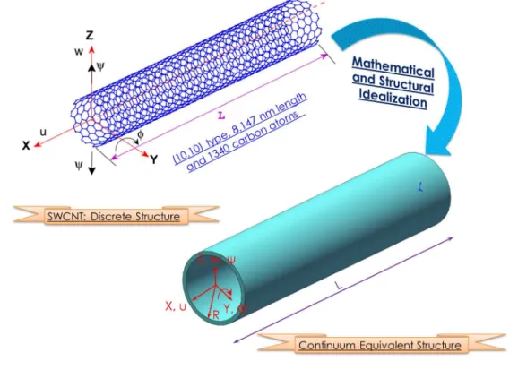
is the transverse displacement on the reference plane,ϕ is the curvature- independent rotation of the beam cross-section about Y-axis and ψ=εzz is the contraction/elongation parallel to Z-axis (shown in Fig. 1).
The strains are obtained as
εxx= ∂u
0
(x, t)
∂x −z
∂ϕ(x, t)
∂x (9)
εzz=ψ(x, t) (10)
εxz=−ϕ(x, t)+
∂w0(
x, t)
∂x +z
∂ψ(x, t)
∂x (11)
Using Hamilton’s principle and Eqs. (1) and (2), the governing wave equations can be obtained as The nonlocal constitutive relation for isotropic materials is given as [16]
⎧⎪⎪⎪ ⎨⎪⎪⎪ ⎩ σxx σzz τxz ⎫⎪⎪⎪ ⎬⎪⎪⎪ ⎭
−(e0a) 2 ∂ 2 ∂x2 ⎧⎪⎪⎪ ⎨⎪⎪⎪ ⎩ σxx σzz τxz ⎫⎪⎪⎪ ⎬⎪⎪⎪ ⎭ = ⎡⎢ ⎢⎢ ⎢⎢ ⎣
C11 νC12 0
νC12 C22 0
0 0 C66
⎤⎥ ⎥⎥ ⎥⎥ ⎦ ⎧⎪⎪⎪ ⎨⎪⎪⎪ ⎩ εxx εzz γxz ⎫⎪⎪⎪ ⎬⎪⎪⎪ ⎭ (12)
where, σxx and σzz are the normal stresses in x and z directions respectively and τxz is the in-plane shear stress. For the case of an isotropic plate, the expressions for Cij in terms of Young’s modulus E and Poisson’s ratio ν are given as C11 = C12 = C22 = E/(1−ν
2
) and
C66=E/(2(1+ν)).
The potential and kinetic energies are given as
ΠE= 1
2∫V (
σxxεxx+σzzεzz+τxzγxz)dV
= 1
2∫ L
0 ∫A(
σxxεxx+σzzεzz+τxzγxz)dxdA
(13)
ΓE= 1
2ρ∫V (˙
u2+w˙2)dV
= 1
2ρ∫ L
0 ∫A([u˙ 0
(x, t)−zϕ˙(x, t)]2+[w˙0(x, t)+zψ˙(x, t)]2)dxdA
(14)
assuming constant cross-sectional area of SWCNT,
ΠE= 1
2A∫ L
0 (
σxxεxx+σzzεzz+τxzγxz)dx (15)
ΓE= 1
2ρA∫ L
0 ([u˙ 0
(x, t)−zϕ˙(x, t)]2+[w˙0(x, t)+zψ˙(x, t)]2)dx (16) Using Hamilton’s principle,
∫tt2 1
δ£Edt=∫
t2
t1
and Eqs. (9 )-(11) and (12), and the fundamental lemma of calculus of variations, the nonlocal governing equations of motion are derived as:
δu0∶I0
∂2
u0
∂t2 −I0(e0a)
2 ∂ 4
u0
∂t2∂x2 −I1
∂2
ϕ
∂t2 +I1(e0a)
2 ∂ 4
ϕ
∂t2∂x2
−C11J0
∂2u0
∂x2 +C11J1
∂2ϕ
∂x2 −C12J0
∂ψ
∂x =0
(18)
δψ∶ I2
∂2ψ
∂t2 −I2(e0a)
2 ∂ 4
ψ
∂t2∂x2+I1
∂2w0
∂t2 +I1(e0a)
2 ∂ 4
w0
∂t2∂x2+C12J0
∂u0
∂x −C12J1
∂ϕ ∂x
+C22J0ψ−C66J1(
∂2w0
∂x2 −
∂ϕ
∂x)C66J2
∂2ψ
∂x2 =0
(19)
δw0∶ I0
∂2w0
∂t2 −I0(e0a)
2 ∂ 4
w0
∂t2∂x2 +I1
∂2ψ
∂t2 −I1(e0a)
2 ∂ 4
ψ
∂t2∂x2
−C66J0(
∂2
w0
∂x2 −
∂ϕ
∂x)−C66J1
∂2
ψ
∂x2 =0
(20)
δϕ∶ I2
∂2
ϕ
∂t2 −I2(e0a)
2 ∂ 4
ϕ
∂t2∂x2−I1
∂2
u0
∂t2 +I1(e0a)
2 ∂ 4
u0
∂t2∂x2 −C66J0(
∂w0
∂x −ϕ)
−C66J1
∂ψ
∂x +C11J1
∂2
u0
∂x2 −C11J2
∂2
ϕ
∂x2 +C11J1
∂ψ
∂x =0
(21)
where
Jp=∫
2π
0 ∫
R+h
R−h
zprdrdθ, (22)
Ip=∫
2π
0 ∫
R+h
R−h
ρzprdrdθ (23)
Here z =rsinθ and p =0,1,2. One can substitute e0a= 0 in the equations (18)-(21), to
recover the local or classical coupled equations for the SWCNTs.
2.3 Wave Dispersion Analysis
2.3.1 Computation of Wavenumbers
Using discrete Fourier transformation (DFT) for the temporal field, the spectral solution for primary displacement field variables can be expressed as
d(x, t)=dˆ(x, ω)e−j(kx−ωt)
where d = {u0 ψ w0 ϕ}T is the generic displacement vector as a function of (x, t) and
ˆ
d = {uˆ0 ψˆ wˆ0 ϕˆ}T represents the the spectral amplitude vector corresponding to generic
displacement vector as a function of(x, ω). dˆ(x, ω)is the frequency domain amplitude vector of the CNTs. k is the wavenumber and ω is the angular frequency of the wave motion and
j=√−1.
Substituting Eqs. (24) in the governing equations of motion of SWCNT (see Eqs. (18)-(21) yields four homogeneous equations in terms of ˆu,ψ,ˆ wˆ and ˆϕas
⎡⎢ ⎢⎢ ⎢⎢ ⎢⎢ ⎣
Q11 Q12 Q13 Q14
Q21 Q22 Q23 Q24
Q31 Q32 Q33 Q34
Q41 Q42 Q43 Q44
⎤⎥ ⎥⎥ ⎥⎥ ⎥⎥ ⎦ ⎧⎪⎪⎪⎪ ⎪⎪ ⎨⎪⎪⎪ ⎪⎪⎪⎩ ˆ u0 ˆ ψ ˆ w0 ˆ ϕ ⎫⎪⎪⎪⎪ ⎪⎪ ⎬⎪⎪⎪ ⎪⎪⎪⎭= ⎧⎪⎪⎪⎪ ⎪⎪ ⎨⎪⎪⎪ ⎪⎪⎪⎩ 0 0 0 0 ⎫⎪⎪⎪⎪ ⎪⎪ ⎬⎪⎪⎪ ⎪⎪⎪⎭ (25)
where[Qab], (a, b=1,2,3,4)are given in appendix A. The wavenumbers and hence the wave speeds (i.e., phase and group speeds) are solved from Eq. (25) by using Polynomial Eigenvalue Problem (PEP) [3, 7, 8, 11, 13, 22]. Equating the determinant of matrix [Qab] to zero (for the non-trivial solution of ˆd will give the characteristic polynomial in terms of wavenumberk of the order 8, solution of which is quite difficult. PEP converts the characteristic polynomial equation into a matrix of size 4×4, whose eigen values form the solution of the equation. After
obtaining the wavenumbers, the wave speeds are extracted. The details of computation of wavenumbers using PEP are as follows.
[S2]k2+[S1]k+[S0]=0 (26)
where S2= ⎡⎢ ⎢⎢ ⎢⎢ ⎢⎢ ⎢⎣
S2(11) 0 0 S
(14) 2
0 S2(22) S
(23)
2 0
0 S2(32) S
(33)
2 0
S2(41) 0 0 S
(44) 2 ⎤⎥ ⎥⎥ ⎥⎥ ⎥⎥ ⎥⎦ (27)
[S1]=
⎡⎢ ⎢⎢ ⎢⎢ ⎢⎢ ⎣
0 −jC12J0 0 0
jC12J0 0 0 −j(C12−C66)J1
0 0 0 jC66J0
0 j(C12−C66)J1 −jC66J0 0
⎤⎥ ⎥⎥ ⎥⎥ ⎥⎥ ⎦ (28)
[S0]=
⎡⎢ ⎢⎢ ⎢⎢ ⎢⎢ ⎣
I0ω2 0 0 −I1ω2
0 −C22J0+I2ω 2
I1ω
2
0
0 I1ω
2
I0ω
2
0
−I1ω 2
0 0 −C66J0+I2ω 2 ⎤⎥ ⎥⎥ ⎥⎥ ⎥⎥ ⎦ (29)
curve and in this figure, the frequency at which the imaginary part of wavenumber becomes real is called as cut-off frequency. The cut-off frequencies of this SWCNTs are obtained by setting k=0 in the dispersion relation (Eq. (26)) i.e., for the present case of PEP one can set Det([S0])=0, for the cut-off frequencies as
ωaxialc =0, ωcf lexural=0 (30)
ωccontraction=
¿ Á Á
ÀC22I0J0
I0I2−I12
, ωcshear =
¿ Á Á
ÀC66I0J0
I0I2−I12
(31)
Fig. 1 shows the spectrum relation plot as a function of nonlocal scale parametere0a. From
the figure, we see that at certain frequencies, the wavenumber is tending to infinity and this frequency value decreases with increase in the scale parameter. Its value can be analytically determined by looking at the wavenumber expression and setting k →∞. This accounts to
setting theDet[S2]=0, which gives
ωeaxial= 1/e0a
√
C66
[2(I0I2−I12)
√
X2−4I1J1X1+4X0−2I0I2J0J2+X1−2I1J1]
1/2 (32)
ωef lexural=
√
C66
e0a [
√
X2−4I1J1X1+4X0−2I0I2J0J2−X1+2I1J1
2(I2
1−I0I2)
]
1/2
(33)
ωsheare = 1/e0a
√
C11
[2(I0I2−I12)
√
X2−4I1J1X1+4X0−2I0I2J0J2+X1−2I1J1]
1/2 (34)
ωecontraction=
√
C11
e0a [
√
X2−4I1J1X1+4X0−2I0I2J0J2−X1+2I1J1
2(I2
1−I0I2)
]
1/2
(35)
where X2=I 2 0J
2 2+I
2 2J
2
0; X1=I0J2+I2J0; X0=I0I2J 2 1+I
2
1J0J2. Here ωe is called escape
fre-quency or sometimes asymptotic frefre-quency. Differentiating the Eq. (26 ) with respect to the wave frequency (ω), one can obtain the group speeds as
2ω((e0a) 2
k2+1) [H]Cg+2k[S2]+[S1]=0 (36)
Here H= ⎡⎢ ⎢⎢ ⎢⎢ ⎢⎢ ⎣
I0 0 0 −I1
0 I2 I1 0
0 I1 I0 0
−I1 0 0 I2
⎤⎥ ⎥⎥ ⎥⎥ ⎥⎥ ⎦ (37)
whereCg =(∂ω/∂kω)is the group speed of a wave in SWCNT and the matrices[S2], and[S1]
solve it for group speeds of respective modes (i.e., for axial, flexural, shear and contraction), which is again a function of nonlocal scale parameter.
The phase speed is calculated from the definition as
Cp=Re(
ω
kω) (38)
The detail effect of the nonlocality on wave speeds of single walled carbon nanotubes will be discussed in the next section.
3 RESULTS AND DISCUSSION
In this section, numerical experiments are presented to analyze the wave properties of SWC-NTs. First, the wavenumber, phase and group speeds are obtained for SWCNT from local and nonlocal elastic theories. Following Wang [20], the nonlocal parametere0a should be less
than 2.0 nm, so that here in the simulation procedure we choosee0a=0nm and 0.5nm. The
spectrum and dispersion curves are plotted for e0a=0nm and 0.5nm.
Fig. (2) shows the real and imaginary parts of the wavenumber of SWCNT obtained from both local and nonlocal models. These wavenumbers are obtained by solving the PEP given in Eq. (26 ). Thick lines represent the real part and the thin lines show the imaginary part of the wavenumbers. From Fig. (2), it can be seen that there are four modes of wave propagation, namely, axial, flexural, shear and contractional. For local/classical elasticity (e0a = 0), the
wavenumbers for the axial mode has a linear variation with the frequency which is in the tera hertz (THz) range. The linear variation of the wavenumbers denote that the waves will propagate non-dispersively, i.e., the waves do not change their shapes as they propagate. On the other hand, the flexural wavenumbers have a non-linear variation with the frequency at low frequencies, which indicates that the waves are dispersive in nature. At high frequencies, the flexural waves show a linear variation with frequency. However, the wavenumbers of this flexural wave mode have a substantial real part starting from the zero frequency. This implies that the mode starts propagating at any excitation frequency and does not have a cut-off frequency. The shear and contractional wave modes, however, have certain frequency band within which the corresponding wavenumbers are purely imaginary. Thus, these modes does not propagate at frequencies lying within this band. Both the shear and contraction wavenumbers have a substantial imaginary part along with the real part, thus these waves attenuate as they propagate. In the present study for a 3.5 nm radius SWCNT, we have shear cut-off frequency at 0.8545 T Hz and contraction cut-off frequency at 1.404 T Hz. The values of the cut-off frequency are calculated from Eq. (31 ). It can be observed from Eq. (31 ) that these frequencies are independent of the nonlocal scaling parameter, and hence same frequencies are obtained from both local and nonlocal theories.
For e0a=0, which is the case of local theory of elasticity solution, wavenumbers increase
0 2 4 6 8 10 0
1 2 3 4 5 6 7 8 9 10
Frequency [THz]
Wavenumber [1/nm]
0 1 2
0 0.5 1
Axial Flexural
Contraction Shear
Nonlocal modes
Local modes
Figure 2 A Comparison of the wavenumber dispersion in SWCNT obtained from local and nonlocal elasticity theories.
effects (for present analysise0a=0.5nm), the wave behavior is altered drastically. All the wave
modes escapes to infinity (as shown in Fig. 2), at a particular frequency called the ”escape frequency”, beyond this frequency there is no wave propagation i.e, the wavenumber before escape frequency are real and after that are purely imaginary. Thus, scale parameter introduces the escape frequency where the wavenumber k tends to infinite and the corresponding wave speeds (i.e, phase and group speeds) tends to zero as shown in Figs. (3) and (4).
0 1 2 3 4 5 6 7 8
0 5 10 15 20 25 30 35 40 45 50
Frequency [THz]
Phase Velocity [Km/s]
Contraction mode
Axial mode
Flexural mode
Shear mode
Local
Nonlocal
0 1 2 3 4 5 6 7 8 0
5 10 15 20 25
Frequency [THz]
Group Velocity [Km/s]
Axial mode
Shear mode
Contraction mode
Flexural mode Local
Nonlocal
Figure 4 A Comparison of the wavenumber dispersion in SWCNT obtained from local and nonlocal elasticity theories.
0 1 2 3 4 5 6 7 8
0 5 10 15 20 25 30 35 40
Nonlocal scale parameter (e0a) [nm]
Escape frequency (
ωe
) [THz]
For Axial and Flexural waves
For Shear and Contraction waves
Figure 5 Effect of Small scale parameter on the escape frequencies of axial, flexural, shear and contractional waves.
Fig. (5) shows the variation of escape frequencies of flexural and shear wave modes with the nonlocal parameter. The value of escape frequency decreases with increase in the scale parametere0a, for all the wave modes. The escape frequencies of the axial and flexural waves
are same and that of the shear and contraction waves are also same. It shows that as e0a
increases, the escape frequency decreases. At higher values ofe0a, escape frequencies approach
to very small values. as shown in Fig. (5). Equations (32)−(35) gives the expressions for
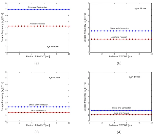
frequency values are independent of SWCNT diameter see Fig.(6), for all wave modes. The detailed variation in escape frequency for SWCNTs as a function of non-local scale parameter is shown in Figs. 6(a)-(d) fore0a=0.5nm, 1.0nm, 1.5nmand 2.0nm, respectively. It shows
the effect of the radius of the nanotube and nonlocal scaling parameter (e0) on the escape
frequency of SWCNTs more clearly. The escape frequencies for both axial and flexural modes are same that of the shear and contraction waves is also same and these are constant with respect to the radius of the CNT. These values of escape frequency are decreasing with the nonlocal scale coefficiente0a see Fig.6(a)-(d) and are still constant with radius of CNT.
The variation of the cut-off frequencies of shear contraction wavemodes with radius(R) of SWCNT are shown in Fig. (7). This figure shows that, as the radius of the nanotube increases, the cut-off frequencies decrease and at higher values ofR, the cut-off frequencies approach to a very small values. Hence, it can be concluded that for large values of scale parameter, shear deformation on CNT has negligible effect and CNT behaves like more like elementary beam.
0 2 4 6 8 10
0 1 2 3 4 5 6 7 8
Radius of SWCNT [nm]
Escape frequency (
ωe
) [THz]
Axial and Flexural Shear and Contraction
e 0a = 0.5 nm
(a)
0 2 4 6 8 10
0 1 2 3 4 5 6 7 8
Radius of SWCNT [nm]
Escape frequency (
ωe
) [THz]
Shear and Contraction
Axial and Flexural e
0a = 1.0 nm
(b)
0 2 4 6 8 10
0 1 2 3 4 5 6 7 8
Radius of SWCNT [nm]
Escape frequency (
ωe
) [THz]
Axial and Flexural Shear and Contraction
e0a = 1.5 nm
(c)
0 2 4 6 8 10
0 1 2 3 4 5 6 7 8
Radius of SWCNT [nm]
Escape frequency (
ωe
) [THz]
e 0a = 2.0 nm
Shear and Contraction
Axial and Flexural
(d)
0 2 4 6 8 10 0
5 10 15
Radius of SWCNT [nm]
Cut−off frequency [THz]
Contraction Mode Shear Mode
Figure 7 Cut-off frequency variation of the shear and contraction wave modes.
20 40
60 80
100 120
140
20 40 −20 0 20
(a)
20 40
60 80
100 120
140
20 40 −20 0 20
(b)
20 40
60 80
100 120 140
20 40 −20 0 20
(c)
20 40
60 80
100 120
140
20 40 −20
0 20
(d)
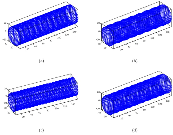
Fig. 8 shows the wave modes at 10.067 THz wave frequency of a (30,30) SWCNT of length 15.282 nm consisting of 7500 carbon atoms. Fig. 8a is for axial wave mode case, Fig. 8b is for contraction, Fig. 8c is for flexural and Fig. 8d is for shear wave modes of this SWCNT. From these figures one can clearly visualize the type of wave mode and its effect on the CNT.
Finally, wave propagation in CNTs has been a topic of great interest in nanomechanics, where the equivalent continuum models are widely used. In this manuscript, we examined this issue by incorporating the nonlocal theory into the classical model. The influence of the nonlocal effects has been investigated in details. The results are qualitatively different from those obtained based on the local/classical theory and thus, are important for the development of future CNT-based nanodevices.
4 CONCLUSIONS
The effect of nonlocal scaling parameter on the coupled wave propagation in single-walled car-bon nanotubes (SWCNTs) is studied.. The axial and transverse motion of SWCNT is modeled based on first order shear deformation theory and thickness contraction. The governing equa-tions are derived based on nonlocal constitutive relaequa-tions and the wave dispersion analysis is also carried out. The nonlocal elasticity calculation shows that the wavenumber tends to infinite at certain frequencies and the corresponding wave velocity tends to zero at those fre-quencies indicating localization and stationary behavior. A polynomial eigenvalue problem in wavenumbers is obtained as a function of wave frequency, nonlocal scale parameter and the material properties of the SWCNT. Explicit expressions are derived for cut-off and escape frequencies of all waves in SWCNT. It is also shown that the cut-off frequencies of shear and contraction mode are independent of the nonlocal scale parameter. The results provided in this article are useful guidance for the study and design of the next generation of nanodevices that make use of the wave propagation properties of single-walled carbon nanotubes.
References
[1] M. Born and K. Huang. Dynamical theory of crystal lattices. Clarendon Press, Oxford, 2002.
[2] A.N. Cleland. Foundation of nanomechanics. Sringer, 2002.
[3] J.F. Doyle. Wave propagation in structures. Springer-Verlag Inc. New York, 1997.
[4] A.C. Eringen. Linear theory of non-local elasticity and dispersion of plane waves.International Journal of Engineering Sciences, 10:425, 1972.
[5] A.C. Eringen. On differential equations of nonlocal elasticity and solutions of screw dislocation and surface waves.
Journal of Applied Physics, 54:4703, 1983.
[6] A.C. Eringen and D.G.B. Edelen. On non-local elasticity. International Journal of Engineering Sciences, 10:233, 1972.
[7] S. Gopalakrishnan. A deep rod finite element for structural dynamics and wave propagation problems. International Journal of Numerical Methods in Engineering, 48:731–744, 2000.
[8] S. Gopalakrishnan, A. Chakraborty, and D. Roy Mahapatra. Spectral finite element method. 2008.
[10] R.A. Jishi, L. Venkataraman, M.S. Dresselhaus, and G. Dresselhaus. Phonon modes in carbon nanotubules.Chemical Physics Letters, 209:77–82, 1993.
[11] M.R. Karim, M.A. Awal, and T. Kundu. Elastic wave scattering by cracks and inclusions in plates: in-plane case.
International Journal of Solids and Structures, 29(19):2355–2367, 1992.
[12] K.M. Liew and Q. Wang. Analysis of wave propagation in carbon nanotubes via elastic shell theories. International Journal of Engineering Sciences, 45:227–241, 2007.
[13] M. Mitra and S. Gopalakrishnan. Wave charecteristics of multi-walled carbon nanotubes. AIAA, page 1782, 2008.
[14] S. Narendar and S. Gopalakrishnan. Nonlocal scale effects on wave propagation in multi-walled carbon nanotubes.
Computational Materials Science, 47:526–538, 2009.
[15] J. Peddieson, G.R. Buchanan, and R.P. McNitt. Application of nonlocal continuum models to nanotechnology.
International Journal of Engineering Science, 41:305–312, 2003.
[16] Y.Z. Povstenko. The nonlocal theory of elasticity and its applications to the description of defects in solid bodies.
Journal of Mathematical Sciences, 97(1):3840–3845, 1999.
[17] A. Sears and R.C. Batra. Macroscopic properties of carbon nanotubes from molecularmechanics simulations, vol-ume 69. Physical Review B, 2004.
[18] L.J. Sudak. Column buckling of multiwalled carbon nanotubes using nonlocal continuum mechanics. Journal of Applied Physics, 94:7281–7287, 2003.
[19] L.F. Wang and H.Y. Hu.Transverse wave propagation in single-walled carbon nanotubes, volume 71. Physical Review B, 2005.
[20] Q. Wang. Wave propagation in carbon nanotubes via nonlocal continuum mechanics. Journal of Applied Physics, 98:124–301, 2005.
[21] E.W. Wong, P.E. Sheehan, and C.M. Lieber. Nanobeam mechanics: elasticity, strength, and toughness of nanorods and nanotubes. Science, 277:1971–1975, 1997.
[22] M. Xu. A one dimensional theory of compressional waves in an elastic rod. In Proceedings of First US National Congress of Applied Mechanics, pages 187–191, 1950.
[23] M. Xu. Free transverse vibrations of nano-to-micron scale beams. InProceedings of the Royal Society A: Mathemat-ical, Physical and Engineering Sciences, volume 462, pages 2977–2995, 2006.
[24] B.I. Yakobson, C.J. Brabec, and J. Bernholc. Nanomechanics of carbon tubes: Instabilities beyond linear response.
Physical Review Letters, 76:2511–2514, 1996.
[25] J. Yoon, C.Q. Ru, and A. Mioduchowski. Sound wave propagation in multiwall carbon nanotubes.Journal of Applied Physics, 93:4801, 2003.
[26] J. Yoon, C.Q. Ru, and A. Mioduchowski. Timoshenko-beam effects on transverse wave propagation in carbn nan-otubes. Composites Part B: Eng, 35:87–93, 2004.
[27] Y.Q. Zhang, G.R. Liu, and X. Han. Effect of small length scale on elastic buckling of multi-walled carbon nanotubes under radial pressure.Physics Letters A, 349(5):370–376, 2006.
[28] Y.Q. Zhang, G.R. Liu, and J.S. Wang. Small-scale effects on buckling of multiwalled carbon nanotubes under axial compression.Physical Review Letters, 70:205–430, 2004.
APPENDIX A: ELEMENTS OF MATRIX [Q]
The elements of the matrix [Q] given in Eq. (25 ) are
Q11=−C11J0k
2
+I0ω 2
+I0ω 2
(e0a) 2
k2
Q12=−Q21=−jC12J0k
Q13=Q31=0
Q14=Q41=C11J1k
2
−I1ω 2
−I1(e0a) 2
ω2k2
Q22=−C66J2k
2
−C12J0+I2ω 2
+I2ω 2
(e0a) 2
k2
Q23=Q32=−C66J1k
2
+I1ω 2
+I1ω 2
(e0a) 2
k2
Q24=−Q42=j(C66−C12)J1k
Q33=−C66J0k
2
+I0ω 2
+I0ω 2
(e0a) 2
k2
Q34=−Q43=jC66J0k
Q44=−C11J2k
2
−C66J0+I2ω 2
+I2ω 2
(e0a) 2
k2
(39)
APPENDIX B: ELEMENTS OF MATRIX [S2]
The elements of the matrix [S2] are
S2(11)=−C11J0+I0ω
2
(e0a) 2
S2(14)=S
(41)
2 =C11J1−I1(e0a) 2
ω2
S2(22)=−C66J2+I2ω
2
(e0a) 2
S2(23)=S
(32)
2 =−C66J1+I1ω 2
(e0a) 2
S2(33)=−C66J0+I0ω
2
(e0a) 2
S2(44)=−C11J2+I2ω
2
(e0a) 2