Universidade de Aveiro Ano 2011
Departamento de Física Departamento de Física
Susana Margarida
das Neves Mendes
FLUXOS CONVECTIVOS DE MOMENTO
LINEAR SIMULADOS POR UM MODELO
DE NUVENS 3D
FLUXOS CONVECTIVOS DE MOMENTO
LINEAR SIMULADOS POR UM MODELO
DE NUVENS 3D
FLUXOS CONVECTIVOS DE MOMENTO
LINEAR SIMULADOS POR UM MODELO
DE NUVENS 3D
CUMULUS MOMENTUM FLUXES IN
CLOUD-RESOLVING MODEL
SIMULATIONS OF TOGA-COARE
CUMULUS MOMENTUM FLUXES IN
CLOUD-RESOLVING MODEL
SIMULATIONS OF TOGA-COARE
CUMULUS MOMENTUM FLUXES IN
CLOUD-RESOLVING MODEL
Universidade de Aveiro Ano 2011
Departamento de Física Departamento de Física
Susana Margarida
Das Neves Mendes
FLUXOS CONVECTIVOS DE MOMENTO
LINEAR SIMULADOS POR UM MODELO
DE NUVENS 3D
FLUXOS CONVECTIVOS DE MOMENTO
LINEAR SIMULADOS POR UM MODELO
DE NUVENS 3D
FLUXOS CONVECTIVOS DE MOMENTO
LINEAR SIMULADOS POR UM MODELO
DE NUVENS 3D
CUMULUS MOMENTUM FLUXES IN
CLOUD-RESOLVING MODEL
SIMULATIONS OF TOGA-COARE
Dissertação apresentada à Universidade de Aveiro para cumprimento dos requisitos necessários à obtenção do grau de Doutor em Física, realizada sob a orientação científica do Doutor Christopher S. Bretherton, Professor Catedrático do Departamento de Ciências Atmosféricas da Universidade de Washington e do Doutor Alfredo Moreira Caseiro Rocha, Professor Associado com Agregação do Departamento de Física da Universidade de Aveiro
Apoio financeiro da FCT através de Bolsa de Doutoramento Refª
SFRH/BD22932/2005 no âmbito do III Q u a d r o C o m u n i t á r i o d e A p o i o (2000-2006).
o júri
presidente Professor Doutor José Carlos Esteves Duarte Pedro
Professor Catedrático da Universidade de Aveiro
Professor Doutor João Alexandre Medina Corte-Real
Professor Catedrático da Universidade de Évora
Professor Doutor Christopher S. Bretherton
Professor Catedrático da Universidade de Washington
Prof. Doutor Alfredo Moreira Caseiro Rocha
Professor Associado com Agregação da Universidade de Aveiro
Doutora Mariana Stichini Vilela Hart de Campos Bernardino
Investigadora do Instituto de Meteorologia
Doutor Paulo de Melo Gonçalves
agradecimentos Expresso aqui os meus mais profundos agradecimentos aos meus pais, que têm sido incansáveis e fonte de apoio inesgotável ao longo dos meus percursos pessoal e profissional. Obrigada por acreditarem e confiarem. Ao Professor Doutor Christopher S. Bretherton pela orientação e coordenação deste trabalho, pelo conhecimento transmitido e pela educação científica. Ao Prof. Doutor Alfredo Rocha pelo apoio fundamental, sob os mais diversos aspectos, ao longo de todo este processo.
Ao Professor Doutor João Corte-Real pela amizade, pela confiança, pela colaboração ao longo de mais de uma década e pelo contínuo estímulo dado em relação ao meu próprio percurso científico. Bem haja, Professor!
Aos Doutores Peter Blossey e Matthew Wyant, do Departamento de Ciências Atmosféricas da Universidade de Washington, pelas preciosas informações acerca dos dados, do modelo utilizado neste trabalho e pelas inúmeras dicas em relação ao software utilizado.
A todos os meus amigos, em Portugal e em Seattle, que me acompanharam sempre com muito carinho e inesgotável paciência, nesta longa jornada.
palavras-chave Transporte vertical de momento linear horizontal, convecção profunda, modelo de nuvens 3D, campanha TOGA-COARE.
resumo O objectivo deste trabalho científico é o estudo do transporte vertical de momento linear horizontal (CMT) realizado por sistemas de nuvens de convecção profunda sobre o oceano tropical. Para realizar este estudo, foram utilizadas simulações tridimensionais produzidas por um modelo explícito de nuvens (CRM) para os quatro meses de duração da campanha observacional TOGA COARE que ocorreu sobre as águas quentes do Pacífico ocidental. O estudo foca essencialmente as características estatísticas e à escala da nuvem do CMT durante um episódio de fortes ventos de oeste e durante um período de tempo maior que incluí este evento de convecção profunda. As distribuições verticais e altitude-temporais de campos atmosféricos relacionados com o CMT são avaliadas relativamente aos campos observacionais disponíveis, mostrando um bom acordo com os resultados de estudos anteriores, confirmando assim a boa qualidade das primeiras e fornecendo a confiança necessária para continuar a investigação. A sensibilidade do CMT em relação do domínio espacial do model é analisada, utilizando dois tipos de simulações tridimensionais produzidas por domínios horizontais de diferente dimensão, sugerindo que o CMT não depende da dimensão do domínio espacial horizontal escolhido para simular esta variável. A capacidade da parameterização do comprimento de mistura simular o CMT é testada, destacando as regiões troposféricas onde os fluxos de momento linear horizontal são no sentido do gradiente ou contra o gradiente. Os fluxos no sentido do gradiente apresentam-se relacionados a uma fraca correlação entre os campos atmosféricos que caracterizam esta parameterização, sugerindo que as formulações dos fluxos de massa dentro da nuvem e o fenómeno de arrastamento do ar para dentro da nuvem devem ser revistos. A importância do ar saturado e não saturado para o CMT é estudada com o objectivo de alcançar um melhor entendimento acerca dos mecanismos físicos responsáveis pelo CMT. O ar não saturado e saturado na forma de correntes descendentes contribuem de forma determinante para o CMT e deverão ser considerados em futuras parameterizações do CMT e da convecção em nuvens cumulus. Métodos de agrupamento foram aplicados às contribuições do ar saturado e não saturado, analisando os campos da força de flutuação e da velocidade vertical da partícula de ar, concluindo-se a presença de ondas gravíticas internas como mecanismo responsável pelo ar não saturado. A força do gradiente de pressão dentro da nuvem é também avaliada, utilizando para este efeito a fórmula teórica proposta por Gregory et al. (1997). Uma boa correlação entre esta força e o produto entre efeito de cisalhamento do vento e a perturbação da velocidade vertical é registada, principalmente para as correntes ascendentes dentro da nuvem durante o episódio de convecção profunda. No entanto, o valor ideal para o coeficiente empírico c*, que caracteriza a influência da força do gradiente de pressão dentro da nuvem sobre a variação vertical da velocidade horizontal dentro da nuvem, não é satisfatoriamente alcançado. Bons resultados são alcançados através do teste feito à aproximação do fluxo de massa proposta por Kershaw e Gregory (1997) para o cálculo do CMT total, revelando mais uma vez a importância do ar não saturado para
keywords Vertical transport of horizontal momentum, tropical deep convection, 3D cloud resolving model, TOGA-COARE campaign.
abstract The aim of the proposed research is the investigation of vertical cumulus momentum transport (CMT) in tropical oceanic deep convective cloud systems. Our approach is to use a unique four month three-dimensional cloud resolving model (CRM) simulations of TOGA COARE - a major field experiment over the warm waters of the west Pacific. Emphasis is given to the study of cumulus-scale characteristics of convective momentum transport during the December westerly wind burst and a longer time interval encompassing this specific deep convective event. The analysis of vertical and time-height distributions are evaluated against observations confirming the good quality and reliability of CRM simulations. Good agreement with previous studies is found. The CMT sensitivity to spatial domain size is analyzed using two data sets produced by different horizontal domain sizes, suggesting a non-dependency of this field upon the dimension of model spatial domain. The skill of the downgradient mixing-length parameterization is tested, highlighting the tropospheric regions where the momentum fluxes are downgradient and where they are upgradient. The upgradient transports are linked to an unexpected poor correlation between the fields involved in this parameterization, suggesting that formulations of updraft cloud mass flux and entrainment should be revisited. The role of saturated and unsaturated drafts on CMT is investigated in an attempt to reach a better understanding of their underlying physical mechanisms. The unsaturated air via downdrafts, and the saturated downdrafts have an important contribution to CMT, and they must be considered in future CMT and cumulus convection parameterizations. Binning methods are applied to these saturated and unsaturated contributions, through the analysis of buoyancy force and vertical velocity fields, suggesting the presence of internal gravity waves driving the unsaturated air. The cloud pressure-gradient force is also evaluated using the theoretical formula proposed by Gregory et al. (1997), exhibiting a strong correlation to the product mean vertical shear by vertical velocity perturbation, especially in cumulus updrafts during the strong convective event. However, an optimal value for the empirical coefficient c*, which characterizes the role of the cloud pressure-gradient force on the vertical variation of cloud horizontal velocity, is not satisfactorily achieved. Good results are accomplished by Kershaw and Gregory (1997) proposed mass flux approximation to total CMT, which has a fairly good performance in parameterization the total CMT and in identifying the regions of greater variability. Testing this particular approach revealed once again the important role of unsaturated air to the total CMT, which must be
Contents
List of Tables . . . ix List of Figures. . . . x 1 Introduction 231.1 Objectives of the Present Research . . . 23 1.2 An Overview of Convective Momentum Transport . . . 26 1.3 Convective Momentum Transport in TOGA-COARE observational
campaign . . . 29
2 The Cloud-Resolving Model and TOGA-COARE Simulations 33
2.1 The 3-dimensional cloud-resolving model . . . 33 2.2 Description of TOGA-COARE CRM simulations. . . 36
3 General Features of 3D CRM Simulations of TOGA-COARE 39
3.1 Time Series of CMT-relevant variables . . . 39 3.2 Comparison between small and large spatial domains of simulation . . . . 54
4 Mass-Flux Discretization of Convective Momentum Transport 59
4.1 Testing the SL76 scheme . . . 59 4.2 The relative CMT contributions from saturated and unsaturated air . . . . 68 4.3 Is the unsaturated CMT due to upward-propagating gravity waves? . . . . 78
5.1 Evaluating the role of the cloud pressure-gradient force . . .
Analysis of the perturbation pressure gradient acceleration on updrafts . . Julian Day 358 . . . Julian Days 350:359 . . . 85 86 88 94 5.2 The prediction of cumulus updrafts zonal velocity perturbation . . . . Julian Day 358 . . . . Julian Days 350:359. . . .
99 100 102 5.3 Testing the mass-flux approach to convective momentum transport
parameterization. . . . Julian Day 358 . . . . Julian Days 350:359. . . 104 105 109
6 Discussion and Directions for Future Work 115
ERRATA SHEET
This errata sheet lists errors and their correction for the doctoral thesis of Susana Margarida das Neves Mendes (nº 44786), titled “Cumulus Momentum Fluxes in Cloud-Resolving Model Simulations of TOGA-COARE”, Doctoral Program MAP-FIS, Department of Physics,University of Aveiro, October 2011.
Location Error Correction
Resumo, line 4 “por modelo” “por um modelo”
Resumo, line 20 “OS” “Os”
Resumo, line 37 “corficiente” “coeficiente”
Page x, 1.3, line 3 “reprrsents” “represents”
Page xi, 3.1.5, line 2 “TOGA-COAR” “TOGA-COARE”
Page xi, 3.1.9, line 1 “Total Cloud” “total cloud”
Page 24, par. 2, line 1 1977 1976
Page 24, par. 4, line 6 “Radar sets” “Radar data sets”
Page 25, par. 1, line 13 “ast” “last”
Page 26, par. 2, line 8 “bug” “big”
Page 31, par. 1, line 1 “-0.7” “0.7”
Page 34, par. 1, line 3 “os” “of”
Page 34, par. 2, line 15 “monotone” “monotonic”
Page 36, par. 2 , line 9 “Ciesielski” “Ciesielki (2003)”
Page 42, par. 2, line 2 “D256T120-S” “D256T10-S”
Page 42, par. 3, line 2 “120 day” “120-day”
Page 42, par. 3, line 2 “CRm” “CRM”
Page 46, par. 1, line 2 “vertical shear” “vertical wind shear”
Page 47, par. 2, line 10 “10-3” “10-3 (/s)”
Page 52, par. 1, line 3 “string” “strong”
Page 52, par. 1, line 6 “are” “area”
Page 53, par. 2, line 3 “et. Al” “et al”
Page 57, par. 1, line 7 “Figure 3.1.15” “Figure 3.2.2”
Page 61, par. 2, line 15 “(Fig. 3.1.18)” “(Fig. 3.1.12)”
Page 67, par. 1, line 1 “Table 4.1” “Table 4.1 and”
Page 69, par. 1 Paragraph repeated twice Delete the paragraph
Page 70, par. 4, line 9 “binning w” “binning”
Page 71, par. 1, line 6 “if” “If”
Page 72, par. 2, line 10 “levels” “level”
Page 78, par.1, line 5 “this” “This”
Page 79, eq. (4.3)
B
= T
T
d−
T
d
T
dB
= g
T
d−
T
d
T
d Page 79, eq. (4.5)B
= g −
T '
d
T
dB
= g
T '
d
T
dPage 79, par. 2, line 1 “Figures 4.2.8 and 4.2.9” “Figures 4.3.1 and 4.3.2”
Page 79, par. 3, line 3 “Figures 4.2.8, 4.2.9 and 4.2.10” “Figures 4.3.1, 4.3.2 and 4.3.3”
Page 83, par. 1, line 2 “and cloudy and” “and the air”
Page 83, par. 1, line 7 “(Fig. 4.2.2)” “(Fig. 4.3.2)”
Page 85, par. 2, line 2 “saturated” “unsaturated”
Page 91, par. 1, line 2
“cases, for both”
“cases, and for both”
Page 92, par. 1, line 3 “times” “time steps”
Page 110, par. 1, line 3 “fromc loud” “from cloud”
Page 117, par. 3, line 6 “environmental vertical velocity” “environmental zonal velocity”
Page 119, line 16 Missing reference Add:
Charney, J. G., and A. Eliassen, 1964: On the growth of
hurricane depression. J. Atmos.
Sci.,21, 68-75.
Page 122, line 8 Missing reference Add:
Palmen, E., and C. W. Newton, 1969: Atmospheric Circulations Systems. Academic, New York, 421 pp.
List of Tables
2.1 Brief summary of the relevant features of the data generated by the cloud-resolving model, and available for this thesis. . . 37
4.1 Slope values L (in meters) and correlation coefficients (in parentheses) for all tropospheric layers and all ∂z studied, as the result of applying a linear regression to the equation (4.2), for the two spatial domain data sets, D64T120-S and D256T10-S . . . 64
4.2 Definition of a saturated and unsaturated updraft model grid point, a saturated and unsaturated strong updraft model grid point, and a saturated and unsaturated downdraft model grid point, using its non-precipitating condensate (water plus ice) mixing ratio QN (g/kg) and its vertical velocity W (m/s) as defining characteristics. . . 69
List of Figures
1.1 Interactions between various processes in the climate system (from Arakawa, 2004) . . . 25
1.2 (a) Schematic diagram of the relative airflow and physical processes associated with a squall line mesoscale convective system. (From Moncrieff 1992, adapted from Houze et al. 1989).
(b) Schematic diagram of the airflow in the stationary dynamical model showing the three flow branches, namely jump updraught (A); downdraught (B); and overturning updraught (C), part of the archetypal model. (From Moncrieff 1992). . . 28
1.3 Measurement sites and study regions for the intensive observation period (IOP) of TOGA COARE. The legends beneath the panels refer to the symbols used to represent the observational platforms. This map reprrsents the entire COARE domain. The large-scale domain (LSD), the outer sounding array (OSA) and the intensive flux array (IFA) are outlined. (From Webster and Lukas 1992) . . . 30
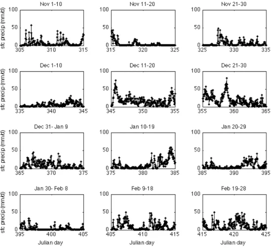
3.1.1 Surface precipitation (mm/day) for the whole period, 120 days, of
TOGA-COARE, given by the simulation D64T120-S . . . 43
3.1.2 The surface precipitation field (mm/day) for a 11-day period, from
December 20th to 30th, 1992, spatially averaged by the model over the
small domain 64 x 64 km2 . . . 44
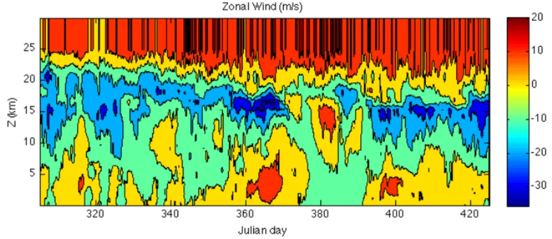
3.1.3 Time-height cross-section for zonal wind (m/s) during IOP, spatially
3.1.4 Time-height cross-section for zonal wind (m/s) provided by the simulation D64T10, a 3-D dataset, for a sub-period of 10 days, including the deep convective event occurred in December 24th . . . 45
3.1.5 Vertical profile of mean zonal wind simulated by D64T120-S, averaged over the whole 120-days of TOGA-COARE . . . 46
3.1.6 Vertical profile of the vertical wind shear (hr-1) simulated by the
D64T120-S dataset, averaged over the small domain and over TOGA-COARE IOP. . . 47
3.1.7 Time series of vertical wind shear (hr-1), given by simulation D64T120-S,
averaged over the whole atmospheric column . . . 48
3.1.8 Time-height cross-section of vertical wind (m/day), for the 10-day period, from Dec 16th to 25th, 1992, as simulated by the 3-D dataset
D64T10 . . . 49
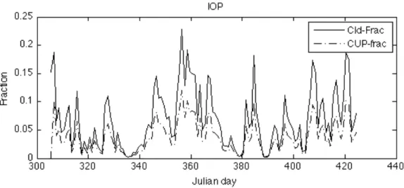
3.1.9 Time series of the Total Cloud area fraction (solid line) and the fractional area of cloudy updrafts (dash-dotted line), simulated by D64T120-S, for the whole TOGA-COARE period, 120 days. . . 49
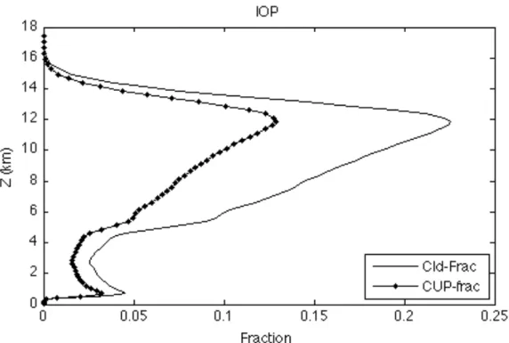
3.1.10 Vertical profiles of total cloud area fraction (solid line) and the fractional
area of cloudy updrafts (dotted line), as simulated by D64T120-S, averaged over IOP: 120 days . . . 50
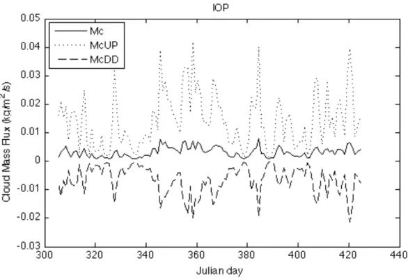
3.1.11 Time series of simulated total cloud mass flux (kg/m2/s, solid line), the
updraft cloud mass flux (dotted line, kg/m2/s) and the downdraft cloud
mass flux (dashed line, kg/m2/s), given by D64T120-S, for the
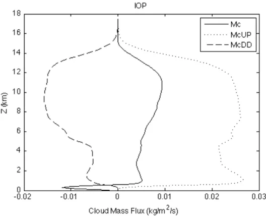
3.1.12 Vertical profiles of the total cloud mass flux (solid line), the updraft
cloud mass flux (dotted line) and downdraft cloud mass flux (dashed line), given by the D64T120-S dataset, averaged over the TOGA-COARE IOP . . . 52
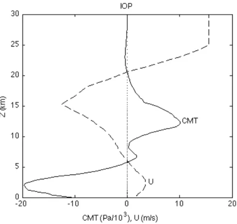
3.1.13 Vertical profiles of CMT (10-3 Pa) and mean zonal wind (m/s), provided
by D64T120-S dataset, averaged over the TOGA-COARE IOP . . . 53
3.2.1 Time series of surface precipitation (mm/hr), for the common 10-day period (Jd 350:359, December 16th to 25th, respectively), obtained by the
small domain simulation D64T120-S (Sd, dotted line) and by the large domain simulation D256T10-S (Ld, dashed line) . . . 55
3.2.2 Left: vertical profiles of mean zonal wind U (m/s/100), given by the
simulations D64T120-S (U64, small domain, starred solid line) and D256T10-S (U256, large domain, diamond solid line) and CMT (Pa), obtained by the simulations D64T120-S (CMT64, dotted line) and D256T10-S (U256, dashed line).
Right: vertical profiles of updraft cloud mass flux McUP64 and
McUP256 (kg/m2/s), of total cloud mass flux Mc64 and Mc256 (kg/m2/
s) and of downdraft cloud mass flux McDD64 and McDD256 (kg/m2/s),
provided by the small domain simulation D64T120-S and by the large domain simulation D256T10-S; averaged over the common 10-day period . . . . 56
3.2.3 Contour plots of time-height section of CMT (Pa) for the small domain
(top row left) and for the larger domain (top row right), and of total cloud mass flux Mc (kg/m2/s) given by D64T120-S (bottom row left)
and by D256T10-S (bottom row right), for the time interval Jd 350:359 . . . . 57
4.1.1 Hourly time series of X1 (Mcup*∂Ū/∂z, left column) and X2 (CMT, right column), for 10-day common period of simulation, within the lower, middle and upper troposphere, given by D64T120-S (dashed line) and D256T10-S (dotted line) data sets using the regular model vertical grid spacing ∂z. . . . 62
4.1.2 Daily time series of X1 (Mcup*∂Ū/∂z [Pa/m], left column) and X2 (CMT [Pa], right column), for 10-day common period of simulation, within the middle troposphere, for different choices of ∂z, given by D64T120-S (dashed line) and D256T10-S (dotted line) . . . 63
4.1.3 Scatter plots of X1 and -X2, and the linear regression applied to equation (4.2), for each ∂z, for small (circles and solid line) and large (diamonds and dotted line) domain sizes, within the lower troposphere . . . . 65
4.1.4 Scatter plots of X1 and -X2, and the linear regression applied to equation (4.2), for each ∂z, for small (circles and solid line) and large (diamonds and dotted line) domain sizes, within the middle troposphere . . . . 66
4.1.5 Scatter plots of X1 and -X2, and the linear regression applied to equation (4.2), for each ∂z, for small (circles and solid line) and large (diamonds and dotted line) domain sizes, within the upper troposphere . . . 67
4.2.1 Vertical profiles of the CMT (the product of the zonal wind perturbation (Up) by the vertical wind perturbation (Wp)) averaged over the eight 3D volumes from the small-domain simulation of Julian day 358, for the whole CRM spatial domain (solid-dotted line, both left and right plots), for the saturated (solid line, left plot) and unsaturated (solid line, right plot) domains, over the saturated and unsaturated updrafts (dashed line, left and right plots, respectively), over the strong saturated and unsaturated updrafts (dashed-two dots line, left and right
plots, respectively) and over the saturated and unsaturated downdrafts (dotted line, left and right plots, respectively) . . . 71
4.2.2 Vertical profile of unbinned CRM CMT (solid line) overlaid by the
binned CMT vertical profiles obtained by the bin sizes of 512 (dashed line), 256 (dashed-dotted line) and 128 (dotted line) elements, for Julian day 358 . . . . 72
4.2.3 Vertical profiles of the product of u' by w', averaged over the saturated
grid points (SAT), averaged over different number of bins examined for the saturated partition: 64 (Bs512, solid line), 128 (Bs256, dashed line), 256 (Bs128, dash-dot line) and 512 (Bs64, dotted line) . . . . 73
4.2.4 Vertical profiles of the product of u' by w', averaged over the
unsaturated grid points (UNSAT), averaged over different number of bins examined for the unsaturated partition: 64 (Bs512, solid line), 128 (Bs256, dashed line), 256 (Bs128, dash-dot line) and 512 (Bs64, dotted line) . . . 74
4.2.5 Scatter plots of binned u' and w', for specific bin sizes of 512 (left
column), 256 (mid-column) and 128 (right column) elements, at specific vertical levels of Z23 (3.625 km, top row), Z35 (6.625 km, second row), Z45 (9.125 km, third row) and Z62 (13.375 km, last row), with the correspondent coefficient of determination values (in %), given by D64T10 data set for eight 3D volumes of Julian day 358 . . . 75
4.2.6 Scatter plots of binned saturated (left column) and unsaturated (right
column) u' and w', for the bin size of 256 elements, at specific vertical levels of Z23 (3.625 km, top row), Z30 (5.375 km, second row) and Z35 (6.625 km, third row), with the correspondent coefficient of determination values (in %), given by D64T10 data set for eight 3D volumes of Julian day 358. . . 76
4.2.7 (continuation of Fig. 4.2.6) Scatter plots of binned saturated (left
column) and unsaturated (right column) u' and w', for the bin size of 256 elements, at specific vertical levels of Z45 (9.125 km, first row), and Z62 (13.375 km, second row) with the correspondent coefficient of determination values (in %), given by D64T10 data set for eight 3D volumes of Julian day 358. . . . 77
4.3.1 Scatter plots of binned saturated (left column) and unsaturated (right column) Buoyancy (By - circles - in m/s2), u’ (Up - dots - in m/s/100)
and w' (Wp in m/s), for the bin size of 256 elements, at specific vertical levels of Z23 (3.625 km, top row), Z30 (5.375 km, second row) and Z35 (6.625 km, third row), with the correspondent coefficient of determination values (in %), given by D64T10 data set for eight 3D volumes of Julian day 358. . . 80
4.3.2 (continuation of Fig. 4.3.1) Scatter plots of binned saturated (left
column) and unsaturated (right column) Buoyancy (By - circles - in m/ s2), u’ (Up - dots - in m/s/100) and w' (Wp in m/s), for the bin size of
256 elements, at specific vertical levels of Z45 (9.125 km, first row), Z62 (13.375 km, second row), Z72 (16.281 km) for saturated bins and Z83 (21 km, stratosphere) for unsaturated bins only, with the correspondent coefficient of determination values (in %), given by D64T10 data set for eight 3D volumes of Julian day 358. . . 81
4.3.3 Scatter plots of binned unsaturated Buoyancy (By - circles - in m/s2), u’ (Up - dots - in m/s/100) and w' (Wp in m/s), for the bin size of 256
elements, at specific vertical levels of Z33 (6.125 km, first plot), Z48 (9.875 km, second row), Z66 (14.81 km), with the correspondent coefficient of determination values (in %), given by D64T10 data set for eight 3D volumes of Julian day 358 . . . 82
5.1.1 Upper Left: vertical profile of the zonal wind perturbation Up (m/s)
averaged over the saturated updraft grid points and over the Julian day 358; Upper Right: time-height cross section of Up during the Jd 358, averaged over the saturated updraft grid points; Middle Left: vertical profile of the CMT (Pa) averaged over the saturated updraft grid points and over the Julian day 358; Middle Right: time-height cross section of
CMT during the Jd 358; Lower Left: zonal pressure-gradient force PGFx (m/s2) vertical profile average over the saturated updraft grid points and over the Jd 358, and Lower Right: time-height cross section of the PGFx during the Jd 358, averaged over the saturated updraft grid points. All quantities are provided by 3D D64T10 simulation. . . . 89
5.1.2 Upper Left: vertical profile of the zonal wind perturbation Up (m/s)
averaged over the saturated downdraft grid points and over the Julian day 358; Upper Right: time-height cross section of Up during the Jd 358, averaged over the saturated downdraft grid points; Middle Left: vertical profile of the CMT (Pa) averaged over the saturated downdraft grid points and over the Julian day 358; Middle Right: time-height cross section of CMT during the Jd 358; Lower Left: zonal pressure-gradient force PGFx (m/s2) vertical profile average over the saturated downdraft grid points and over the Jd 358, and Lower Right: time-height cross section of the PGFx during the Jd 358, averaged over the saturated downdraft grid points . . . 90
5.1.3 Left: vertical profiles of the mean vertical shear VWS (dotted line), of
the vertical velocity perturbation Wp (dashed line) and of the zonal cloud pressure-gradient force PGFx (solid line), averaged over the saturated updraft grid points and over the Julian day 358; Right: vertical profiles of the same fields, averaged over the saturated downdraft grid points and over the Jd 358. All quantities are provided by 3D D64T10 data set. . . . 91
5.1.4 Vertical profiles of the two members of equation (5.2) proposed by GKI97: the PGFx (m/s2, solid line) and the product of c* (0.7) by vertical velocity perturbation (m/s) by the mean vertical shear (/s) (dash line), averaged over the saturated updraft grid points (Left plot) and over the saturated downdraft grid points (Right plot), for Julian day 358. All the quantities are given by the 3D D64T10 simulation. . . . 92
5.1.5 Vertical profiles of the two members of equation (5.2) proposed by GKI97: the PGFx (m/s2, solid line) and the product of c* by vertical velocity perturbation (m/s) by the mean vertical shear (/s), considering several discrete choices for c*, averaged over the saturated updraft (Left plot) and over the saturated downdraft (Right plot) grid points, for Julian day 358. All the variables studied are given by the 3D D64T10 simulation. . . . 93
5.1.6 Linear regression applied to the equation (5.2) proposed by GKI97: the
PGFx as the predictand and the product of vertical velocity perturbation
Wp (m/s) by the mean vertical shear VS (/s) as the predictor, averaged
over the lower (left column, LT), the middle (mid-column, MT) and the upper (right column, UT) troposphere, within the saturated updraft grid points (first row) and over the saturated downdraft grid points (second row), for Julian day 358. All the quantities are given by the 3D D64T10 data set . . . . 94
5.1.7 Upper Left: vertical profile of the zonal wind perturbation Up (m/s)
averaged over the saturated updraft grid points and over the Julian days 350:359; Upper Right: time-height cross section of Up during the 10-day simulation, averaged over the saturated updraft grid points;
Middle Left: vertical profile of the CMT (Pa) averaged over the
saturated updraft grid points and over the Julian days 350:359; Middle
Right: time-height cross section of CMT during the 10-days; Lower Left: zonal pressure-gradient force PGFx (m/s2) vertical profile average over the saturated updraft grid points and over the 10-day period, and Lower Right: time-height cross section of the PGFx during the
10--days time period, averaged over the saturated updraft grid points. All quantities are provided by 3D D64T10 simulation . . . . 95
5.1.8 Upper Left: vertical profile of the zonal wind perturbation Up (m/s)
averaged over the saturated downdraft grid points and over the Julian days 350:359; Upper Right: time-height cross section of Up during the 10-days simulation, averaged over the saturated downdraft grid points;
Middle Left: vertical profile of the CMT (Pa) averaged over the
saturated downdraft grid points and over the Julian days 350:359;
Middle Right: time-height cross section of CMT during the 10-days; Lower Left: zonal pressure-gradient force PGFx (m/s2) vertical profile average over the saturated downdraft grid points and over the 10-days period, and Lower Right: time-height cross section of the PGFx during the 10-day time period, averaged over the saturated downdraft grid points. All quantities are provided by 3D D64T10 simulation. . . 96
5.1.9 10-day mean vertical profiles of the mean vertical shear VWS (dotted line, magnitude of 10-2), of the vertical velocity perturbation Wp
(dashed line), of the zonal cloud pressure-gradient force PGFx (solid line, magnitude of 10-2) of saturated updrafts (left) and saturated
downdrafts (right). All quantities are derived from 3D D64T10 simulation. . . 97
5.1.10 Vertical profiles of the two members of equation (5.2) proposed by
GKI97: the PGFx (m/s2, solid line) and the product of c* (0.7) by vertical velocity perturbation (m/s) by the mean vertical shear (/s) (dash line), averaged over the saturated updraft grid points (Left plot) and over the saturated downdraft grid points (Right plot), for the time period Jd 350:359. All the variables studied are given by the 3D D64T10 data set . . . . 98
5.1.11 Linear regression applied to the formula (5.2) proposed by GKI97: the PGFx as the predictand and the product of vertical velocity perturbation
Wp (m/s) by the mean vertical shear VS (/s) as the predictor, averaged
over the lower (left column, LT), the middle (mid-column, MT) and the upper (right column, UT) troposphere, within the saturated updraft grid points (first row) and within the saturated downdraft grid points (second row), for the time period Julian days 350:359. All the quantities are given by the 3D D64T10 simulation . . . 99
5.2.1 Vertical profiles of the CRM mean environmental wind Env (m/s, solid line), the cumulus updraft zonal velocity CRM Usup (m/s, circled line) simulated by the CRM and the parameterized cumulus updraft zonal velocity given by equation (5.1) assuming the action of entrainment only, discarding the contribution from the pressure-gradient force (m/ s, dashed line). All the profiles are given by the 3D D64T10 data sets . . . . 101
5.2.2 Left plot: vertical profiles of the CRM mean environmental wind Env
(m/s, solid line), the cumulus updraft horizontal velocity CRM Usup (m/s, circled line) simulated by the CRM and the parameterized cumulus updraft horizontal velocity given by equation (5.1), under different c* choices constant over height (m/s, colored lines). Right
plot: the same vertical profiles for environmental (solid line) and
simulated CRM zonal wind averaged over the cumulus updrafts (circled line), and the cumulus updraft zonal wind predicted by parameterization (5.1) using c* given by the linear regression slope. All data is given by the 3D D64T10 simulation . . . 102
5.2.3 Vertical profiles of the CRM mean environmental wind Env (m/s, solid
line), the cumulus updrafts horizontal velocity CRM Usup (m/s, circled line) simulated by the CRM and the parameterized cumulus updraft horizontal velocity given by equation (5.1) assuming the action of entrainment only, discarding the contribution from the pressure-gradient force (m/s, dashed line). All the profiles are given by the 3D D64T10 data sets and are averaged over the 10-day period . . . 103
5.2.4 Left plot: vertical profiles of the CRM mean environmental wind
‘Env’ (m/s, solid line), the cumulus updraft horizontal velocity ‘CRM Usup’ (m/s, circled line) simulated by the CRM and the parameterized cumulus updraft horizontal velocity given by equation (5.1), under different c* choices constant over height (m/s, colored lines). Right
plot: vertical profiles of the simulated cumulus updraft zonal wind
‘CRM Usup’ (circled line) and the parameterized cumulus updraft zonal wind with c* given by the linear regression slope. All data is given by the 3D D64T10 simulation and averaged over the 10-day time period . . . . 104
5.3.1 Left plot: vertical profiles of total cloud mass flux (kg/m2/s, solid line),
updraft cloud mass flux (kg/m2/s, dashed line) and downdraft cloud
mass flux (kg/m2/s, dotted line) given by the D64T120-S data set; Right plot: vertical profiles of total CMT (Pa, solid line), CMT within
cumulus updrafts (Pa, dashed line) and CMT within cumulus downdrafts (Pa, dotted line) given by the 3D data set D64T10 . . . . 106
5.3.2 Comparison between the CMT simulated by the cloud-resolving model
and the CMT given by equation (5.3). Left column: time-height cross sections of total CMT (top plot), cumulus updrafts CMT (middle plot) and cumulus downdrafts CMT (bottom plot) simulated by the 3D CRM.
Right column: time-height cross-section of total CMT (top plot), CMT
within cumulus updrafts (middle plot) and CMT within cumulus downdrafts (bottom plot) all obtained by the parameterization (5.3). White regions represent regions with no data. . . . 107
5.3.3 Vertical profiles of CRM (solid line) and parameterized (dotted lined)
CMT (Pa): total (left plot), within cumulus updrafts (mid-plot) and within cumulus downdrafts (right plot), for Julian day 358. . . . 108
5.3.4 Time-height cross-section of the ‘residual’ CMT, simulated by the
CRM, obtained as the difference between total CMT and CMT contributed by cumulus drafts, for Julian day 358. . . . 109
5.3.5 Left plot: vertical profiles of total cloud mass flux (solid line), updraft
cloud mass flux (dashed line) and downdraft cloud mass flux (dotted line) given by the D64T120-S data set; Right plot: vertical profiles of total CMT (solid line), CMT within cumulus updrafts (dashed line) and CMT within cumulus downdrafts (dotted line) given by the 3D data set; all profiles are averaged over the 10-day period . . . 110
5.3.6 CMT simulated by the 3D cloud-resolving model: time-height cross
sections of the CMT contributed by cumulus updrafts (top plot), cumulus downdrafts (middle plot) and total CMT (bottom plot). Data provided by the data sets D64T120-S and 3D D64T10, for the 10-day period of simulation . . . 111
5.3.7 CMT given by the mass-flux approximation (5.3): time-height cross sections of the CMT within cumulus updrafts (top plot), cumulus downdrafts CMT (middle plot) and total CMT (bottom plot). Data provided by the data sets D64T120-S and 3D D64T10, for the 10-day period of simulation . . . 112
5.3.8 Vertical profiles of CRM (solid line) and parameterized (dotted lined)
CMT (Pa): total (left plot), within cumulus updrafts (mid-plot) and within cumulus downdrafts (right plot), averaged over the 10-day window . . . . 113
5.3.9 Time-height cross-section of the ‘residual’ CMT, simulated by the
CRM, obtained as the difference between total CMT and CMT contributed by cumulus drafts, for the 10-day time interval . . . 113
List of Acronyms
CAM Community Atmosphere Model
CMT Convective Momentum Transport
CRM(s) Cloud-Resolving Model(s)
CRM CMT Convective Momentum Transport simulated by the Cloud-Resolving
Model
D256T10 Large Domain (256 x 256 km2) for a 10-day Time period 3D data set
D256T10-S Large Domain (256 x 256 km2) for a 10-day Time period 1D/2D data
set
D64T10 Small Domain (64 x 64 km2) for a 10-day Time period 3D data set
D64T120-S Small Domain (64 x 64 km2) for a 120-day Time period 1D/ 2D data
set
GCM Global Climate Model
GKI97 Gregory, Keshaw and Inness, 1997
IFA Intensive Flux Array
IOP Intensive Observational Period
MJO Madden-Julian Oscillation
OSA Outer Sounding Array
QBO Quasi-Biennal Oscillation
SAM System for Atmospheric Modeling
SL76 Schneider and Lindzen, 1976
TOGA-COARE Tropical Ocean-Global Atmosphere Coupled Ocean-Atmosphere
Response Experiment
VS, VWS Vertical Wind Shear
WWB(s) Westerly Wind Burst(s)
Chapter 1
Introduction
1.1 Objectives of the present research
The role of cumulus convection in the climate system is of great importance, particularly at low latitudes and in summertime over midlatitude continents. Cumulus convection is a primary control on precipitation and tropospheric latent heating. Tropical convective clouds systems generate two thirds of the global precipitation and the associated latent heating is a principal driver of the atmospheric circulation. Cumulus convection also creates extensive clouds that affect earth’s radiation budget, and vertically fluxes heat, moisture and other atmospheric constituents throughout the troposphere. It also induces vertical momentum fluxes, which will be the subject of this thesis.
Cumulus convection is a subgrid scale process; cumulus updrafts and downdrafts have width on the order of 1 km, much smaller than a climate model horizontal grid spacing of order 100 or more km. Thus cumulus convection needs to be parameterized (that is, its feedbacks with the grid-scale variables need to be represented in the climate model), which has proved to be a challenging problem. In addition to its interaction with large-scale circulations, cumulus convection interacts closely with other small-scale processes such as boundary-layer turbulence, cloud microphysics, and land-surface heterogeneity (Figure 1.1), adding to the parameterization challenge.
Most of the vertical transport of air within the tropical and subtropical troposphere is accomplished by a combination of deep (heavily precipitating) and shallow (lightly precipitating or nonprecipitating) cumulus convection. Deep and shallow cumulus convection frequently occurs in environments of large vertical wind shear. In these environments, convective updrafts can have a systematically different horizontal velocity Chapter 1 - Introduction
than convective downdrafts, resulting in a net vertical flux of horizontal momentum, or convective momentum transport (hereafter named by CMT). Because CMT is caused by small-scale updrafts and downdrafts, its average effect on global space and timescales cannot be measured directly. Hence, the effect of CMT on the global atmospheric circulation is still uncertain.
Studies of both idealized (e.g. Houze 1973, Schneider and Lindzen 1977), and general circulation (e.g. Zhang and McFarlane 1995) models have suggested that CMT has a important effect on mean zonal winds in the tropics and may also play a role in transient disturbances such as the Madden-Julian Oscillation (MJO), although few reliable observations exist over regions large enough to verify these modelling results. For these regions or larger scales, CMT can be inferred from an observational radiosonde network using a budget residual, although this involves considerable uncertainty deriving from the need to estimate the synoptic-scale pressure gradient force. Using this method, Carr and Bretherton, (2001) and Lin et al. (2005) showed over the western tropical Pacific, CMT tends to damp vertical wind shear in mean zonal winds or transient disturbances, such as the Madden-Julian Oscillation (MJO), on timescales of 5-10 days. It influences the tropical Hadley Circulation, rainfall and surface winds across the tropics (e.g. Richter and Rasch, 2008).
To represent these effects in climate models requires a parameterization of CMT. Diverse parameterizations have been proposed, but they are inadequately grounded in small-scale observations and modeling. The turbulent transport of momentum is different than for atmospheric constituents such as heat and moisture because due to pressure gradient forces, momentum is not conserved following fluid parcels even in the absence of mixing. Past studies suggest that even the sign of the transport depends on the degree and geometry of the cloud organization.
The major goal of this work is to improve our understanding of the vertical transport of horizontal momentum by deep convection over the tropical oceans, using a unique four month three-dimensional cloud-resolving model simulation of TOGA-COARE, a major field experiment over the warm waters of the west Pacific, characterized by extended periods of strong convection in strong vertical wind shear - ideal conditions for CMT, and extensive radiossonde, aircraft, and radar data sets which provide a good foundation for checking the quality of the CRM simulation. The author will investigate the statistical and the cumulus-scale characteristics of the convective momentum transport, examining the signs of the vertical transport of horizontal momentum during strong convection episodes, the sensitivity of CMT to grid resolution and domain size, the contribution from saturated and unsaturated up-and-downdrafts to CMT, and the accuracy of the physical assumptions made in some existing parameterizations of CMT. 1.1 Objectives of the present research
Figure 1.1. Interactions between various processes in the climate system (from Arakawa, 2004).
This dissertation will be structured in the following manner: Chapter 2 will briefly describe the cloud-resolving model used and the various TOGA-COARE simulations analyzed. In Chapter 3, the author will present time series of the most CMT-relevant variables and the comparison of CMT between two simulations characterized by different spatial domain sizes. Chapter 4 presents a test of the mass-flux approach to parameterization of CMT and evaluates the contribution of saturated and unsaturated up-and downdrafts to CMT. In Chapter 5, the author will discuss the prediction of U', the perturbation of the zonal component of the horizontal wind, and will evaluate the contribution of the pressure gradient force and entrainment terms for this prediction, assessing the issues related to these contributions. A direct comparison with the Gregory et al. (1997) CMT parameterization scheme using different choices for an adjustable coefficient called c* and the deduction of an optimal value for c*, defines the last section of Chapter 5. Chapter 6 will present a summary of the results, conclusions and directions for future work on the subject .
1.2 An Overview of Convective Momentum Transport
The first calculations using scale analysis and indirect estimates of vertical motion (e.g. Charney and Eliassen 1964, Palmen and Newton, 1969), suggested that CMT might be important to both steady and transient flows. Ooyama (1971) modelled CMT by assuming that momentum was mixed vertically like other scalars such as heat and moisture, and suggested that CMT should act to reduce the deep tropospheric shear in the environment. This transport is referred as downgradient transport, since momentum is transported from levels of high momentum to levels of low momentum. Schneider and Lindzen (1976) noted that even without turbulent mixing, the momentum of a cloud parcel can change during its ascent, due to cloud-scale pressure gradients produced by the relative horizontal motion of the cloud to its environment. This opened the possibility that CMT cloud act in a counter-gradient sense, that is, to increase the vertical shear. During the 1970s, large-scale budget studies provided the first substantial observational determination of CMT. These studies estimated momentum flux convergence as the residual of a horizontal momentum budget over an array of sounding stations. This budget included contributions from large-scale horizontal momentum advection and storage, from Coriolis forces, and from pressure gradient forces. The challenge in this approach is that the residual term is typically much smaller than the other terms, so small uncertainties in these other terms (especially the pressure grandient force) magnify into big uncertainties in the CMT. Larger-scale budget residual studies, despite uncertainties, also suggest mesoscale convective organization impacts CMT. Momentum budgets have been constructed for shallow (e.g. Holland and Rasmussen 1973) and deep convection (e.g. Stevens 1979, Wu and Yanai 1994). Stevens (1979) calculated the momentum budget in easterly waves over the tropical Atlantic Ocean, in which deep convection was often organized in north-south oriented squall lines. In the wave troughs, where the convection was most vigorous, the author found downgradient CMT in the along-line direction with little CMT in the across-line direction, an anisotropy consistent with in-situ observations of squall lines. The synoptic-scale pressure gradient force was a major uncertainty in this study. Wu and Yanai (1994) examined mesoscale convective systems observed by storm- and mesoscale sounding arrays in Oklahoma and Kansas. Upper-tropospheric environmental wind shear was reduced by CMT in a mesoscale convective complex case and increased in a squall line case, suggesting once more the existence of a relationship between CMT and convective organization.
Sui and Yanai (1986) tried to overcome the uncertainties in inferring CMT from a 1.2 An Overview of Convective Momentum Transport
momentum budget residual by using a vorticity budget approach, in which the pressure gradient force does not appear. The curl of the momentum flux convergence is a source of vorticity which can be deduced as a budget residual, but this still requires a number of assumptions about conditions along the perimeter of the budget domain and in practice does little to decrease the uncertainty of the derived CMT.
Direct eddy-correlation measurements made by aircrafts and using winds derived from dual-Doppler radar analysis in field campaigns contributed significantly to understanding convective momentum transport. In a seminal observational study of momentum fluxes in squall lines, LeMone (1983) showed that in the across-line direction, CMT can act to increase the environmental wind shear. The tilt of the updraft produced mesoscale horizontal pressure gradients around the leading edge of the line that accelerated the updrafts rearward and downdrafts forward. This pressure distribution was exactly opposite to that predicted by flow around an obstacle and suggests that cumulus momentum fluxes can depend at a considerable degree in the convective organization. Many observational (e.g. LeMone et al. 1984, Flatau and Stevens 1987, LeMone and Jorgenson 1991, Gallus and Johnson 1992), and modeling (e.g. Soong and Tao 1984, Lafore et al. 1988, Gao et al. 1990) studies have confirmed the existence of countergradient or ugradient momentum fluxes in organized systems, of the sign opposite that predicted by mixing-length theory. These studies suggest that depending on the vertical profile of horizontal wind U(z), two-dimensional convection in the atmosphere can transport U-momentum either up or down the vertical shear gradient, with the slope of the plane separating the leading-edge convection from the environment perhaps a better predictor of U-transport than the preceding environmental wind profile (the leading-edge is the intersection of a vertical plane normal to the convective line and the aforementioned plane). When the convective line is oriented to minimize the U shear (which is frequent), the evolution of U profile is such that the U-momentum is eventually countergradient.
It has been further found (LeMone et al. 1988a) that the CMT in a squall line is affected by the convection-induced perturbation pressure gradient resulting from the interaction between the main convective updraft and strong low tropospheric vertical shear of horizontal wind, as studied by Rotunno and Klemp (1982). However, in a 3D numerical study that included the neds of a squall line, Trier at al. (1998) found that the overall cross-line CMT was downgradient, even though was upgradient on the mid-plane. The convective-scale pressure perturbation is weaker in a low-shear environment, as observed by LeMone et al. (1988b). Therefore, nonsquall mesoscale convective systems that develop in a low-shear environment are unlikely to have upgradient CMT.
Figure 1.2. (a) Schematic diagram of the relative airflow and physical processes associated with a squall line mesoscale convective system. (From Moncrieff 1992, adapted from Houze et al. 1989). (b) Schematic diagram of the airflow in the stationary dynamical model showing the three flow branches, namely jump updraught (A); downdraught (B); and overturning updraught (C), part of the archetypal model. (From Moncrieff 1992).
Moncrieff (1992) developed an archetypical model which allowed for countergradient transport in organized systems by representing the effects of mesoscale circulations and the flow in the across-line direction by three branches: a descending downdraft, jump updraft, and overturning updraft (Figure 1.2). It is the dynamics and thermodynamics of the jump updraft responsible for the production of much of the countergradient transport. LeMone and Moncrieff (1993) found this model to be a good representation of line-normal CMT for quasi-two-dimensional convective bands, but its implementation as a parameterization of CMT in global models faces several challenges, e.g.: a) the closure for the model requires an assumption about the orientation of the convective lines which is not verified by observations, and b) as Trier et al (1998) study found, local countergradient transport in a squall line often does not generalize to larger space and timescales. Most current CMT parameterizations (e. g. Gregory 1997, Zhang and Cho 1991) are based on idealized models of flow partly entrained into and partly diverted around an isolated cumulus updraft. For most wind profiles, these parameterizations tend to produce largely downgradient fluxes, which result in a smoothing of the environmental wind profile.
1.3 Convective Momentum Transport in TOGA-COARE
observational campaign
The Tropical Ocean-Global Atmosphere Coupled Ocean-Atmosphere Response Experiment (TOGA COARE, Webster and Lukas 1992) provided an attractive opportunity to examine reanalysis-based estimates of convective momentum transport (CMT). The TOGA COARE Intensive Observation Period (IOP) took place over the tropical western Pacific from November 1st 1992 to February 28th 1993. During this period soundings were launched every six hours at four stations on the perimeter of the IFA: Kavieng (-2.35N, 150.48E), Kapingamarangi (1.04N,154.48E), R/V Kexue#1 (-4.00N,156.00E), and R/V Shigan#3 (-2.00N,158.00E). Soundings were also taken at a more coarsely spaced network of surroundings stations. Upper-air sounding stations were located at the vertices of an Intensive Flux Array (IFA, Figure 1.3), and at a larger Outer Sounding Array (OSA). Additional sounding stations were also scattered throughout the region.
The vertical transport of horizontal momentum by cumulus convection was investigated in observations and model simulations of the Tropical Ocean Global Atmosphere Coupled Ocean-Atmosphere Response Experiment (TOGA COARE). Estimates of CMT were obtained from radar data, momentum budget residuals, and two-dimensional cloud-resolving models and CMT parameterizations. During the “active” periods of strong deep convection, there was often strong, deep vertical wind shear, lending hope that cumulus momentum fluxes might be sufficiently large to reliably estimate from a budget approach. However, Carr and Bretherton (2001) concluded that budget estimates of CMT were strongly affected by pressure-gradient uncertainties, with no clearly detectable signature of CMT above 850 mb. Below 850 mb, there was a tendency for downgradient transport.
Using radar data, Houze et al. (2000) concluded that the nature of mesoscale CMT during COARE varied with the phase of the Madden-Julian Oscillation. Qualitatively, transport of mid-level momentum by mesoscale downdrafts appeared to be downgradient during the onset of a December westerly wind burst, but countergradient during the period of strongest low-level westerlies.
Tung and Yanai (2002a and 2002b) investigated the general features of CMT and analysed specific case studies during TOGA-COARE. In their Part I, using sounding data, taken during the IOP, they studied the CMT effects through the residual of the large-scale momentum approach and concluded that CMT exhibits a profound transient behavior, modulated by the MJO and other disturbances. They also noted that, on average, the Chapter 1 - Introduction
vertical momentum transport is downgradient. Using the same approach with a specific objective analysis (2002b), they investigated the CMT associated with several convective events during TOGA-COARE. Their findings confirmed the role of CMT in modulating the large-scale motions, but also suggested its role in modulating the multiscale interaction among large-scale waves of various periods. Their analysis is very sensitive to their assumed pressure fields, which are quite uncertain, as Carr and Bretherton pointed out.
Figure 1.3. Measurement sites and study regions for the intensive observation period (IOP) of TOGA COARE. The legends beneath the panels refer to the symbols used to represent the observational platforms. This map reprrsents the entire COARE domain. The large-scale domain (LSD), the outer sounding array (OSA) and the intensive flux array (IFA) are outlined. (From Webster and Lukas 1992).
Zhang and Wu (2003), through a month-long 2D CRM simulation of TOGA-COARE convective systems using the observed large-scale forcing, tried to understand the role of the convection-induced perturbation pressure field in the momentum transport. To quantify the performance of the mass flux approximation, they computed the vertical profiles of the linear regression slopes at each level and the correlation coefficients between the pressure gradient and the product of cloud mass flux and vertical wind shear. The slope was close to -0.4 in the lower troposphere and slightly larger in the upper 1.3 Convective Momentum Transport in TOGA-COARE observational campaign
troposphere, where they were forced to conclude that the value of 0.7 proposed by Gregory et al. (1997) was too large. They also showed that momentum transport by active convective downdrafts is small due to the weak downdraft mass flux. These authors noted that a 2D simulation, while more computationally affordable, may not be a good approximation for deriving CMT and pointed out that, long-term simulation with a 3D CRM should be the ultimate approach to investigate convective momentum transport in the future.
Chapter 2
The Cloud-Resolving Model and
TOGA-COARE Simulations
2.1 The 3-dimensional cloud-resolving model
Over the last decades, cloud-resolving models (CRMs) have been widely used as a tool to assist in the formulation and testing of cloud parameterization schemes for larger-scale models. There are several advantages in using CRMs over observational data, one of the most important is that clouds are explicitly represented. Better spatial and temporal resolution is achieved. It is assumed that CRMs are able to represent the main features of convective storms correctly. These models have some skill in simulating a wide variety of cloud structures, giving some confidence that there is value in using these data to develop convective parameterization schemes for use in large-scale models (Kershaw and Gregory, 1997).
Cloud-resolving models can be used to estimate the momentum transports by deep convection, for different flow regimes and cloud organizations. As well as providing estimates of the net transport of momentum, the CRMs simulations provide details of the internal cloud-structure, such as the variation of horizontal wind with height within cloud and the structure and magnitude of the cloud pressure-gradient force can be estimated directly. Although the use of CRMs to study convective momentum transport has been increasing, this use has been limited to hours-long simulations of individual convection cases, often under idealized initial conditions, with the exception of Gray (2000), who computed the momentum transport by mesoscale convective systems over a 6-day period Chapter 2 - The Cloud-Resolving Model and TOGA-COARE simulations
in TOGA-COARE. Two-dimensional CRMs distort the air flow through and around convective clouds too much to reliably simulate convective mass transport, often leading to simulation of squall-line organization and upgradient convective momentum transport not observed in a 3-dimensional CRM of the same convective environment. Like Zhang and Wu (2003) stated long-term 3D CRM simulations should be used to investigate CMT. Many authors (e.g. Moncrieff, 1992) have stressed the importance of organized mesoscale circulations within convective storms, which may require a large computational domain to simulate. Thus it is important to test the sensitivity of CRM-simulated CMT to domain size.
The simulations available to perform this study were provided by the System for Atmospheric Modeling (SAM, Version 6.3), a CRM developed by Marat Khairoutdinov at Colorado State University and described in detail in Khairoutdinov and Randall (2003). The model solved non-hydrostatic and anelastic equations for a 3-dimensional, rectangular, cartesian horizontal grid over a flat and homogeneous surface. SAM used a staggered C-grid, in which divergence and pressure are calculated at the same point in order to avoid spurious oscillations in the velocity field. Surface fluxes were computed using Monin-Obhukov similarity theory from specified sea surface temperatures (SSTs), wind speed, humidity and temperature at the first model level above the surface. The CRM predicted the time variation of the three velocity components u, v and w, pressure p, and the three thermodynamic variables, liquid-ice static energy sli, total non-precipitating water (vapor/cloud) qt, and precipitating water qr. sli and qt were adiabatically conserved even during vapor/liquid phase transitions but had sources due to the formation and evaporation of precipitation. The thermodynamic variables were transported with a monotonic advection scheme to prevent unphysical states associated with spurious oscillations.
The model used a single-moment bulk microphysical parameterization. Liquid–ice static energy was defined as sli = CpT + gz - Lcqliq - Lsqice , where Cp is the specific heat of dry air at constant pressure, T is the absolute temperature (in Kelvin), g is the gravitational constant, qliq is the mass mixing ratio of liquid phase hydrometeors, qice is the mass mixing ratio of ice phase hydrometeors, and Lc and Ls are the latent heats of condensation and sublimation, respectively. A diagnostic relationship based on temperature was used to differentiate the phases of non-precipitating hydrometeors (cloud liquid water and cloud ice) and precipitating hydrometeors (rain, snow and graupel). Cloud ice had a non-zero terminal velocity that depended on cloud ice water content and was derived from observations in Heymsfield (2003). A Smagorinsky-Lilly parameterization of subgrid turbulence (Smagorinsky 1963) was employed. No planetary boundary layer scheme, such as those used in global climate or weather models, was used 2.1 The 3-dimensional cloud-resolving model
for vertical diffusion.
The CRM used three types of thermodynamic forcings: volumetric forcings (large-scale horizontal advection of sensible energy and moisture), surface forcings (either prescribed surface latent and sensible heat fluxes, or a prescribed sea surface temperature along with sea surface pressure) and a mean vertical velocity Wls (detailed description in Blossey et al, 2008). The CRM radiation scheme was adapted from version 3 of the CAM (Community Atmosphere Model, a global climate model - GCM - from NCAR, the National Center for Atmospheric Research) provided for the CRM. Longwave and shortwave radiative heating rates transfer were computed in each model grid column approximately every three minutes. Water vapor, liquid water and the cloud ice (but not precipitating hydrometeors) were all radiative active.
Periodic boundary conditions were applied in the horizontal directions, and a rigid lid boundary condition was used at the top of the domain. The model vertical grid (in height coordinates) was composed of 96 layers, from surface to 30 km height, with grid spacings that increase smoothly from 75 m at the surface to a nearly uniform spacing of 250 m through the troposphere and then to 1 km in the Newtonian damping region, or sponge-region, in the top 30% of the model vertical domain, which prevented the reflection of upward-propagating gravity waves disturbances. In this damping region, perturbations of all prognostic variables from their horizontal mean were damped on a timescale that varies from two hours at 19 km to two minutes at the top of the domain. In the top two model layers, the mean thermodynamic profiles were nudged to specified observationally-derived profiles with a relaxation time scale of one hour.
The CRM generated two types of outputs, The first type, 3D outputs were instantaneous three-dimensional fields of basic model variables, including pressure (mbar), zonal wind component (m/s), meridional wind component (m/s), vertical wind component (m/s), pressure perturbation (Pa), radiative heating rate (K/day), absolute temperature (K), water vapor mixing ratio (g/kg), non-precipitating condensate (water plus ice) mixing ratio (g/kg) and precipitating water (rain plus snow) (g/kg). The second type, 2D/1D (referred hereafter as “statistics”) included horizontally-averaged variables and derived quantities such as vertical fluxes that were calculated within the CRM each time step, time-averaged and output periodically at a similar frequency as the 3D fields.