Geostatistical modeling of spatial variability of water retention curves

(1)

HESSD

5, 2491–2522, 2008

Geostatistical modeling of water

retention curves

H. Saito et al.

Title Page

Abstract Introduction

Conclusions References

Tables Figures

◭ ◮

Back Close

Full Screen / Esc

Printer-friendly Version

Interactive Discussion

Hydrol. Earth Syst. Sci. Discuss., 5, 2491–2522, 2008 www.hydrol-earth-syst-sci-discuss.net/5/2491/2008/ © Author(s) 2008. This work is distributed under the Creative Commons Attribution 3.0 License.

Hydrology and Earth System Sciences Discussions

Papers published inHydrology and Earth System Sciences Discussionsare under open-access review for the journalHydrology and Earth System Sciences

Geostatistical modeling of spatial

variability of water retention curves

H. Saito1, K. Seki2, and J. ˇSim ˚unek3

1

Department of Ecoregion Science, Tokyo University of Agriculture and Technology, Fuchu, Tokyo 183-8509, Japan

2

Faculty of Business Administration, Toyo University, Tokyo 112-8606, Japan 3

Department of Environmental Sciences, University of California, Riverside, CA 92521, USA

Received: 1 August 2008 – Accepted: 3 August 2008 – Published: 3 September 2008

Correspondence to: H. Saito (hiros@cc.tuat.ac.jp)

(2)

HESSD

5, 2491–2522, 2008

H. Saito et al.

Title Page

Tables Figures

◭ ◮

Back Close

Full Screen / Esc

Abstract

This study compares the performance of two geostatistical approaches, parametric and non-parametric, to evaluate the spatial distribution of water retention curves. Data used in this study were obtained from the Las Cruces trench site database that contains wa-ter retention data for 448 soil samples. In a commonly used parametric approach, 5

three standard water retention models, i.e. Brooks and Corey (BC), van Genuchten (VG), and log-normal (LN), were first fitted to each data set. For each model, a cross validation procedure was used to estimate parameters at each sampling location, al-lowing computation of prediction errors. In a rarely used non-parametric approach, a cross validation procedure was first used to directly estimate water content values for 10

eleven pressure heads at each sampling location and then the three water retention models were fitted using the same automated procedure to compute prediction errors. The results show that the non-parametric approach significantly lowered prediction er-rors for the VG model, while moderately reducing them also for the LN and BC models.

1 Introduction

15

It is well known that water flow in the vadose zone is strongly influenced by spatial variability of soil hydraulic properties and is thus subject to large uncertainties. Con-sequently, for example, predictions of soil moisture distributions in the vadose zone or estimates of contaminant arrival time to groundwater strongly rely on robust esti-mates of the spatial distribution of soil hydraulic parameters. However, since exhaustive 20

sampling is practically impossible in most cases, we always only have an incomplete knowledge of the spatial distribution of these parameters. Geostatistical interpolation techniques are therefore used to estimate unknown values of these parameters at un-sampled locations from available observations.

Unlike for water flow in saturated systems, predictions of variably-saturated water 25

(3)

HESSD

5, 2491–2522, 2008

H. Saito et al.

Title Page

Tables Figures

◭ ◮

Back Close

Full Screen / Esc

also on knowledge of water retention and hydraulic conductivity characteristics that are usually described by various functional forms. The water retention characteristic for a given soil is usually obtained by measuring a series of pressure head and water content data pairs on a core sample and then by fitting the constructed discrete curve using a simple common model with a closed-form function, such as the well-known van 5

Genuchten model (van Genuchten, 1980). Predictions of water flow in soils using the numerical model are thus greatly improved when the estimated hydraulic parameters adequately represent the highly nonlinear relationships between the water content, pressure head and hydraulic conductivity. Although accurate estimation of water re-tention curves (WRC) or their model parameters is rarely a goal of a study, it is one 10

of the most crucial steps in modeling water flow and solute transport in the vadose zone. It has also been known that the soil hydraulic parameters are not only soil-type dependent, but also spatial-location dependent.

Although some soil hydraulic model parameters have been derived in a purely em-pirical way, many studies are based solely on these parameters. For example, Zhu and 15

Mohanty (2002) averaged the widely used van Genuchten “parameters” to simulate large-scale infiltration and evaporation processes. In Oliveira et al. (2006), stochas-tic fields of “parameters” were generated using conditioning parameters to simulate variably-saturated water flow in soils. A common theme in these studies is that soil hydraulic parameters, regardless of their derivation, can be treated as meaningful pa-20

rameters. The question then arises whether or not we can consider these derived (i.e. averaged or randomly generated) parameters to be equivalent to those representing soil physical properties that are measured experimentally. To our knowledge, there have been no studies that would rigorously investigate this question.

This study therefore aims to quantify how well (or bad) the spatial distribution of soil 25

(4)

HESSD

5, 2491–2522, 2008

H. Saito et al.

Title Page

Tables Figures

◭ ◮

Back Close

Full Screen / Esc

parameters are then estimated directly for locations without measurements. In the second approach retention data (i.e. water contents for particular pressure heads) are first estimated geostatistically for locations without measurements and retention curve model parameters are then fitted to these estimated retention curves (Fig. 1). In this study, the former approach is referred to as the “parametric” (or P) approach, while the 5

latter is referred to as the “non-parametric” (or NP) approach. The performance of P and NP approaches to estimate the spatial distribution of WRC model parameters is then evaluated.

2 Materials and methods

2.1 Water retention data and models 10

The soil hydraulic properties (e.g. water retention curves) used in this study were obtained from the Las Cruces Trench Site database (Wierenga et al., 1989). The database was generated as part of a comprehensive field study conducted in southern New Mexico near Las Cruces for validating and testing numerical models of water flow and solute transport in the unsaturated zone (Wierenga et al., 1991). A 24.6-m long 15

by 6.0-m deep trench wall was excavated and a total of 450 samples were taken from nine layers. From each layer, 50 samples were taken for every 0.5 m. Soil samples (undisturbed and disturbed) were then analyzed in the laboratory for soil properties, such as the bulk density, the saturated hydraulic conductivity and the soil water reten-tion curve. Soil water retenreten-tion curves were determined at 448 sampling locareten-tions,u

i,

20

i=1, 2. . .448 (Fig. 2). At each location, the water contents,θ(u

i;hj), were measured

at eleven pressure heads, hj, j=1, 2. . .11, of 0, −10, −20, −40, −80, −120, −200,

−300, ₋1000, ₋5000, and ₋15 000 cm H₂O. While undisturbed soil cores were used for the wet range (₋300 cm to 0 cm), disturbed soil samples were used with a standard pressure plate apparatus for the dry range (₋15 000 cm to₋1000 cm). More details on 25

(5)

charac-HESSD

5, 2491–2522, 2008

H. Saito et al.

Title Page

Tables Figures

◭ ◮

Back Close

Full Screen / Esc

terization and infiltration experiments at this site have been analyzed in a number of studies, including recent articles by Rockhold et al. (1996), Oliveira et al. (2006) and Twarakavi et al. (2008).

Figure 2 shows the spatial distribution of observed saturated water contents (i.e. when the pressure head is equal to 0 cm orh₁) at the site. The saturated water content 5

data are, as expected, spatially heterogeneous with mean, maximum, and minimum values of 0.322, 0.529, and 0.218, respectively. Although not shown here, water con-tents measured for other pressure heads are also spatially heterogeneous. Figure 3 depicts experimental water retention curves obtained for seven di_fferent depths (z) at x=10.75 m. There are some discontinuities between water contents observed for 10

pressure heads of₋300 cm and₋1000 cm due to the di_fference in measurement pro-cedures (Hills et al., 1993). Not surprisingly, none of seven curves are identical. This confirms the importance of analyzing the spatial distribution of water retention curves at this site.

Water retention curves are usually approximated using one of the common analytical 15

models. These models are then used to estimate the relationship between the (unsat-urated) hydraulic conductivity and the water content using the pore-size distribution models (e.g. Mualem, 1976) as the soil-water retention curve is considerably easier and more accurate to measure than unsaturated hydraulic conductivities. Therefore, in this study, only water retention curve data are analyzed.

20

Among many available retention curve models, the Brooks and Corey (BC) model (Brooks and Corey, 1964), the van Genuchten (VG) model (van Genuchten, 1980), and lognormal pore size distribution (LN) model (Kosugi, 1996) are the most widely used analytical expressions to represent the dependence of the water content on the capil-lary pressure head for unimodal pore systems. Detailed discussions on the commonly 25

(6)

HESSD

5, 2491–2522, 2008

H. Saito et al.

Title Page

Tables Figures

◭ ◮

Back Close

Full Screen / Esc

The parameterS_e is an effective saturation defined as follows:

S_e(h)=θ−θr

θ_s−θ_r (1)

whereθ_sand θ_r are the saturated and residual water contents (m3m−3), respectively. As can be seen from Table 1, in addition toθ_sandθ_r, all three models require two other shape (or empirical) parameters, leading to a total of four parameters representing the 5

retention curve models.

An application of these water retention functions requires reliable estimates of the parameters for a soil of interest. While θs is relatively easy to obtain experimentally,

the other retention parameters usually have to be estimated indirectly by fitting the analytical function to the experimental water retention data using an optimization ap-10

proach, such as a non-linear least-squares minimization approach (e.g. implemented in the RETC code). In most optimization procedures, the performance is improved if the initial estimates are close to the “true” solution of the inverse problem. In other words, if initial estimates are too far from the “true” solutions, the solution may not converge to the global minimum but to the local minimum of the objective function. Seki (2007) re-15

cently developed a program code that uses a full-automatic procedure to estimate soil water retention model parameters. The program automatically selects initial estimates based on observations so that the user does not have to make his/her selections. De-tails of the approach will not be discussed in this paper, but, it should be noted that the full-automatic approach worked very well in most cases when applied to a number of 20

water retention data from the UNSODA database (Leij et al., 1996; Seki, 2007). Such an approach is especially attractive when a great number of retention curves needs to be fitted simultaneously.

2.2 Geostatistical theory

To estimate an unknown value of a given soil property at unsampled locations, a geo-25

(7)

Con-HESSD

5, 2491–2522, 2008

H. Saito et al.

Title Page

Tables Figures

◭ ◮

Back Close

Full Screen / Esc

sider the problem of estimating the value of a soil attributez (e.g. water content or soil hydraulic parameters) at an unsampled locationu_{, where} u_{is a vector of spatial} co-ordinates. The available information consists of values of the variablez at N locations u

i,i=1,2. . .N. All univariate kriging estimates are variants of the general regression

estimatez∗(u_{) defined as:} 5

z∗(u₎₋_m₍u₎₌

n(u₎

X

α=1

λα(u) [z(uα)−m(uα)] (2)

whereλ_α(u_{) is the weight assigned to datum} _z₍u

α) and m(u) is the trend component

of the spatially varying attribute (Goovaerts, 1997). In practice, only observations clos-est to u _{are retained, that is the} _n₍u_{) data within a given neighborhood or window} W(u_{) centered on} u_{, while the influence of those farther away are discarded (Saito} 10

and Goovaerts, 2000). One of the most common kriging estimators is ordinary kriging (or OK), which estimates an unknown value as a linear combination of neighboring observations:

z∗(u₎₌

n(u)

X

α=1

λOK_α (u₎_z₍u

α) (3)

In OK, unlike a constant value used in simple kriging, the mean (or trend) at each es-15

timation location (i.e. local mean,m(u_{)) is implicitly re-estimated. OK weights}_λOK_α _are determined so as to minimize the error or estimation varianceσ2(u₎₌_{V arZ}∗₍u₎₋_Z₍u₎ under the constraint of an unbiased estimate (Goovaerts, 1997). These weights are obtained by solving the system of linear equations known as the ordinary kriging sys-tem:

20

    

   

n(u)

P β=1

λOK_β (u₎₌_γ₍u

α−uβ)+µOK(u)=γ(uα−u)α=1, . . ., n(u) n(u₎

P β=1

λOK_β (u₎₌₁

(8)

HESSD

5, 2491–2522, 2008

H. Saito et al.

Title Page

Tables Figures

◭ ◮

Back Close

Full Screen / Esc

where µ_OK(u_{) is the Lagrange parameter,} _γ₍u

α−uβ) is the semivariogram between

observations at u_α _and u_β_{, and} _γ₍u_α₋u_{) is the semivariogram between the datum} location u

α and the location being estimatedu. The semivariogramγ(h) models the

variability between observations separated by a vectorh_{. The only information required} by the system (Eq. 4) is the semivariogram values,γ, for di_fferent separation distances. 5

These values are readily derived from the semivariogram model fit to experimental values (i.e. linear model of regionalization):

ˆ

γ(u₎₌ 1 2N(h₎

n(u₎

X

α=1

[z(u

α)−z(uα+h)]2 (5)

whereN(h_{) is the number of data pairs for a given separation vector} h_{. The choice} of the model is limited to functions that ensure a positive definite covariance function 10

matrix of the left-hand-side of the kriging system (Eq. 4). Spatial correlations often vary with direction, and such a case requires one to compute semivariograms in di_fferent orientations and fit anisotropic (direction-dependent) semivariogram models. Details of model fitting can be found in Deutsch and Journel (1998), Goovaerts (1997), and Kitanidis (1997).

15

2.3 Prediction performances: P vs. NP

To compare the P and NP approaches in terms of reproduction of WRC,S_e(h;u

i), two

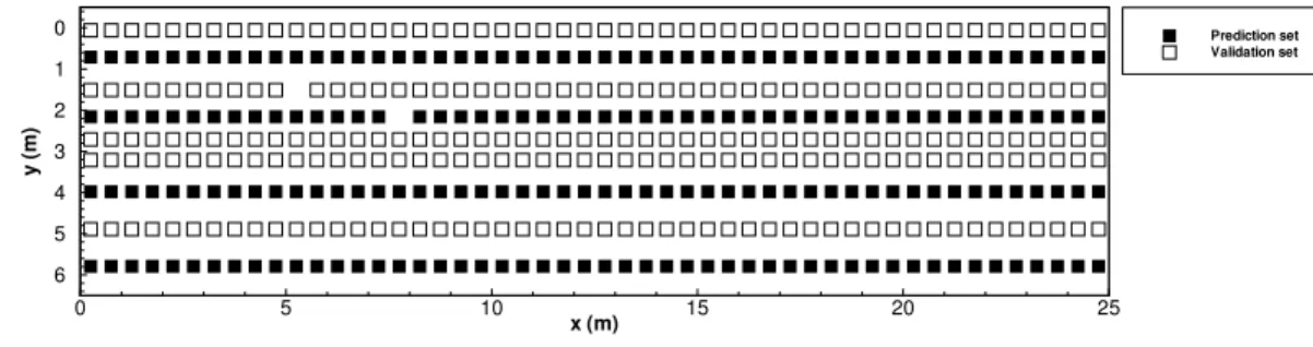
standard validation techniques were used: a cross-validation, in which one observa-tion at a time is temporarily removed from the dataset and re-estimated from remaining data, and a jack-knife, in which the dataset is divided into two non-overlapping pre-20

diction and validation sets (Fig. 4). The number of observation locations held in each set is 199 (Np) and 249 (Nv), respectively. In the jackknife technique, the prediction

(9)

HESSD

5, 2491–2522, 2008

H. Saito et al.

Title Page Abstract Introduction Conclusions References Tables Figures ◭ ◮ ◭ ◮ Back Close

Full Screen / Esc

WRC models, i.e. BC, VG, and LN, were considered. For both approaches, unknown values were estimated using ordinary kriging (Eq. 3). Note that, regardless of the ap-proach, semivariogram models used in kriging are those fitted to semivariograms for all 448 observations. Details about P and NP approaches used in this study are given below.

5

2.3.1 Parametric approach (P)

1. Parameters for three water retention functions (BC, VG, and LN) are first obtained for all 448 water retention curves S_e(h;u

i) using the automatic fitting procedure

(Seki, 2007).

2. For each soil hydraulic parameter, unknown values are estimated at all 448 loca-10

tions for the cross-validation and at 249 locations for the jackknife using ordinary kriging (OK).

3. For each model, a discrepancy between observed water retention curvesS_e(h;u

i)

and those calculated from estimated parametersS_e(h;u

i) is obtained at each

lo-cation by computing di_fferences in water contents at corresponding eleven pres-15

sure heads. Mean absolute error (MAE) and mean square error (MSE) are used in this study

MAE₌1 N

N X

i=i   1 11 11 X

j=1

|θˆ(u_i_;_h_j₎₋_θ₍u_i_;_h_j₎_|



 (6)

MSE=1 N

N X

i=i   1 11 11 X

j=1

( ˆθ(u

i;hj)−θ(ui;hj))2 

 (7)

whereN is 448 for the cross-validation and 249 for the jackknife, ˆθ(u

i;hj) is the water

20

(10)

HESSD

5, 2491–2522, 2008

H. Saito et al.

Title Page

Tables Figures

◭ ◮

Back Close

Full Screen / Esc

h_j, andθ(u

i;hj) is the observed water content at the locationui for the pressure head

hj.

2.3.2 Non-parametric approach (NP)

1. Unknown water content values corresponding to eleven pressure heads are esti-mated using OK at 448 locations for the cross-validation and 249 locations for the 5

jackknife.

2. Using the automatic fitting procedure (Seki, 2007), parameters for three WRC models (i.e. BC, VG, and LN) are obtained at each estimated location.

3. For each model, a discrepancy between observed water retention curves and those calculated from parameters obtained in the previous step is obtained by 10

computing MAE and MSE as done for the P approach.

4. The impact of the number of data pairs to construct WRC when estimating param-eters is investigated by repeating 1 through 3 using only the following six pressure heads: 0,₋20,₋80,₋200,₋1000, and₋15 000 cm. This approach is referred to as NP6 in the remainder of the paper, while the approach that considers all eleven 15

pressure heads is referred to as NP11.

3 Results and discussions

The results are divided into two sections. The first section summarizes experimental semivariograms computed from water retention data and model parameters. In the second section, different approaches (P and NP) are compared in terms of describing 20

(11)

HESSD

5, 2491–2522, 2008

H. Saito et al.

Title Page

Tables Figures

◭ ◮

Back Close

Full Screen / Esc

3.1 Semivariograms

Figure 5 shows the experimental semivariograms of WRC model parameters with fit-ted geometric anisotropy models. Semivariograms of water contents corresponding to eleven pressure heads,h₁–h₁₁, with fitted geometric anisotropy models are depicted in Fig. 6. All these semivariograms were calculated for 448 observations. Except forα_v 5

there is clear anisotropy in all semivariograms with major spatial continuity observed in the horizontal direction. While horizontal semivariograms, in general, are all well struc-tured, vertical semivariograms in most cases fluctuate a lot and are not smooth. There is not a sufficient number of pairs in the vertical direction to obtain well structured semi-variograms. Existence of soil horizons would also not result in spatial correlation of soil 10

variables in the vertical direction at the scale of observations. All experimental semi-variograms were fitted using either exponential or spherical models and they all display a clear nugget e_ffect. Ranges and sill values vary depending upon the variable. For example, as expected, semivariograms for the saturated (θ_s) and residual (θ_r) volumet-ric water contents are all similar for all three models (Fig. 5, top two rows). However, 15

other parameters have semivariograms of di_fferent shapes, which was expected as the spatial variability of these parameters varies.

As for the semivariograms of water contents at given pressure heads (Fig. 6), the ranges of water contents near saturation in the horizontal direction (i.e. major range) are generally larger than those for drier conditions. This suggests that the spatial conti-20

nuity of larger pores is more profound than that of smaller pores. When pressure heads are smaller than₋40 cm, the shape of the semivariograms becomes almost identical. From the Laplace equation for the capillary rise, the radius of the pore corresponding to the pressure head of₋40 cm can be calculated to be about 0.35 mm (assuming that the contact angle is equal to 0◦). Therefore, it can be concluded that spatial distributions of 25

(12)

HESSD

5, 2491–2522, 2008

H. Saito et al.

Title Page

Tables Figures

◭ ◮

Back Close

Full Screen / Esc

3.2 Prediction performance

Using both parametric and non-parametric approaches, water retention curve models can be geostatistically estimated at any location. Figure 7 shows differences between P and NP approaches in terms of predicting a water retention curve at a given loca-tion using the LN model. In this example, a localoca-tion where observed retenloca-tion data 5

(squares) were available was selected to investigate whether or not one approach out-performs the other in terms of reproducing the WRC. Due to the exactitude property of kriging, data at this location were not included in kriging. While the blue line is obtained with parameters predicted by the P approach, the red line is calculated with parame-ters obtained by the NP approach. In the P approach, model parameparame-ters were directly 10

estimated using OK from surrounding conditioning parameters. In the NP approach, the water retention curve was geostatistically constructed by estimating water content values corresponding to eleven pressure heads,h₁–h₁₁. Geostatistically constructed water retention data are shown in Fig. 7 using triangles. The LN model (the solid red line in Fig. 7) was then fitted to the predicted retention data to obtain model parameters. 15

While the model predicted using the P approach could not reproduce theS-shape ob-served in retention data, the model obtained using the NP approach could capture the trend of WRC well. This confirms that depending upon the chosen approach, resulting WRC models can be significantly different. In the following section, both approaches were compared in a more comprehensive manner using cross-validation.

20

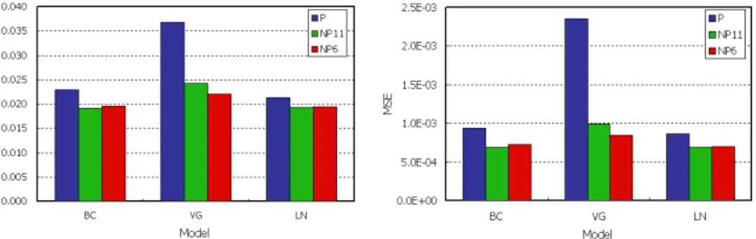
Figures 8 and 9 depict mean absolute errors (MAE) and mean square errors (MSE) calculated for all three approaches, i.e. P, NP11, and NP6, using cross-validation and jack-knife procedures for all three WRC models. In general, the NP approach resulted in smaller prediction errors regardless of the used WRC model, except when the LN model was used in the jack-knife procedure. Decreases in prediction errors were much 25

(13)

HESSD

5, 2491–2522, 2008

H. Saito et al.

Title Page

Tables Figures

◭ ◮

Back Close

Full Screen / Esc

parameterα_v(=28.16) was three orders of magnitude greater than the rest, where the mean of fitted αv is 0.12 and the median is 0.04 (Fig. 10). Although the fitting itself

was good at this particular location (Fig. 11), the largeα_v value (outlier) a_ffected the estimation ofα_v values at surrounding locations leading to relatively poor performance of the P approach for the VG model. This kind of problem can be avoided if the NP 5

approach is used. For the other two WRC models, average prediction errors decreased by about 10–15% when the NP approach was used compared to prediction errors for the P approach, in which there were no outliers in initially estimated parameters.

For the P approach, prediction errors vary depending upon the WRC model used. On the other hand, prediction errors do not depend upon the model used for the NP 10

approach. This is not a surprising result since in the NP approach three models were fitted to the same reconstructed WRCs. Therefore, all prediction errors calculated for the NP approach are mainly the summary of model fitting results but do not directly reflect the accuracy of geostatistical estimation as those for the P approach.

There is no distinct trend in whether or not the NP11 approach is better than NP6 15

or vice versa. While NP6 outperforms NP11 when the VG model is used, NP11 has slightly smaller average errors or almost the same errors compared to NP6 for the BC and LN models. This indicates that reducing the number ofθ−h pairs by about half does not necessarily worsen prediction performances as long as the non-parametric approach is adopted. This result is quite important since the main reason for the P 20

approach to be preferred over the NP approach in most studies is that the number of variables one needs to analyze can be significantly reduced. The number of parame-ters required in the WRC models used in this study is four, which is significantly smaller than original elevenθ−hpairs used to construct water retention curves. To use all pairs in the NP approach, one needs to perform kriging eleven times, which requires signifi-25

(14)

HESSD

5, 2491–2522, 2008

H. Saito et al.

Title Page

Tables Figures

◭ ◮

Back Close

Full Screen / Esc

description of the spatial variability of water retention curves using the NP approach. Figures 12 and 13 show spatial distributions of locations where NP11 outperformed P and vice versa in terms of MAE and MSE, respectively, in cross-validation. There is no specific trend observed, such as, for example, a cluster of white or black squares. This means that the prediction of water retention curves was fairly unbiased. Propor-5

tions of white squares for both NP11 and NP6 (spatial distributions are not shown) are summarized in Table 2 for all cases. For all models, the non-parametric approaches outperformed the parametric approach at more than 60% of sampling locations. Es-pecially for the VG model, the NP approaches resulted in smaller prediction errors at more than 80% of sampling locations. Although the difference between NP11 and NP6 10

is small, NP11 was slightly better than NP6 for BC and LN,, while NP6 was better than NP11 for VG. Overall, these percentages confirm the superiority of the NP approach to predict WRCs.

4 Conclusions

This study compares the performance of two geostatistical approaches, commonly 15

used parametric (P) and newly proposed non-parametric (NP), to estimate the spa-tial distribution of water retention curve parameters. In the former approach retention curve model parameters are first evaluated at sampled locations from observed reten-tion data and these parameters are then estimated directly for locareten-tions without mea-surements. In the latter approach retention data are first estimated using kriging for 20

locations without measurements and retention curve model parameters are then fitted to these estimated retention curves. Standard validation techniques (cross-validation and jackknife) were used to compare two approaches in terms of estimation of the spatial distribution of water retention curves.

Both validation results showed that regardless of the retention model selected, the 25

(15)

pa-HESSD

5, 2491–2522, 2008

H. Saito et al.

Title Page

Tables Figures

◭ ◮

Back Close

Full Screen / Esc

rameters led to the poor estimate of that parameter at surrounding locations in the P approach. There is always a risk of including parameter outliers in the estimation pro-cess as long as the P approach is used. In the NP approach, such a problem hardly occurs. In addition, the NP approach performed better than the P approach even when the number of data pairs used to construct retention curves was reduced from eleven to 5

six. This makes the NP approach comparable to the P approach in terms of workload because the number of variables used in the P approach is four, while that of the NP approach now becomes only 6. The P approach has been preferred mainly because one can reduce the computational time and workload. However, as this study shows, with a little bit of extra work, one can achieve much better estimation of the spatial 10

distribution of water retention curves by using the NP approach.

Overall, this study shows the superiority of the NP approach over the P approach to evaluate the spatial distribution of water retention curves, which is the initial but critical step to model variably-saturated water flow and solute transport in field-scale heterogeneous soils. In future studies, the actual impact of the NP approach on water 15

(16)

HESSD

5, 2491–2522, 2008

H. Saito et al.

Title Page

Tables Figures

◭ ◮

Back Close

Full Screen / Esc

References

Deutsch, C. V. and Journel, A.: GSLIB: Geostatistical Software Library and User’s Guide, Ox-ford Univ. Press, New York, 384 pp., 1998.

Hills, R. G., Wierenga, P., Luis, S., McLaughlin, D., Rockhold, M., Xiang, J., Scanlon, B., and Wittmeyer, G.: INTRAVAL – Phase II model testing at the Las Cruces Trench Site, Tech. rep.,

5

US Nuclear Regulatory Commission – NUREG/CR-6063, Washington, D.C., 140 pp., 1993. Goovaerts, P.: Geostatistics for Natural Resources Evaluation, Oxford Univ. Press, New-York,

483 pp., 1997.

Kitanidis, P. K.: Introduction to Geostatistics: Applications in Hydrogeology, Cambridge Univer-sity Press, New York, 271 pp., 1997.

10

Leij, F. J., Alves, W. J., van Genuchten, M. T., and Williams, J. R.: The UNSODA-Unsaturated Soil Hydraulic Database. User’s manual Version 1.0, Report EPA/600/R-96/095, National Risk Management Research Laboratory, Office of Research and Development, US Environ-mental Protection Agency, Cincinnati, OH, 103 pp., 1996.

Leij, F. J., Russell, W. B., and Lesch, S. M.: Closed-Form Expressions for Water Retention and

15

Conductivity Data, Ground Water, 35(5), 848–858, 1997.

Oliveira, L. I., Demond, A. H., Abriola, L. M., and Goovaerts, P.: Simulation of solute trans-port in a heterogeneous vadose zone describing the hydraulic properties using a multistep stochastic approach, Water Resour. Res., 42, W05420, doi:10.1029/2005WR004580, 2006. Rockhold, M. L., Rossi, R. E., and Hills, R. G.: Application of similar media scaling and

condi-20

tional simulation for modeling water flow and tritium transport at the Las Cruces Trench Site, Water Resour. Res., 32(3), 595–609, 1996.

Saito, H. and Goovaerts, P.: Geostatistical interpolation of positively skewed and censored data in a dioxin contaminated site, Environ. Sci. Technol., 34(19), 4228–4235, 2000.

Seki, K.: SWRC fit - a nonlinear fitting program with a water retention curve for soils having

25

unimodal and bimodal pore structure, Hydrol. Earth Syst. Sci. Discuss., 4, 407–437, 2007, http://www.hydrol-earth-syst-sci-discuss.net/4/407/2007/.

Twarakavi, N. K. C., Saito, H., ˇSim ˚unek, J., and van Genuchten, M. T.: A New Approach to Estimate Soil Hydraulic Parameters using Only Soil Water Retention Data, Soil Sci. Soc. Am. J., 72(2), 471–479, 2008.

30

(17)

HESSD

5, 2491–2522, 2008

H. Saito et al.

Title Page

Tables Figures

◭ ◮

Back Close

Full Screen / Esc

Interactive Discussion van Genuchten, M. T., Lesch, S. M., and Yates, S. R.: The RETC code for quantifying the

hydraulic functions of unsaturated soils, Version 1.0, US Salinity Laboratory, USDA, ARS, Riverside, CA, 93 pp., 1991.

Wierenga, P. J., Toorman, A. F., Hudson, D. B., Vinson, J., Nash, M., and Hills, R. G.: Soil physical properties at the Las Cruces trench site, NUREG/CR-5441, Nucl. Regul. Comm.,

5

Washington, D. C., 92 pp., 1989.

Wierenga, P. J., Hills, R. G., and Hudson, D. B.: The Las Cruces trench site: characterization, experimental results, and one-dimensional flow predictions, Water Resour. Res., 27, 2695– 2705, 1991.

Zhu, J. and Mohanty, B. P.: Spatial averaging of van Genuchten hydraulic parameters for

10

(18)

HESSD

5, 2491–2522, 2008

H. Saito et al.

Title Page

Tables Figures

◭ ◮

Back Close

Full Screen / Esc

Table 1.Water retention,S_e, models used in this study.

Models Expression Parameters

Brooks and Corey S_e(h)= (

1 h≤h_b

(_hh

b)

−λ _h>h

b

h_b[cm]

λ[−]

van Genuchten S_e(h)=_[1₊_|_αh1_|n

]m

n[−]

αg cm−1]

m(=1−1/n) [−]

Kosugi S_e(h)=12erf c n_ln(h/h

l)

√ 2σ

o h_l[cm]

(19)

HESSD

5, 2491–2522, 2008

H. Saito et al.

Title Page

Tables Figures

◭ ◮

Back Close

Full Screen / Esc

Table 2. Percentages (%) of locations where predictions errors (MAE and MSE) for the NP approach were smaller than those for the P approach in cross-validation.

Model BC VG LN

NP11 NP6 NP11 NP6 NP11 NP6

MAE 71.7 70.1 81.0 82.1 62.1 59.4

(20)

HESSD

5, 2491–2522, 2008

H. Saito et al.

Title Page

Tables Figures

◭ ◮

Back Close

Full Screen / Esc

(21)

HESSD

5, 2491–2522, 2008

H. Saito et al.

Title Page

Tables Figures

◭ ◮

Back Close

Full Screen / Esc

Interactive Discussion x (m)

z(

m

)

0 5 10 15 20 25

0 1 2 3 4 5 6 0 cm 0.42 0.4 0.38 0.36 0.34 0.32 0.3 0.28 0.26 0.24 0.22

(22)

HESSD

5, 2491–2522, 2008

H. Saito et al.

Title Page

Tables Figures

◭ ◮

Back Close

Full Screen / Esc

Pressure head [cm H₂O]

W

a

te

r

c

ont

e

nt

[c

m

3 cm -3 ]

10-2 10-1 100 101 102 103 104

0 0.1 0.2 0.3 0.4

(23)

HESSD

5, 2491–2522, 2008

H. Saito et al.

Title Page

Tables Figures

◭ ◮

Back Close

Full Screen / Esc

x (m)

y(

m

)

0 5 10 15 20 25

0 1 2 3 4 5 6

Prediction set Validation set

(24)

HESSD

5, 2491–2522, 2008

H. Saito et al.

Full Screen / Esc

Interactive Discussion Lag [m]

γ

0 5 10 0 0.0005 0.001 0.0015 θ_sb Lag [m] γ

0 5 10

0 0.0005 0.001 0.0015 θ_sl Lag [m] γ

0 5 10 0 0.0005 0.001 0.0015 θ_rb Lag [m] γ

0 5 10 0 0.0003 0.0006 0.0009 θ_rv Lag [m] γ

0 5 10

0 0.0002 0.0004 0.0006 θ_rl Lag [m] γ

0 5 10 0 30 60 90 hb Lag [m] γ

0 5 10 0 1.5 3 4.5 α_v Lag [m] γ

0 5 10

0 2400 4800 7200 hl Lag [m] γ

0 5 10 0 0.03 0.06 0.09 λ_b Lag [m] γ

0 5 10 0 0.06 0.12 0.18 nv Lag [m] γ

0 5 10

0 0.13 0.26 0.39 σ_l Lag [m] γ

0 5 10 0

0.0007 0.0014 0.0021

θ_sv

(25)

HESSD

5, 2491–2522, 2008

H. Saito et al.

Full Screen / Esc

Interactive Discussion Lag [m]

γ

0 5 10

0 0.0005 0.001 0.0015 h=0cm Lag [m] γ

0 5 10

0 0.0007 0.0014 0.0021 h=-10cm Lag [m] γ

0 5 10

0 0.001 0.002 0.003 h=-20cm Lag [m] γ

0 5 10

0 0.0012 0.0024 0.0036 h=-40cm Lag [m] γ

0 5 10

0 0.0012 0.0024 0.0036 h=-80cm Lag [m] γ

0 5 10

0 0.001 0.002 0.003 h=-120cm Lag [m] γ

0 5 10

0 0.0008 0.0016 0.0024 h=-200cm Lag [m] γ

0 5 10

0 0.0006 0.0012 0.0018 h=-300cm Lag [m] γ

0 5 10

0 0.0004 0.0008 0.0012 h=-1000cm Lag [m] γ

0 5 10

0 0.0002 0.0004 0.0006 h=-5000cm Lag [m] γ

0 5 10

0 0.0002 0.0004 0.0006

h=-15000cm

(26)

HESSD

5, 2491–2522, 2008

H. Saito et al.

Title Page

Tables Figures

◭ ◮

Back Close

Full Screen / Esc

Suction [cm]

W

a

te

r

c

o

n

te

n

t

(c

m

3 cm -3 )

10-1 100 101 102 103 104

0 0.1 0.2 0.3 0.4

Observations Fit Kriged WRC P LN NP11 LN

(27)

HESSD

5, 2491–2522, 2008

H. Saito et al.

Title Page

Tables Figures

◭ ◮

Back Close

Full Screen / Esc

(28)

HESSD

5, 2491–2522, 2008

H. Saito et al.

Title Page

Tables Figures

◭ ◮

Back Close

Full Screen / Esc

0.000 0.005 0.010 0.015 0.020 0.025 0.030 0.035 0.040 0.045 0.050

BC vG LN

Model

MA

E

P NP11 NP6

0.0E+ 00 5.0E-04 1.0E-03 1.5E-03 2.0E-03 2.5E-03 3.0E-03

BC vG LN

Model

MS

E

P NP11 NP6

(29)

HESSD

5, 2491–2522, 2008

H. Saito et al.

Title Page

Tables Figures

◭ ◮

Back Close

Full Screen / Esc

Frequency

alphav

.000 .050 .100 .150 .200

.000 .050 .100 .150

.200 VG model: alpha_v Number of Data 448

mean .12 std. dev. 1.34 coef. of var 10.99

maximum 28.16 upper quartile .06

median .04 lower quartile .03 minimum .00

(30)

HESSD

5, 2491–2522, 2008

H. Saito et al.

Title Page

Tables Figures

◭ ◮

Back Close

Full Screen / Esc

Interactive Discussion Suction [cm]

W

a

te

r

C

o

n

te

n

t

[m

3 /m -3 ]

10-3 10-2 10-1 100 101 102 103 104

0 0.1 0.2 0.3 0.4

Observations Fit (VG model)

(x, y) = (12.75, 3.21)

(31)

HESSD

5, 2491–2522, 2008

H. Saito et al.

Title Page

Tables Figures

◭ ◮

Back Close

Full Screen / Esc

X (m)

Y(

m

)

0 5 10 15 20 25

0

2

4

6 (a)

X (m)

Y(

m

)

0 5 10 15 20 25

0

2

4

6 (b)

X (m)

Y(

m

)

0 5 10 15 20 25

0 2 4 6 (c)

(32)

HESSD

5, 2491–2522, 2008

H. Saito et al.

Title Page

Tables Figures

◭ ◮

Back Close

Full Screen / Esc

X (m)

Y(

m

)

0 5 10 15 20 25

0 2 4 6 (a)

X (m)

Y(

m

)

0 5 10 15 20 25

0 2 4 6 (b)

X (m)

Y(

m

)

0 5 10 15 20 25

0 2 4 6 (c)