Abstract
In the present research, the simulation of the Nickel-base superalloy Inconel 718 fiber-laser drilling process with the thickness of 1mm is investigated through the Finite Element Method. In order to specify the appropriate Gaussian distribution of laser beam, the results of an experimental research on glass laser drilling were simulated using three types of Gaussian distribution. The DFLUX subroutine was used to implement the laser heat sources of the models using the Fortran lan-guage. After the appropriate Gaussian distribution was chosen, the model was validated with the experimental results of the Nickel-base superalloy Inconel 718 laser drilling process. The negligible error per-centage among the experimental and simulation results demonstrates the high accuracy of this model. The experiments were performed based on the Response Surface Methodology (RSM) as a statistical design of experiment (DOE) approach to investigate the influence of process parameters on the responses, obtaining the mathematical re-gressions and predicting the new results. Four parameters i.e. laser pulse frequency (150 to 550 Hz), laser power (200 to 500 watts), laser focal plane position (-0.5 to +0.5 mm) and the duty cycle (30 to 70%) were considered to be the input variables in 5 levels and four external parameters i.e. the hole's entrance and exit diameters, hole taper angle and the weight of mass removed from the hole, were observed to be the process output responses of this central composite design. By perform-ing the statistical analysis, the input and output parameters were found to have a direct relation with each other. By an increase in each of the input variables, the entrance and exit hole diameters, the hole taper angel, and the weight of mass removed from the hole increase. Finally, the results of the conducted simulations and statistical anal-yses having been used, the laser drilling process was optimized by means of the desire ability approach. Good agreement between the simulated and the optimization results revealed that the model would be appropriate for laser drilling process numerical simulation.
Keywords
Investigation on the Effects of Process Parameters
on Laser Percussion Drilling Using Finite Element
Methodology; Statistical Modelling and Optimization
Mahmoud Moradi a,b,* Ehsan Golchin a,b
a Department of Mechanical Engineering,
Faculty of Engineering, Malayer University, Malayer, Iran.
b Laser Materials Processing Research
Center, Malayer University, Malayer, Iran.
http://dx.doi.org/10.1590/1679-78253247
1 INTRODUCTION
One of the basic industry requirements is creating the holes in micron dimensions. So, the laser is taken to be a very useful tool for this object. The use of lasers in machining is getting extensive acceptance, especially in the sheet metal industry due to its low processing cost and high precision conferred by laser. Laser drilling is one of the significant laser machining methods, with an extensive range of applications and several types of processing objects. Laser drilling relies on melting and evaporating the material. The focused laser beam heats the material to the melting point. The aris-ing melt is removed by a gas jet. Furthermore, the laser beam can heat the material to the evapora-tion point and the resulting material vapor escapes out of the hole. At this time, steam is formed and released; the waste comes out of the cavity and the molten walls around the cavity are formed (Parandoush et al., 2014, Jay Tu et al., 2014, Dubey et al., 2008)
Ghoreishi and Nakhjavani (Ghoreishi et al., 2008) studied an ANN-based process model to find the relation between process parameters (pulse frequency, power, pulse width, number of pulses, assist gas pressure, and focal plane position (FPP)) and output parameters (hole entrance and exit diameters, circularity of hole entrance and hole exit, hole taper) of laser beam percussion drilling (LBPD) using the experimental results. Pulsed Nd:YAG laser source was used to drill the 304 steel sheets with the thickness of 2.5 mm. Ganguly et al.( Ganguly et al. 2012) optimized the laser micro-drilling parameters (power, pulse frequency pulse width and air pressure) for the concurrent optimi-zation of multi quality parameters (hole taper and width of HAZ) through the laser micro-drilling of 1mm thick zirconium oxide ceramic by grey relation analysis. Biswas et al. used an ANN-based model of laser drilling of 0.496 mm thick titanium nitride-alumina (TiN–Al2O3) composite to in-vestigate the effect of input variables (pulse frequency, lamp current , pulse width, assist gas pres-sure and focal length) on output parameters (circularity at entrance hole and exit hole, hole taper). Mathematical model for laser drilling process, which calculated the effect of laser absorption by the metal vapor in the keyhole, was investigated by Solana et al. (Solana et al., 1998). They used this model to simulate the hole, and the data were in good agreement with experimental results. A 2D axisymmetric FEM model was used to analyze the process of melting and resolidification through laser drilling, using Volume of Fluid (VOF) method to track the surface of workpiece by Ganesh et al. (Ganesh et al., 1997, Ram et al., 1994). The effects of the laser power on the hole entrance diam-eter of the 10.0 mm thick alumina ceramic was surveyed using pulsed Nd:YAG laser in the study of Kacar et al.( Kacar et al., 2009). The hole entrance diameter and laser power were detected to have a direct relation. Hanon et al. (Hanon et al., 2012) compared the experimental and simulation data of laser drillings of 5 and 10.5 mm thick alumina ceramics using a Nd:YAG laser of 600 W. They found that peak power and duty cycle can be used effectively to change the crater depth without formation of any defects. Yinzhou et al. (Yinzhou et al., 2012) used a 2D axisymmetric FEM ther-mal model to predict the spatter statement and HAZ during LBPD of 4.4mm thick alumina ceram-ics using a CO2 laser. It was derived that spatter deposition chiefly depends on the power and duty cycle of the laser.
simulation were compared through the Finite Element Method. In order to survey the influence of the input laser process parameters- laser power, laser pulse frequency, the duty cycle, and the laser focal plane position on four output responses, the entrance and exit hole diameter, the hole taper angle, and the weight of mass removed from the hole, experiments were designed through the RSM method, and the statistical analysis was performed through the Minitab 17 software. In the last step of research, with the process optimized through the desire ability approach, the optimal parameters of the process were obtained and compared with the simulated result.
2 FINITE ELEMENTS SIMULATION
2.1 Governing Equations and the Boundary Conditions
In laser drilling process, there are plenty of complexities such as the immediate change of phase, high temperature gradient and the plasma producing. To simulate this process, the model being used is required to transform into a more simple form in comparison to the real form of the process. In order to perform the simulations, the following hypotheses have been taken into consideration: 1. The model is considered in a homogenous form.
2. The plasma creation and multiple reflections inside the hole were ignored. 3. Shockwave production was negligible.
4. Energy absorption through molten material was ignored. 5. The heat transfer within the melt pool was ignored
6. The material properties were considered as the temperature-dependent.
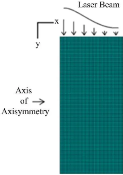
Figure 1: Finite Element Model for laser drilling (Yinzhou et al., 2012).
temperature of each point of the material is obtained through Equation 1. Equation 1 expresses the Fourier's heat transfer within a cylindrical form (Mishra et al., 2013):
, , , , , ,
(1)
where (T) is the temperature-dependent density; C(T) is the temperature-dependent special heat and the K(T) is the temperature-dependent heat transfer coefficient. The mentioned properties for the homogenous materials are constant in all direction, and the used materials in this research are homogenous.
The initial temperature of the model is assumed to be equal to the ambient temperature, T0. So, T(r, z, 0) =T_0. On the t=0, the input energy to the material is equal to the input tempera-ture. According to Equation (1) and by applying the initial conditions, the governing thermal boundary conditions of the mode are presented in equations 2-4. In Equations (2) to (4), is the pulse-on-time and tp is the total pulse time (Mishra et al., 2013).
When 0 < t <τ:
, , , ,
(2)
Whenever τ < t < tp:
, ,
, , (3)
Whenever t > 0:
, ,
, (4)
Each material at a temperature higher than its ambient temperature radiates energy. In the la-ser drilling, the material surface temperature faces severe changes. Therefore, radiation is considered to be a highly significant factor in this process. The heat flux radiated from substance's surface is expressed by the Stefan-Boltzmann law (Akarapu et al., 2004):
q_rad= ∈(Ts^4-T∞^4) (5)
where σ is the constant value of the Boltzmann equal to 5.67×10⁻⁸ , and ∈ is the radiation coeffi-cient equal to 0.9. Furthermore, T_s and T_∞ are the material surface temperature and the am-bient temperature, respectively. On the conducted simulations, the amam-bient temperature is given as 298 ° K.
To consider the losses of the heat as the result of the cooling jet-gas, the convective conductivi-ty was assumed to be 200W/(m^2 k) . The convection heat flux by the Newton Cooling Law is expressed as Equation 6 (Akarapu et al., 2004).
In equation (6), A is the area of the object, h is the heat transfer coefficient, T_s is the material surface temperature and T_∞ is the ambient temperature which is given as 298 °K.
2.2 Simulation Method
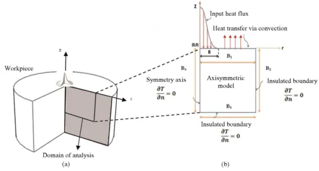
Due to the circularity of the hole sections and also the laser beam, the process modeling can be performed in an axisymmetric form. The most outstanding benefit of axisymmetric modeling is the reduction of the number of elements and, consequently, the reduction of the problem-solving time. Figure 2 illuminates the ideal case in which a laser beam has been modeled as a heat source with Gaussian-distributed heat flux with suitable boundary conditions considering the axisymmetric model of the analysis.
Figure 2: Thermal model of laser drilling process a) Schematic representation of the workpiece. b) Axisymmetric model with boundary condition.
The simulations in this research have been performed through the ABAQUS software. The heat flux load was programmed in FORTRAN as DFLUX subroutine. In order to remove those elements the temperature of which has exceeded the evaporation point, the element death technique has been used.
2.3 Selecting an Appropriate Heat Source Model
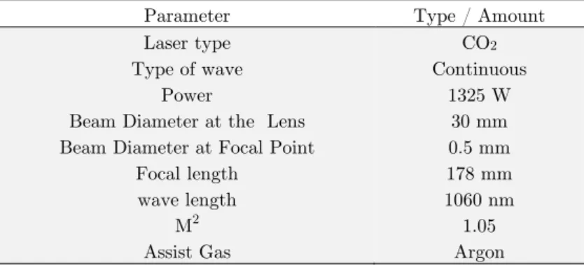
Parameter Type / Amount
Laser type CO2
Type of wave Continuous
Power 1325 W
Beam Diameter at the Lens 30 mm
Beam Diameter at Focal Point 0.5 mm
Focal length 178 mm
wave length 1060 nm
M2 1.05
Assist Gas Argon
Table 1: Laser Parameters used for glass drilling.
In the first type of simulation, the distribution presented in Equation 7 has been used (Yi Zhang et al., 2013).
,
(7)
In Equation 7, P is the laser power, A is the absorption coefficient, ωm is the radius of the laser beam in the focal plane position, ω0 is the radius of the focal point, r is the radial distance from the laser axis, z is the perpendicular distance from the laser focal point, and f is the laser focal distance. Equation 8 has been used for the second type of simulation (Mishra et al., 2013):
4
(8)
In Equation 8, A is the absorption coefficient, P is the laser power, R is the laser effective radi-us, r is the laser beam radiradi-us, L is the laser wavelength, d is the laser beam diameter and f is the laser focal distance.
In simulation type 3, Equation 9 has been used (Yiming Zhang et al., 2014):
q(r) =ηQ/( r_q^2)exp(-r^2/(r_q^2)) (9)
In Equation 9, the value of η is the material absorption coefficient, Q is the laser power, r_q is the laser beam radius, and r is radial distance from the laser beam axis.
The 8-node hexahedral elements, DCAX4, were used for the transient thermal analysis. 5 mi-crometers was chosen as the element optimal length by mesh sensitivity which has been carried out through the trial and error method.
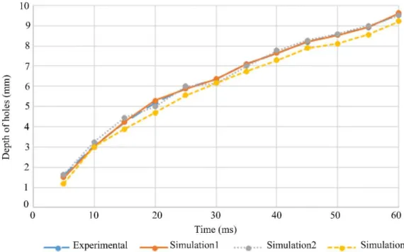
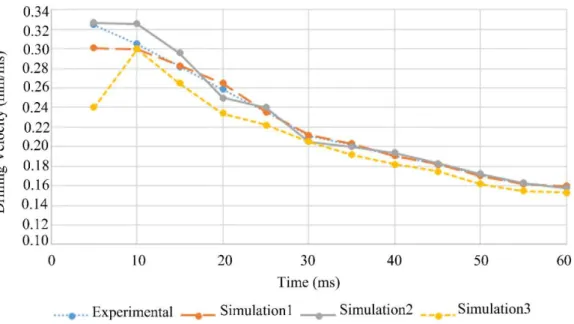
As Table 2, Figures 3 and 4 show, in comparison of the experimental results and the glass laser drilling simulations, the Gaussian distribution No.2, Equation 8, has the best agreement with the experimental results. Therefore, Equation 8 can be used in simulating the drilling process in the next stages.
No Drilling Time
Experimental
results Simulation1 Simulation 2 Simulation 3
Depth (mm)
Velocity (mm/ms)
Depth (mm)
Velocity (mm/ms)
Depth (mm)
Velocity (mm/ms)
Depth (mm)
Velocity (mm/ms)
1 5 1.624 0.324 1.505 0.301 1.635 0.327 1.200 0.240
2 10 3.05 0.305 3.000 0.300 3.255 0.325 3.000 0.300
3 15 4.23 0.282 4.250 0.283 4.445 0.296 3.895 0.265
4 20 5.18 0.259 5.305 0.265 5.000 0.250 4.685 0.234
5 25 5.90 0.236 5.885 0.235 6.005 0.240 5.560 0.222
6 30 6.35 0.211 6.365 0.232 6.155 0.205 6.155 0.205
7 35 7.10 0.202 7.115 0.203 7.000 0.200 6.735 0.192
8 40 7.65 0.191 7.650 0.191 7.775 0.194 7.285 0.182
9 45 8.20 0.182 8.215 0.182 8.275 0.183 7.900 0.175
10 50 8.56 0.171 8.535 0.171 8.600 0.172 8.120 0.162
11 55 8.92 0.162 8.945 0.162 9.005 0.163 8.560 0.155
12 60 9.55 0.159 9.625 0.160 9.490 0.158 9.215 0.153
Table 2: Experimental and Simulated results of glass laser drilling.
Figure 4: Comparison between drilling velocity in experimental and simulated glass laser drilling.
3 EXPERIMENTAL PROCESS AND MODEL VERIFICATION
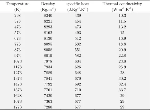
In order to verify the suggested model, Equation 8 presented in section 2.3, three laser drilling ex-perimental tests were performed on the Nickel-base superalloy Inconel 718 with the thickness of one millimeter. The thermo-physical material properties incorporated in the experimental research are presented in Table 3. Fiber laser with the 80- micrometer beam focus diameter was utilized in the experiments.
In the experiments, duty cycle was 50% and the laser focal plane position was equal to 1mm above the workpiece. The overall drilling time in all the three experiments was 0.1 seconds. Figure 5 depicts the experimental process. The experimental conditions are shown in Table 4.
Temperature (K)
Density (Kg.m-3)
specific heat (J.Kg-1.K-1)
Thermal conductivity (W.m-1.K-1)
298 8240 439 10.3
373 8221 454 11.5
473 8293 473 13.2
573 8162 493 15
673 8130 512 16.9
773 8095 532 18.8
873 8058 551 20.9
973 8019 582 22.8
1073 7978 604 23.8
1173 7934 626 25.9
1273 7889 648 28
1373 7841 670 30.2
1473 7792 692 32.4
1573 7761 710 33.7
1628 7420 677 29
1673 7363 677 29
1773 7280 677 29
Table 3: Thermo-physical properties of Inconel 718 used in simulations (Mills 2002).
The geometry features of the entrance and exit hole diameters were measured using Axioskop 40 optical microscope at a magnification of 1000× and the images were exactly measured by the Visilog software. According to Figure 6 and Equation 10, by using the entrance and exit diameters, the value of the taper angle can be achieved.
Figure 6: The Geometry of hole.
Where the (dentrance) is entrance hole diameter, (dexit) is exit hole diameter, and t is the thick-ness of the material.
Simulation procedure in this step is the same as the one presented in Section 2-3. Table 4 shows the different values of hole geometry obtained according to the laser drilling parameters set for the verification experiments along with the amounts of relative verification errors using the simulated approaches.
No
Setting Entrance Diameter Exit Diameter Hole Taper Angle
Laser Power (w) Laser Pulse Frequency (
H
z)
Focal P
lane
Position (mm) Experimental Simulation Error
(%)
Experimental Simulation Error
(%)
Experimental Simulation Error
(%)
1 404 248 1 404 480 -9.09 304 310 -1.97 3.9 4.86 -24.61
2 423 200 1 449 420 6.9 317 300 5.36 3.8 3.43 9.73
3 383 274 1 480 460 4.16 330 320 3.03 3.4 4 -17.64
Table 4: Comparison between simulation and experimental results of Inconel 718.
Low error values yielded by the present model, illustrated in Table4, can guarantee the suitabil-ity and logics of the modeling assumptions in this study. Inaccuracy in measuring the entrance and exit diameters in experimental tests, difference between the theoretical and real values of the exper-imental input parameters such as laser beam radius, laser absorption coefficient and material tem-perature-dependent properties could be the reasons of variation between the software and experi-mental results.
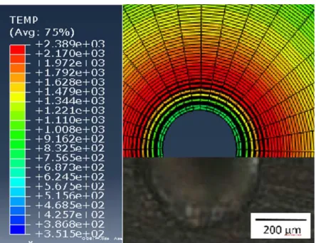
Figure 7 depicts the final shape and temperature distribution of the hole after the simulation process is conducted and element death is performed, while Figure 8 illustrates a comparative image between the experimental and the simulation.
Figure 8: Comparison between simulated and experimental results (Temperature unit is centigrade).
4 EXPERIMENTAL DESIGN AND METHODOLOGY
Response Surface Methodology (RSM) is a set of statistical techniques and applied mathematics to investigate responses (output variables) affected by a number of independent variables (input vari-ables). In each experiment, changes in input variables are made to determine the cause of changes in the response variable (Montgomery 2009). The purpose is to find a relationship between outputs and inputs (responses and parameters) with a minimum error in the form of a mathematical model. Depending on the type of input variable parameters, there are, in general, different ways to design an experiment.
The Response Surface Methodology, RSM, is considered to be a set of mathematical and statis-tical techniques useful for modeling and predicting the desired response (Mahmoud Moradi et al., 2011, Mahmoud Moradi et al., 2014). Also, the RSM specifies the relationships between one or more measured responses and the essential controllable input factors (Mahmoud Moradi et al., 2014).
In the present study, Response Surface Methodology is chosen as the method of design. When all the independent variables are capable of being measured and controlled during an experiment, the response surface is to be expressed as a function through Equation 11.
Y= f(x1, x2, x3,….., xk) (11)
Here, “k” is the number of independent variables. It seems essential to find a rational function to relate the independent variables to the responses. Therefore, a quadratic polynomial function pre-sented in Equation 12 is usually applied in response surface methodology.
In the above equation, β is constant, βi is linear coefficient, βii is coefficient of quadratic, βij is interaction coefficient and ε is the error of the parameters of regression (Mahmoud Moradi et al., 2013). In the present study, after model validation, laser pulse frequency, the duty cycle, the laser power and laser focal plane position were considered to be independent input parameters. Table 5 shows four input variables of the experiment, coded values and actual values of their surfaces. The focal plane position, FPP, was considered as zero when set on upper material surface. Above or below the upper surface, the FPP was considered as positive or negative, respectively. Schematic diagram of FPP is illustrated in Figure 9.
Figure 9: Variation of focal Plane position on the work piece (Ghoreishi et al., 2002).
In the present study, in order to perform the simulation tests, central composite design (CCD), five-level RSM design with four parameters, presented in Table 6, was applied. This plan includes sixteen experiments as factorial points in cubic vertex, eight experiments as axial points and one experiment in the cubic center as center point experiment, meaning a total of 25 experiments have been designed.
The designed experiments have been performed on the Nickel-base superalloy Inconel 718with the thickness of 1mm. Initial temperature of 298 ° K, the convection coefficient of 20W/(m^2 k) and the radiation coefficient equal to 0.9 were considered as the thermal boundary conditions. The interaction time of laser with material is taken to be 0.1 s. The design matrix of the experiments and the obtained results are shown in Table 5.
Variable Sign Unit -2 -1 0 +1 +2
Laser Pulse Frequency F (Hz) 150 250 350 450 550
Laser Power P (W) 200 275 350 425 500
Focal Plane Position FPP (mm) -0.5 -0.25 0 +0.25 +0.5
Duty cycle D (%) 30 40 50 60 70
No
Input Setting Responses
Laser Pulse Frequency Laser Power Focal plane Position Duty cycle Entrance hole diameter (
μ
m)
Exit hole diam
e-ter (
μ
m)
Taper angle Weight of
re-moved mass (mg
× 10
-5 )
1 0 0 0 2 480 230 7.16 84.93
2 2 0 0 0 490 220 7.73 85.22
3 0 0 0 0 400 170 6.58 55.42
4 1 -1 1 -1 410 160 7.16 55.94
5 0 2 0 0 540 260 7.99 107.78
6 1 -1 -1 1 400 150 7.16 52.31
7 1 -1 1 1 440 170 7.73 64.13
8 -1 1 -1 -1 460 200 7.44 74.12
9 -1 -1 -1 1 390 140 6.58 48.82
10 1 1 -1 -1 380 210 4.86 80.96
11 -1 -1 1 1 420 160 7.44 58.07
12 0 0 -2 0 340 120 6.30 36.84
13 -1 1 1 -1 480 200 8.01 79.04
14 -1 1 1 1 490 200 8.30 81.56
15 1 -1 -1 -1 390 150 6.87 50.28
16 -1 -1 1 -1 390 160 6.58 54.87
17 1 1 1 -1 490 210 8.01 83.51
18 -2 0 0 0 320 110 6.01 32.29
19 0 0 2 0 460 200 7.44 74.12
20 -1 -1 -1 1 470 200 7.23 76.56
21 0 0 0 -2 310 90 6.30 28.50
22 1 1 1 1 620 330 8.30 150.55
23 -1 -1 -1 -1 300 120 5.15 30.29
24 1 1 -1 1 500 220 8.01 88.10
25 0 -2 0 0 250 100 4.29 21.03
Table 6: Design Matrix and experimental results.
5 RESULTS AND DISCUSSION
5.1 Entrance Hole Diameter:
In the analysis of variance tables, the P-value expresses the response sensitivity to the input param-eters, and by a decrease in P-value the sensitivity increases. So, in the concept of statistical model-ing, the lower the P-value, the more influential the effect. When the P-value in the analyses of vari-ances is less than 0.05, the term is distinguished as significant (Ghoreishi et al., 2002).
According to the results of analysis of variance on the entrance hole diameter, Table 7, all the main effects of four input parameters; laser power (P), laser pulse frequency (F), duty cycle (D), and the laser focal plane position (FPP) have respectively the highest influences on the diameter of the entrance hole, and all were identified as the effective linear terms. But none of the quadratic and interaction terms were identified as the significant terms. The regression equation obtained is evaluated as significant and Lack-of-Fit as insignificant. In the best analysis, regression is significant and Lack-of-Fit insignificant. Therefore, according to the analysis, the final regression in terms of coded parameter values yields in Equation (13).
Din = 428.80 + 27.92 F + 59.58 P + 24.58 FPP + 27.92 D (13)
An increase in the laser pulse frequency, the laser power and the duty cycle causes an increase in the amount of the thermal flux absorbed by the material and, as a result, it causes an increase in entrance hole diameter. Figures 10 and 11 illustrate response surfaces of entrance hole diameter in terms of input parameters.
Source Degree of
freedom
Adj Sum of squares
Adj Mean
squares T- Value F-Value P-Value
Model 4 137117 34297 ---- 23.85 0.000
Linear 4 137117 34297 ---- 23.85 0.000
Laser pule Frequency 1 18704 18704 3.61 13.01 0.002
Laser Power 1 85204 85204 7.70 59.28 0.000
Focal Plane position 1 14504 14504 3.18 10.09 0.005
duty cycle 1 18704 18704 3.61 13.01 0.002
Error 20 28747 1437
Total 24 165864
R-sq = 82.67 % R-sq (adj) = 79.20 %
Table 7: Revised analysis of variance of entrance hole diameter.
Figure 10: The entrance hole diameter response surface in terms of laser power (P) and laser pulse frequency (F).
Figure 11: The entrance hole diameter response surface in terms of duty cycle (D) and focal plane position (FPP).
5.2 Exit Hole Diameter:
Table 8 shows analysis of variance for the diameter of the exit hole. As shown in Table 8, all main parameters are considered as significant terms and none of the other interaction and quadratic terms are significant. As Table 8 indicates, Lack-of-Fit was determined as insignificant and it shows that a suitable analysis has been performed. Considering the P-Value, laser power, laser pulse fre-quency, laser duty cycle and the laser focal plane position have the highest influence on the exit hole diameter.
According to the performed analysis in ANOVA Table 8, equation 14 represents the regression equation for the exit hole diameter considering significant parameters based on coded values. In the equation (14), which is a linear equation, it should be mentioned that all the main parameters have a positive effect on this response.
Dout = 428.80 + 27.92 F + 59.58 P + 24.58 FPP + 27.92 D (14)
Source Degree of
freedom
Adj Sum of squares
Adj Mean
squares T- Value F-Value P-Value
Model 4 53800 13450.0 ---- 16.83 0.000
Linear 4 53800 13450.0 ---- 16.83 0.000
Laser pule Frequency 1 8067 8066.7 3.18 10.09 0.005
Laser Power 1 32267 32266.7 6.35 40.37 0.000
Focal Plane position 1 5400 5400.0 2.60 6.67 0.017
duty cycle 1 8067 8066.7 3.18 10.09 0.005
Error 20 15984 799.2
Total 24 69784
R-sq = 77.10 % R-sq (adj) = 72.51 %
Table 8: Revised analysis of variance of exit hole diameter.
An increase in the experiment input parameters causes the higher heat absorption at the surface of workpiece, and then the absorbed heat penetrates into the depth of the workpiece resulting in an increase in the lower workpiece surface temperature and consequently causes an increase in the exit hole diameter.
5.3 Hole Taper
Table 9 shows the variance analysis of the hole taper. The only effective parameters are laser power, laser pulse frequency and the focal plane position. Final regression equation of the hole taper re-sponse, based on the significant parameters, is shown in Equation 15 based on coded values.
Taper (˚) = 7.111 + 0.332F + 0.668 P + 0.307 FPP (15)
Consequently, the duty cycle parameter can be defined as an insignificant parameter on the hole taper angle degree, as the statistical analysis confirm it. Figure 12 illustrates the effects of the laser pulse frequency and the laser power on the hole taper angle.
Source Degree of
free-dom
Adj Sum of squares
Adj Mean squares
T- Val-ue
F-Value
P-Value
Model 3 15.617 5.2057 ---- 14.45 0.000
Linear 3 15.617 5.2057 ---- 14.45 0.000
Laser pule
Frequen-cy 1 2.640 2.6401 2.71 7.33 0.013
Laser Power 1 10.720 10.7201 5.46 29.77 0.000
Focal Plane position 1 2.257 2.2571 2.50 6.27 0.021
Error 21 7.563 0.3602
Total 24 23.180
R-sq = 67.37 % R-sq (adj) = 62.71 %
Table 9: Revised analysis of variance of hole taper angle.
Figure 12: The hole taper angle response surface in terms of laser power (P) and laser pulse frequency (F).
As shown in Figure 12, the laser power and the laser pulse frequency having increased, the hole taper angle will increase, the reason of which is the increase in the entrance and exit hole diameters in unequal proportions.
5.4 Weight of Removed Material
influences on the weight of removed material respectively. Therefore, according to the analysis, the final regression in terms of coded parameter values yields in Equation 16:
RM = 66.22 + 9.54 F + 19.72 P + 8.37 FPP + 9.33 D (16)
Source Degree of
freedom
Adj Sum of squares
Adj Mean
squares T- Value F-Value P-Value
Model 4 15282 3820.6 ---- 19.86 0.000
Linear 4 15282 3820.6 ---- 19.86 0.000
Laser pule Frequency 1 2183 2183.3 3.37 11.35 0.008
Laser Power 1 9330 9329.5 6.96 48.49 0.000
Focal Plane position 1 1680 1679.9 3.95 8.73 0.008
duty cycle 1 2090 2089.7 3.30 10.86 0.004
Error 20 3848 192.4
Total 24 19130
R-sq = 77.10 % R-sq (adj) = 72.51 %
Table 10: Revised analysis of weight variance of removed material.
Due to an increase in the input process parameters, the amount of input heat energy absorbed by the workpiece surface increases resulting in melting down more material. Subsequently, the hole dimensions get larger and also the weight of material removed from the hole increases, too.
6 OPTIMIZATION
By statistical analysis of data obtained from simulation tests, regression equations explain logical relations between input variables and responses. The response optimizer option within the DOE module of Minitab 17 statistical software package has been used here to optimize input parametric combinations resulting in the most desirable compromise between different responses using desira-bility function (Saeed Assarzadeh et al., 2015). Table 11 summarizes criterions in order to optimize process parameters. Minimum hole taper and minimum entrance hole diameter are the criteria of the optimization. The reason of not considering the exit hole diameter and the weight of removed material in optimization criteria is that these two responses are dependent on the entrance hole diameter and the extent of taper angle. Whenever the entrance hole diameter and the taper angle are optimized, the exit hole diameter and the weight of removed material will be in an optimized condition, too.
expressed in coded procedure. As it can be seen in Figure 13, all input parameters should be on -2 level, the least value of each parameter, to create an optimized hole.
No Parameter/Response Goal Lower Target Upper Weight Importance
1
Parameters
Frequency Is in range 150 --- 550 --- ---
2 duty cycle Is in range 30 --- 70 --- ---
3 focal plane position Is in range -0.5 --- +0.5 --- ---
4 laser power Is in range 200 --- 500 --- ---
5
Responses D (ent) Minimum 250 250 620 3 3
6 Hole taper Minimum 4.29 4.29 8.3 5 5
Table 11: Constraints and criteria of input parameters and responses.
Figure 13: Calculation of optimal parameters.
Verification simulation was performed at the obtained optimal input parametric setting to com-pare the actual entrance and exit hole diameter and hole taper with those as optimal responses ob-tained from optimization. Table 12 presents the optimization results along with simulation obob-tained responses and their percentage relative verification errors. It is clear that the error percentage of the study is good for engineering applications.
No Optimized Settings
Type of response
Responses
1
Laser pulse frequency (Hz)
Laser power (W)
Duty cycle (%)
Focal plane position (mm)
Entrance hole diameter (μm)
Taper angle
150 200 30 -0.5
Predict 148.8 4.498
Simulation 170 3.436
Error (%) -14.24 23.61
7 CONCLUSIONS
In the present study, the process of laser percussion drilling was simulated using finite element method. The data obtained from the simulated tests were analyzed through DOE. Regarding the performed simulations and statistical analyses, the following conclusions can be drawn:
1.Utilizing all the variable parameters of the laser in Gaussian distribution, such as the wave-length, M2 parameters and the laser focal plane position, is necessary.
2.By an increase in the laser power, the laser pulse frequency, the laser duty cycle and the laser focal plane position, the entrance and exit hole diameters, the hole taper angle and the extent of the weight of material removed from the hole are increased.
3.The laser duty cycle effect on the extent of the hole taper angle was insignificant statistically. 4.By performing optimization process, using desirability approach, the minimum level of each
parameter can be described as the optimum setting of the laser drilling simulation process.
Acknowledgments
The authors would like to thank Malayer University for the financial support of this research.
References
Akarapu, R., Li, B.Q., Segall, A. (2004). A Thermal Stress and Failure Model for Laser Cutting and Forming Opera-tions. journal of Failure Analysis and Prevention . 5 , 51-62.
Dubey, A.K. V. Yadava. (2008). Experimental study of Nd:YAG laser beam machining—An overview. Journal of Materials Processing Technology 195: 15-26.
Ganesh, R.K., A. Faghri, and Y. Hahn. (1997). A generalized thermal modeling for laser drilling process—II. Numer-ical simulation and results. International Journal of Heat and Mass Tranfer 40: 3361-3373.
Ganesh, R.K., A. Faghri, Y. Hahn. (1997). A generalized thermal modeling for laser drilling process—I. Mathemati-cal modeling and numeriMathemati-cal methodology. International Journal of Heat and Mass Transfer. 40, 3351-3360.
Ganguly D, A.B., Kuar. AS,Mitra S. (2012). Hole characteristics optimization in Nd:YAG laser micro-drilling of zirconium oxide by gray relational analysis. Adv Manuf Technol 61: 1255-1262.
Ghoreishi, M. O.B. Nakhjavani. (2008). Optimisation of effective factors in geometrical edifications of laser percus-sion drilled holes. Journal of Materials Processing Technology 196: 303-310.
Ghoreishi, M., D.K.Y. Low, L. Li. (2002). Comparative statistical analysis of hole taper and circularity in laser per-cussion drilling. International Journal of Machine Tools and Manufacture 42: 985-995.
Hanon M.M., E. Akman, B. Genc Oztoprak, M. Gunes, Z.A. Taha, K.I. Hajim, E. Kacar, O. Gundogdu, A. Demir. (2012). Experimental and theoretical investigation of the drilling of alumina ceramic using Nd:YAG pulsed laser. Optics and Laser Technology 44: 913-922.
Jay Tu, Alexander G. Paleocrassas, Nicholas Reeves, Nilesh Rajule. (2014). Experimental characterization of a mi-cro-hole drilling process with short micro-second pulses by a CW single-mode fiber laser. Optics and Lasers in Engi-neering 55: 275-283.
Mahmoud Moradi, M. Ghoreishi, J. Frostevarg, A. F. H. Kaplan. (2013). An investigation on stability of laser hybrid arc welding. Opt. Laser Eng 51: 481-487.
Mahmoud Moradi, Majid Ghoreishi, Mohammad Javad Torkamany. (2014). Modeling and Optimization of Nd:YAG Laser-TIG Hybrid Welding of Stainless Steel. Journal of lasers in Engineering 27: 211-230.
Mahmoud Moradi, Nahid Salimi, Majid Ghoreishi, Hadi Abdollahi, Mahmoud Shamsborhan, Jan Frostevarg, Tor-björn Ilar, Alexander F. H. Kaplan. (2014). Parameter dependencies in laser hybrid arc welding by design of experi-ments and by a mass balance. Journal of Laser Applications 24: 022004-9.
Mills K.C. (2002) Recommended values of thermo physical properties for commercial alloys, Wood head Publishing Limited,Abington ,U.K .
Mishra, S. and V. Yadava, (2013). Modeling and optimization of laser beam percussion drilling of thin aluminum sheet. Optics & Laser Technology 48: 461-474.
Mishra, S. and V. Yadava. (2013). Modeling and optimization of laser beam percussion drilling of nickel-based super-alloy sheet using Nd: YAG laser. Optics and Lasers in Engineering. 51, 681-695.
Montgomery DC. (2009). Design and analysis of experiments, 7th edn, John Wiley, New York.
Parandoush, P. and A. Hossain. (2014). A review of modeling and simulation of laser beam machining. International Journal of Machine Tools and Manufacture 85: 135-145.
Ram K. Ganesh, Wallace W. Bowley, Robert R. Bellantone, Yukap Hahn. (1994). A Model for Laser Hole Drilling in Metals. Journal of Computational Physics 125: 161-176.
Saeed Assarzadeh, Majid Ghoreishi. (2015). Electro-thermal-based finite element simulation and experimental valida-tion of material removal in static gap singlespark die-sinking electro-discharge machining process. J Engineering Manufacture 20: 1-20.
Solana P, K.P., Dowden JM, Marsden PJ. (1998). An analytical model for the laser drilling of metals with absorp-tion within the vapor. Journal of Physics D: Applied Physics 32: 942-952.
Yi Zhang, Shichun Li, Genyu Chen, Jyoti Mazumder. (2013). Experimental observation and simulation of keyhole dynamics during laser drilling. Optics & Laser Technology 48: 405-414.
Yiming Zhang, Zhonghua Shen, Xiaowu Ni. (2014). Modeling and simulation on long pulse laser drilling processing. International Journal of Heat and Mass Transfer 73: 429-437.