Abstract
The nonlinear vibration and normal mode shapes of FG cylindrical shells are investigated using an efficient analytical method. The equations of motion of the shell are based on the Donnell’s non-linear shallow-shell, and the material is assumed to be gradually changed across the thickness according to the simple power law. The solution is provided by first discretizing the equations of mo-tion using the multi-mode Galerkin’s method. The nonlinear nor-mal mode of the system is then extracted using the invariant mani-fold approach and employed to decouple the discretized equations. The homotopy analysis method is finally used to determine the nonlinear frequency. Numerical results are presented for the back-bone curves of FG cylindrical shells, nonlinear mode shapes and also the nonlinear invariant modal surfaces. The volume fraction index and the geometric properties of the shell are found to be effective on the type of nonlinear behavior and also the nonlinear mode shapes of the shell. The circumferential half-wave numbers of the nonlinear mode shapes are found to change with time especially in a thinner cylinder.
Keywords
FG cylindrical shells, Invariant manifold (IM), nonlinear normal mode (NNM), Homotopy analysis method (HAM), nonlinear mode shapes
Nonlinear Vibration and Mode Shapes of FG Cylindrical Shells
1 INTRODUCTION
Functionally graded materials (FGM’s) are the new types of composite materials that have the unique feature of both high thermal and high mechanical properties. The constituent materials of FGMs (usually ceramic and metal) are combined such that the variation of their volume fractions is continuous, giving rise to smooth and gradual change of the mechanical and thermal properties. Hence in spite of the traditional composites that may suffer high amounts of thermal stresses at the interfaces, FGMs could withstand high temperatures while maintaining their structural integrities and providing desirable mechanical properties. These properties makes FGMs a suitable choice for
Saeed Mahmoudkhani a
a Aerospace Engineering Department,
Faculty of New Technologies and Engineering, Shahid Beheshti University, GC, Velenjak Sq., Tehran, Iran, [email protected]
http://dx.doi.org/10.1590/1679-78253270
use in aerospace structures such as outer skins of high speed vehicles, which are commonly in the form of cylindrical shells. The analysis of functionally graded (FG) cylindrical shells is therefore of critical importance and could lead to more efficient structures in the future. Vibration analyses are especially one of the main and critical considerations and thus should be given a high priority in designing cylindrical shell used in aerospace application. Numerous studies have been performed so far on the linear vibration of FG cylindrical shell considering the influence of different parameters such as the edge conditions, temperature rise and follower axial forces (Loy et al. 1999, Pradhan et al. 2000, Haddadpour et al. 2007, Torki et al. 2014). Vibration amplitudes of cylindrical shell may not, however, small enough to be accurately predicted by the linear analysis and thus the geometric nonlinearity should be accounted for. This has been the main concern of many studies in recent years. The work of Mahmoudkhani et al. (2011) is one of the first attempt in this area which is devoted to the analysis of nonlinear primary resonance response of FG cylindrical shells. The multi-mode Galerkin’s procedure together with the method of multiple scales (MMS) is used to obtain the frequency-response curves and identify the ranges of excitation amplitudes and frequencies in which the multi-mode response occurs. The effects of temperature and axial loads on the free and forced nonlinear vibrations of FG cylindrical shells is investigated by Sheng and Wang (2013) and Bich and Xuan Nguyen (2012), using again the Galerkin’s method. Rafiee et al. (2013) investigated the piezoelectric FG cylindrical shell under aerodynamic and thermal loads. Sofiyev (2016) studied the vibration of orthotropic FG cylindrical shells, giving an expression by the Jacobian elliptic function for the nonlinear frequencies. The homotopy perturbation method (HPM) is used to solve the single time equation obtained from the Galerkin’s method. Cylindrical shells with different simply-supported, clamped and free boundary conditions are studied by Strozzi and Pellicano (2013). They used the Chebyshev orthogonal polynomial for discretization of the equations. Jafari et al. (2014) studied the FG cylindrical shell embedded with a piezoelectric layer and used the Multi-mode Ga-lerkin and Runge–Kutta method to provide the solution. More detailed information and references on this subject may be found in the review paper by Alijani and Amabili (2014).
The method of solution adopted in most studies as those mentioned above, begins with discre-tizing the governing partial differential equations (PDEs) with the modal expansion method and then uses either the analytical or numerical methods to determine the periodic response. Among the analytical methods, the MMS is most frequently used due to its established routine. Lower order MMS may not, however, accurate enough as the oscillation amplitude increases. Using higher order MMS may also require heavy mathematical manipulation. Some other analytical methods based on the homogony method such as HPM or Homotopy analysis method (HAM) can give more accurate first order approximation (He 1999, Liao 2003) and their extension to higher orders can be readily performed. Hence they are proper choices for accurate and efficient solution of time equations espe-cially when applied to a single equation. The single time equation obtained by using a single linear mode in the Galerkin’s method is not, however, reliable and may yield erroneous result. Alternative-ly, the nonlinear normal modes (NNM) can be employed to decouple the set of nonlinear equations obtained by the multi-modal Galerkin’s method. The single nonlinear equation that will be obtained in this way, could correctly describe the nonlinear behavior of the system.
performed both on their applications and also their methods of computation (Vakakis 1997, Pierre et al. 2006, Kerschen et al. 2009, Peeters et al. 2009). The invariant manifold (IM) approach, pro-posed by Shaw and Pierre (1993) is one of these methods that defines the NNM as a two-dimensional invariant manifold in phase space. The method extends the invariance property of the linear normal modes to nonlinear systems and may be considered as the generalization of the Ros-enberg’s definition (Peeters 2010). It is to be noted that in contrast to the linear normal modes, the NNMs are not orthogonal, but due to their invariance property they could still be suitable for accu-rate and efficient order reduction in nonlinear oscillatory systems (Kerschen et al. 2009). Moreover the mode shapes corresponding to NNMs would change with amplitude and thus with time (Touze et al. 2004).
IM method is applied in the present study to compute the NNMs of the FG cylindrical shell. For this purpose, the equations of motion, which are based on the Donnell’s shell theory, are first discretized using the multi-mode Galerkin’s method. The obtained ordinary differential equations are then decoupled using the IM method and then solved by HAM to determine the frequency-amplitude relation. Numerical results are obtained for backbone curves and nonlinear invariant surfaces. Nonlinear mode shapes are also presented by depicting the out-of-plane displacement var-iations in axial and circumferential directions.
2 FORMULATION
According to the simple power low, the variation of volume fractions of the ceramic and metal through the thickness direction (z) can be described as,
/ 2 / 2
, 1 ,
N N
m c
z h z h
V V
h h
æ + ö÷ æ + ö÷
ç ÷ ç ÷
=ççç ÷÷ = -ççç ÷÷
è ø è ø (1)
where Vm and Vc represent the volume fractions of metal and ceramic, N is the volume fraction
index and h is the thickness of the shell. The effective material properties of FG shell (Peff)
includ-ing Young’s modulus,E, density, r and Poisson’s ratio, n, are defined as,
, eff m m c c
P =P V +PV (2)
where Pm and Pc denote the material properties of metal and ceramic. Using Eqs. (1) and (2) the effective material properties can be expressed as a function of z,
/ 2
( )( ) .N
eff c m c
z h
P P P P
h - +
= + - (3)
It is evident from Eq. (3) that for N =0, the volume fraction of ceramic become zero and so eff m
P =P i.e. the material composition is pure metal and with the increase in N, the material
2.1 GoverningEquations
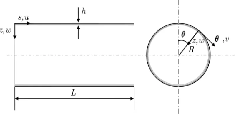
Considering the coordinate system shown in Figure 1 , the equation of motion and the compatibility equation of the FG cylindrical shell can be expressed in terms of redial displacement,w and the airy stress function, Fas (Jansen 2008),
2 11 12 2
1
( ) ( ) F NL( , ) 0,
L w L F L w F
R s
- - - =
¶ (4)
2 21 22 2
1 1
( ) ( ) ( , ) 0,
2 NL
w
L F L w L w w
R s
+ + + =
¶ (5)
Where
4 4 4
11 11 4 12 66 2 2 2 22 4 4
4 4 4
12 21 4 11 22 66 2 2 2 12 4 4
4 4 4
21 22 4 12 66 2 2 2 11 4 4 22 12
2 2 2 2 2 2
() 2( 2 ) ,
() ( 2 ) ,
( ) (2 ) ,
() ( ),
( , ) 2
NL
L D D D D
s R s R
L B B B B B
s R s R
L A A A A
s R s R
L L
T S T
L T S
s R R
q q q q q q q * * * * * * * * * * * * * ¶ ¶ ¶ = + + + ¶ ¶ ¶ ¶ ¶ ¶ ¶ = + + - + ¶ ¶ ¶ ¶ ¶ ¶ ¶ = + + + ¶ ¶ ¶ ¶ = ¶ ¶ ¶ = -¶ 
2 2 2 2 2 2 2 2,
S T S
s qR s q R q s
¶ + ¶ 
¶ ¶ ¶ ¶ ¶ 
(6)
and,
1
A* =A- ,B* =BA-1 ,D* =D-BA B-1 (7)
where A, B and D are the sub-matrices of the stiffness matrix and are defined as,
/2
2 /2
( , , ) (1, , ) ,
h ij ij ij ij
h
A B D Q z z dz
-=
ò
(8)where Qij are the components of the 3´3 stiffness matrix based on the plane-stress Hook’s law whose nonzero components are defined as,
11 22 2 12 2 66
( ) ( ) ( ) ( )
, , .
2(1 ( ))
1 ( ) 1 ( )
E z z E z E z
Q Q Q Q
z z z n n n n = = = = +
- - (9)
It must be noted that to drive the compatibility equation, Eq.(5), the in-plane inertial terms should be neglected and the stress function, F, would be defined in the way to satisfy the in-plane
equations of motion as,
2 2 2
2 2, 2, .
s s
F F F
N N N
R s
R q q s q q
¶ ¶ 
= = =
-¶ -
Figure 1: FG cylindrical shell geometry.
In which Ns and Nq are the normal stress resultant in axial,s, and circumferential directions,
q, respectively. Also, Nsq is the shear stress resultant.
2.2 Discretization of PDEs
The nonlinear PDEs obtained for the equations of motion (i.e., Eqs. (4) and (5)) are first discretized using the Galerkin’s method with appropriate trial functions. Various approximations are used for this purpose in the literatures, among them the function used by (Amabili et al. 1998) contains the minimum number of the linear modal functions needed for accurately predicting the softening be-havior of the shell. This function is defined as,
1 1
11 1 01
1 1
03 1 21
( ) cos( ) sin( ) ( ) sin( ) 3
( ) sin( ) cos(2 ) ( ) sin( ),
m s m s
w W t n W t
L L
m s m s
W t n W t
L L
p p
q
p p
q
= + +
+ (11)
where,W tij( ) ’s are the unknown generalized coordinates to be determined. Substituting the dis-placement function, Eq. (11), into the compatibility equation, Eq. (5), yields a linear non-homogeneous differential equation in F that its particular solution, Fp, can be obtained as,
1
0 1 1 2 1 3 1
1
4 1 5 1 6 1
4 3
1 1
7 1 7 1 11
1 1
1
( ) ( ) cos( ) ( ) cos(2 ) ( ) sin(2 ) sin( )
2 ( ) cos( ) ( ) cos(3 ) ( ) cos(4 ) cos( )
2 2
( ) cos(2 ) sin( ) cos(i ) cos( )
p
i i
i i
i
m s
F f t f t n f t n f t n
L m s
f t n f t n f t n
L
m s im s
f t n f n f
L L
f
p
q q q
p
q q q
p p
q + q +
= =
+
é ù
= +êë + + úû
é + + ù
ê ú
ë û
+ +
+
å
å
2
1 4
1
(2 1)
sin( )
i
i m s
L
p
=
-å
(12)
where f ti( )’s are functions of W tij( )’s. The homogenous solution, Fh, can also be written as,
R
z,w ,v
z,w
s,u h
2 2 2
1 1
,
2 2
h s s
F = N R q + N sq -N R sq q (13)
where Ns, Nq and Nsq are stress resultants that arise from the constraints on the edges of the shell and can be determined in terms of W ti( )’s by applying the average in-plane boundary condi-tions and the continuity requirement of circumferential displacement,
v
(Amabili et al. 1998). The above equation is not a general homogeneous solution and is chosen to satisfy the average in-plane boundary conditions which are defined for the classic simply supported cylindrical shell (i.e., v = 0 and Ns =0) as follows (Amabili et al. 1998),2
2 2
2 2
0 0 0, 0 0 0,
L L
s
F
N Rdsd or R dsd
R
p p
q q
q 
= =
ò ò
ò ò
(14)2
2 2
0 0 0 0 0 0.
L L
s
F
N Rdsd or Rdsd
R s
p p
q q = - ¶¶ ¶q q =
ò ò
ò ò
(15)The continuity of v is also fulfilled via the following relation,
2
0 0 0,
L v
Rdsd
p
q q 
= 
ò ò
(16)where v
q 
¶ can be related to w and Fas,
2 2 2 2
2 21 2 22 2 21 2 22 2
1 ( ) . 2
v F F w w w
A A R B R B w
R
R s s R
q q q q
* * * *
¶ = ¶ + ¶ + ¶ + ¶ + - 
¶ ¶ ¶ ¶ ¶ ¶ (17)
In the above equation F must be replaced by the complete solution of compatibility equation,
i.e., F =Fp+Fh where Fp and Fh are determined by Eqs. (12) and (13). Then using Eq. (11) Ns,
Nq and Nsq can be obtained in terms of the generalized coordinates as,
2 2
1 0 2
22 22
( ) ( ) 0,
8
s s
n W t W t
N N N
R A RA
q q * *
= = = - (18)
Finally, introducing Eqs. (11), (12) and (13) into Eq. (4), and applying the Galerkin’s method, four nonlinear ODEs will be obtained as,
2
2
0 0 0 2
, , 1,3 1 1
, 1,2
( )
( ) ( ) ( ) ( )
( ) ( ) 0, ( , ) (0,1),(0, 3),(1,1),(2,1),
ij
ij ij ijmqs m q s
m q s ijmq m q m q
d W t
W t C W t W t W t
dt
Q W t W t
i j
w
=
=
+ + +
=
=
å
where wijs are linear natural frequencies corresponding to the modes used in Eq. (11) and Cijmqs
and Qijmq are the constants that depend on the material and geometric properties of the cylindrical
shell .
2.3 Extraction of Nonlinear Normal Modes
Eqs. (19) include coupled quadratic and cubic nonlinear terms that may be decupled via the corre-sponding NNMs. To extract the NNMs, the IM approach is used by expressing all the generalized coordinates, W ti( )’s and their time derivatives, W ti( )’s, in terms of W11 and W11. This pair, which
is referred to as the master coordinates, corresponds to the fundamental mode of the shell. Using the definition, u =W11( ),t v =W11( )t , the following fifth order polynomial expansion is used to
ap-proximate the slave coordinates:
1 2 3
(1 ) (2 ) (3 ) ( 1) ( 3) ( 6)
0 0 0
4 5
(4 ) (5 ) ( 10) ( 15)
0 0
1 2 3
(1 ) (2 ) (3 ) ( 1) ( 3) ( 6)
0 0 0
( 10
( )
,
( )
k k k k k k
ij ij k ij k ij k
k k k
k k k k
ij k ij k
k k
k k k k k k
ij ij k ij k ij k
k k k
ij k
W t a u v a u v a u v
a u v a u v
Y t b u v b u v b u v
b - - -+ + + = = = - -+ + = = - - -+ + + = = = + = + + + + = + + +
å
å
å
å
å
å
å
å
4 5
(4 ) (5 ) ) ( 15)
0 0
,
( , ) (0,1),(0, 3),(1,1),(2,1),
k k k k
ij k
k k
u v b u v
i j - -+ = = + =
å
å
(20)where Y tij( )=W tij( ), and aijk and bijk are the unknown constants that could be determined by
sub-stitution of Eq. (20) into the state-space form of the Eqs. (19) and equating the coefficients of like powers of u and v . The final fifth order expressions that will be obtained for W tij( ) are lengthy and may not be given here. But to give an insight to the characteristics of the NNMs, the third order approximation is presented as follows:
2 2
11 2 2
11 11
2 2 2 2
11 11
2 2 3 2 2 2 11 11 11 11 11 2 2 2 2 2 2
11 11 11
(01,03,21)
(2 ) 2
(4 ) (4 )
1 (4 ) 2 (4 ) ( )
,
(9 )( ) (4 )
( , ) (0,1),(0, 3),(2,1).
ij ij ij
ij
ij ij
ij ij ij ij
ij ij mp
mp
S S
W W W
P W P W t W
i j
w w
w w w w
w w w w
w w w w w w
= -= + - -- + -+ - - -=
(21)into Eq. (19), the uncoupled modal ODEs associated with the fundamental NNM of the cylindrical shell can be obtained as follows:
2
11( ) 11 11( ) ( 11, 11) 0,
W t +w W t +G W W = (22)
where,
2 3 2 4
11 11 1 11 2 11 3 11 11 4 11
2 2 4 5
5 11 11 6 11 7 11
3 2 4
8 11 11 9 11 11
( , ) ( ) ( ) ( ) ( )
( ) ( ) ( )
( ) ( ) ( ) ( ) 0,
G W W k W t k W t k W t W t k W
k W t W t k W t k W
k W t W t k W t W t
= + + + +
+ + +
+ =
(23)
with kis being constant terms dependent on the material and geometric properties of the shell.
2.4 Solution by HAM
An efficient and accurate solution can be provided for Eq. (22) using the HAM (Liao 2003). For this purpose, the transformation, t=wNLt and X( )t =W t1( )-d with w and d being the nonlinear
frequency and the constant drift amplitude respectively, are used as follows,
2 2 1
( ) L ( ) [ ( ) , NL ( )] 0.
X X G X X
w t +w t + t +d w t = (24)
The unknown drift is included in the response, since Eq. (22) has quadratic and quartic terms. Considering the initial condition of X(0)=W and X(0)=0, it is reasonable to choose the follow-ing function as an initial guess of the solution,
0( ) cos( ).
X t =W t (25)
The nonlinear operator, Ν is then defined as,
2
2 2
11 2
( ; ) ( ; )
[ ( ; ), ( ), ( )]f tq q q ( )q f tq w f t( ; )q G[ ( ; )f tq ( ), ( )q q f tq ],
t t
¶ 
W D = W + + + D W
¶ 
Ν (26)
where q is the embedding parameter that varies from 0 to 1 and W( )q , D( )q and f t( ; )q are the
functions that represent the solution of the ODE when q=1. The following linear operator is also defined in such a way that it’s homogeneous solution is cos( )t ,
2 2 0 2
( ; )
[ ( ; )]f tq w [ f tq f t( ; )].q t
= +
L (27)
with w0 being the first order approximation of wNL. The zeroth-order deformation equation can
now be defined as,
0 , ( )
where k is the auxiliary undetermined constant parameter that if chosen properly may improve the convergence of the solution. Next, W( )q , D( )q and f( ; )t q are expanded in the Taylor series as,
0
1 0 1
0
1 0 1
0
1 0 1
( ; )
( ; ) ( ; 0) ( ) ( )
! ( ) ( ) (0)
! ( ) ( ) (0)
! m
m m
m m
m q m
m
m m
m m
m q m
m
m m
m m
m q m
t q
t q t q X X q
m q
q
q q q
m q
q
q q q
m q
f
f f t t
w w d d ¥ ¥ = = = ¥ ¥ = = = ¥ ¥ = = = ¶ = + = + ¶ ¶ W
W = W + = +
¶ ¶ D
D = D + = +
å
å
å
å
å
å
(29)
which converges to the exact solutions of wNL, d and X( )t when q=1. That is to say,
0 1 0 1 0 1
( ;1) ( ) ( ) ( ),
(1) , (1) m m NL m m m m
t X X X
f t t t
w w w
d d d
¥ = ¥ = ¥ = = = +
W = = +
D = = +
å
å
å
(30)
where Xm( )t , dm and wm are the unknowns that could be defined via constructing the higher-order
deformation equations by differentiating the zeroth-order deformation equation m times with re-spect to q, then dividing it by m! and finally setting q=0. The resulted m’th order deformation equations is,
m ( 1) 1
[X ( )t -cmXm- ( )]t =k tH( )R Xm[ m-( )]t
L (31)
where cm=0 for m=1 and cm=1 for m >1 and,
1 1 0 [ ( ; ) ( ), ( )] 1 [ ( )] ( 1)! m
m m m
q
t q q q
R X
m q
f
t -
-=
¶ + D W
=
- 
N
(32)
Eq. (32) is a linear differential equation that along with the initial conditions, Xm(0)=0 and
(0) 0
m
X = could be readily solved to obtain higher order approximations of the solution. This is performed along with eliminating the secular terms (i.e., coefficients of cos( )t ), leading to algebraic equations in wm and dm. In numerical analysis of the present problem, it is found that the values of
m
(
)
(
)
4 2 2 11 7 11 2 11 11 0
2 5 3
11 11 8 11 3 11
125 5 6 8
125 250 2
a k a k a
k a k a
w w
w w
- + +
=
+ - (33)
where a11 =W. The first order approximation of the displacement is also obtained as:
(
)
(
)
(
)
(
)
(
)
4 11 2 11 6 4 11 11 2 11 7 11 2 27 8 0 3 0 2 2
0
2 2 2
8 0 7 3 0 2 8 0 7
2 2
0 0
3 9 0
4 3 cos( )
24
125
5 4 cos(3 ) cos(5 )
32 96
32 25
25 sin( ) sin(2 ) sin(4 ) sin(6 )
21 2
125 ( )
4 6 5
125
1 1
6
k k k k
k k k k k
a X a a a k a k a t t t t
t t t t
k
w w
w
k k
w w w
w w
k w
é - - - ù +
ê ú
ë û
é - + - ù +
-ê ú
ë û
é ù
ê- + - + ú
ê ú
ë û
=
(34)
The first order solution presented by Eqs. (33) and (34), is adequately accurate for the range of initial displacement amplitudes considered in the present study. Arbitrarily higher order solutions can however be readily obtained using the mentioned procedure, albeit their corresponding expres-sions are so lengthy to be given here.
3 NUMERICAL RESULTS AND DISCUSSION
Numerical results are presented in this section to examine the accuracy of the IM method used for extraction of NNMs and also the solution of the obtained single nonlinear equation by the HAM. The nonlinear frequency-amplitude of FG cylindrical shells and also the nonlinear mode shapes of the cylindrical shell are also presented and compared with their linear counterparts.
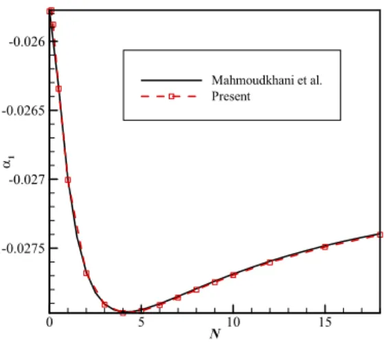
For the verification process it should considered that the solution provided in the present study contains three types of approximation. The first approximation corresponds to the discretization of the partial differential equations (i.e., Eqs. (4) and (5)) which have led to the discretized equations defined by Eq. (19). The second approximation corresponds to the application of the IM approach to Eq. (19), and the third one is related to the analytical solution provided by using the HAM. Therefore, to assess the validity or accuracy of the results obtained by each of these approximations, three numerical studies are performed in Figures 2, 3 and 5. To ensure the validity and convergence of the discretization process used for obtaining Eq. (19), the nonlinearity index, a1 defined in
Mahmoudkhani et al. (2011) by 1 2
11 11 1 1 NL a w a w æ ö÷ ç ÷ ç
= çç - ÷÷ ÷
è ø, is calculated for a cylindrical shell made up of
the stainless steel and the silicon nitride with n1
=
5,
L R/ =2, /h R=0.01,R=0.1m, and different values of N. The results are compared with the result of Mahmoudkhani et al. (2011), as shown inFigure 2: Nonlinearity coefficient, a1, v.s. the volume fraction index, compared with Mahmoudkhani et al. (2011).
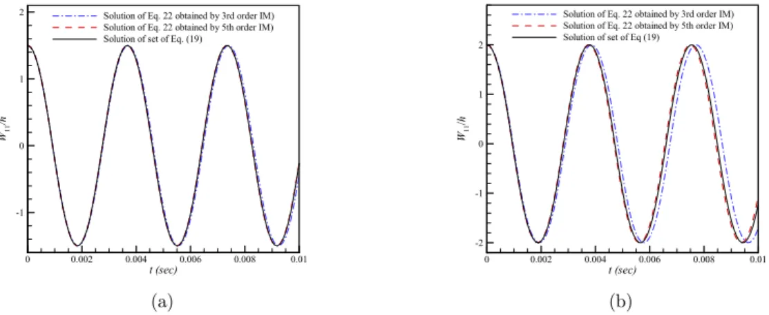
Next the accuracy of the NNM extracted by the IM approach from the discretized equations is examined in Figure 3, by comparing the fundamental nonlinear mode’s response, obtained by the numerical solution of Eq.(22), with the results of numerical simulation of the set of four equations given in Eq. (19). The system parameters used for simulations are
1 10
,
/ 2, / 0.004, 0.5 mn
=
L R = h R = R = . The shell is also assumed to be composed of stainlesssteel and silicon nitride with the material properties given in Table 1. For the initial conditions (ICs), W11(0)=a11 and W11(0)=0 are used and the remaining ICs, required for solution of Eqs. (19),
are obtained using the IM approach to determine Wij(0) (( , )i j ¹(1,1)) in terms of W11 and W11
(i.e., the fifth order version of Eq. (21)). The results, given in Figure 3 match well for a11/h lower
than 1.5 even when the third order IM is used. For higher values of initial displacement, it is seen that the fifth order IM remains accurate when a11/h grows to 2.
Material P0 P-1 P1 P2 P3
Stainless steel
E 201.04e+9 0 3.079e-4 -6.534e-7 0
a 12.330e-6 0 8.086e-4 0 0
n 0.3262 0 -2.002e-4 3.797e-7 0
r 8166 0 0 0 0
Silicon nitride
E 348.43e9 0 -3.07e-4 2.160e-7 -8.946e-11
a 5.8723e-6 0 9.095e-4 0 0
n
0.2400 0 0 0 0r
23700 0 0 0
Table 1: Material properties of FGM’s from Reddy and Chin (1998). N
1
0 5 10 15
-0.0275 -0.027 -0.0265 -0.026
(a) (b)
Figure 3: Comparison of the numerical solution of the single equation obtained by the third and fifth order IM (Eq. (22)) by the numerical solution of set of four equations, Eq. (19), for (a)
11(0) / 1.5
W h = (b)
11(0) / 2
W h = .
The accuracy of the HAM solution is also assessed in Figure 5 by comparing the numerical solu-tion of Eq. (22) with the HAM solusolu-tion. The system parameters are the same as those used in the previous study. To improve the convergence of the solution, the variations of the estimated nonline-ar frequency and also the response amplitude at an nonline-arbitrnonline-ary time instant with k are depicted first in Figure 4 Different-order HAM approximations are included in this figure. The best accuracy may be obtained by choosing k from the region where the variation of the solution with k is minimal. Hence k= -1 might be proper choice for the analysis. Time histories obtained by different order HAM for a11/h=2 is compared in Figure 5-(a) with the numerical solution. Excellent agreement is seen in Figure 5-(a) with even first order HAM. To emphasize on the accuracy of the HAM for higher initial displacement, results obtained for a11/h=6 are also given in Figure 5-(b), which shows that the fourth-order HAM have completely matched with the numerical result.
Figure 4: Variation of the frequency ratio and the response amplitude at
time t0 =0.004 sec with the auxiliary parameter k.
The HAM, then is used to calculate the nonlinear backbone curves of the cylindrical shell with
t (sec) W11
/h
0 0.002 0.004 0.006 0.008 0.01
-1 0 1
2 Solution of Eq. 22 obtained by 3rd order IM)
Solution of Eq. 22 obtained by 5th order IM) Solution of set of Eq. (19)
t (sec) W11
/
h
0 0.002 0.004 0.006 0.008 0.01
-2 -1 0 1 2
Solution of Eq. 22 obtained by 3rd order IM) Solution of Eq. 22 obtained by 5th order IM) Solution of set of Eq (19)
NL
/
L
W11 (t0
)/
h
-4 -2 0 2
0.85 0.9 0.95 1
1.99956 1.99975 1.99994
NL/L(4th order HAM) W11(t0)/h (4th order HAM) NL/L(3rd order HAM) W
dex, N . The variation of the nonlinear frequencies (wNL) with nondimensional amplitude (a11/h)
is given in Figure 6-(a). As N increases it is seen that the corresponding frequencies increase due to
higher contribution of the ceramic part in the FGM. All the curves also show the softening behavior. To better illustrate the effect of N on the strength of the softening nonlinearity,
11
/
NL
w w v.s.
11/
a h is depicted in Figure 6-(b). The slight increase in the bending of the curves is greater for
intermediate values of N (N =1, 5). Similar study is also performed in Figure 7 for other system parameters taken as, n1
=
8,
L R/ =2, /h R=0.001,R=1m. The nonlinearity is mostly hardening in this case, which is completely different from the previous one. The curves obtained in Figure 7-(b), also show the considerable effect of N on the nonlinearity. As is evident, for some intermediatevalues of N (N =5,10), wNL/w11 initially decrease with amplitude and then, after a certain am-plitude, begins to rise. For other values of N , the most strong nonlinearity (i.e., bending of the
backbone curve) occurs for N = 0which decreases as Ngrows.
(a) (b)
Figure 5: Displacement time history of the fundamental NNM amplitude obtained by the numerical method and HAM for (a)
11(0) / 3
W h = (b)
11(0) / 6
W h = .
(a) (b)
Figure 6: (a) Amplitude v.s. wNL (b) Amplitude v.s. wNL /w11. Corresponding to the fundamental NNM with n1
=
10,
L/R=2, R= 0.5 m,h/R =0.004.t (sec) W11
/h
0 0.002 0.004 0.006 0.008 0.01
-3 -2 -1 0 1 2 3
Numerical solution 1st order HAM
t (sec) W11
/
h
0 0.002 0.004
-6 -3 0 3 6
Numerical solution 1st order HAM 4th order HAM
NL a11
/
h
1400 1600 1800 2000 2200 2400 2600
0.5 1 1.5
N=0 N=1 N=5 N=10 N=15 N=20
NL/11
a11
/
h
0.985 0.99 0.995 1
0.5 1 1.5 2
(a) (b)
Figure 7: (a) Amplitude v.s. wNL (b) Amplitude v.s.
11
/
NL
w w . Corresponding to the
fundamental NNM with n1
=
8,
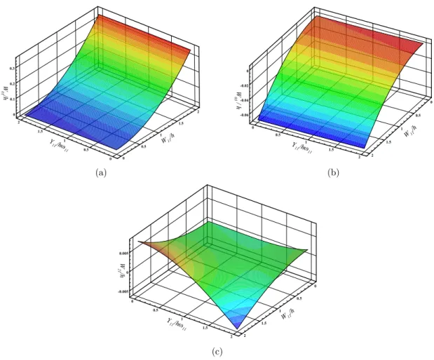
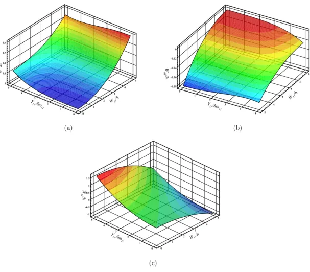
L/R =2, R=1 m,h/R =0.001.The invariant nonlinear modal surfaces corresponding to the fundamental NNM of the shell are next obtained in Figures 8 and 9, for the two cases of the cylindrical shells studied above. These surfaces depict the variation of the linear modal amplitudes, W01, W03 and W21 with W11 and W11.
The results presented in Figure 8 for the first case study, show that W01 and W03 have a small dependence on W11 although they considerably varies with W11. It is in contrast with W21, which has comparable dependency on both W11 and W11. However, the contribution of the mode
associat-ed with W21 to the NNM is not considerable as the magnitude of W21 is much smaller than the magnitudes of W01 and W03. This implies that the axisymmetric modes are mainly responsible for the softening behavior observed in Figure 6.
The invariant surfaces of the second case study are shown in Figure 9. Comparing with the re-sult of Figure 8, W11 is seen to have more influence, in this case, on W01 and W03, although the
effect of W11 is still dominant. Moreover, W21 has the greatest amplitude and thus the
correspond-ing mode is the most dominant mode in the NNM compared to the axisymmetric modes. This mode is, therefore, the main cause of the hardening type nonlinearity seen in Figure 7. Also, due to the considerable effect of W11 on W21, and also considering that W11 and W21 correspond to the modes with one longitudinal half wave number and different circumferential wave numbers, it may be inferred that the nonlinear mode shape may significantly vary with time along the circumferential direction. This is examined in the next numerical studies in Figures 10 and 11. In these figures, the nonlinear mode shapes of the cylindrical shell is compared with their linear counterparts.
NL
a11
/
h
250 300 350 400 450
0.5 1 1.5 2 2.5 3 3.5 4
N=0 N=1 N=5 N=10 N=15 N=20
NL/11
a11
/
h
1 1.002 1.004 1.006 1.008 1.01 1.012 0.5
1 1.5 2 2.5 3 3.5
(a) (b)
(c)
Figure 8: The nonlinear invariant modal surface obtained for fundamental NNM by fifth order IM (a)W01
/
h (b) W03/
h (c) W21/
h v.s. W11/
h and W11/
w
NLh for1 10
,
1,
/ 2, / 0.004, 0.5 mn
=
N = L R = h R= R = .As is previously mentioned, the nonlinear mode shapes may not remain the same at different instants. Hence the mode shapes in Figures 10 and 11 are presented for three different time instants. Moreover at each time instants, the displacement distributions in longitudinal and circumferential directions are given in the same two dimensional plot. For the longitudinal distribution, q is set to zero and for the circumferential direction, s is set to L/ 2. The linear mode shapes are also includ-ed in these figures to illustrate the effects of the nonlinearity on the mode shapes. Results in Figure 10 correspond to the first case study, whose corresponding invariant surfaces are presented in Fig-ure 8. The mode shapes at t=0 where W11 is zero, are shown in Figure 10-(a). Slight differences between the linear and nonlinear mode shapes, both for longitudinal and circumferential directions, can be recognized, although the overall shapes are the same. Mode shapes at t =0.25TNL where
2 /
NL NL
T = p w is depicted in Figure 10-(b). The displacement amplitude (W11) is nearly zero at this W11/h
0 0.5
1 1.5
2
Y 11/h
11
0 0.5 1 1.5 2
W
0
1/h
0 0.1 0.2 0.3
W11/h
0
0.5
1
1.5
2
Y 11/h
11
0 0.5
1 1.5
2
W
03
/h
-0.06 -0.04 -0.02 0
W11/h
0
0.5
1
1.5
2
Y 11/h
11
0 0.5
1 1.5
2
W
21
/h
point, while W11 is close to its maximum value. The nonlinear mode’s displacement distribution in both longitudinal and circumferential direction deviate considerably from their linear counterparts such that the number of circumferential half-wave numbers are doubled at this instant. This hap-pens due to the fact that the amplitude of W21, which corresponds to the mode with 2n1 circumfer-ential half-wave number, becomes dominant at this time. However, since W21 have much lower am-plitudes in most times than the modes with n1 circumferential half-wave numbers (see Figure 8), thus the nonlinear mode shape seen in Figure 10-(b) can be observed only in a small interval of time. The mode shapes at t =0.5TNL are also similar to those at t=0, especially in the
circumfer-ential direction.
(a) (b)
(c)
Figure 9: The nonlinear invariant modal surface obtained for fundamental NNM by fifth order IM
01
/
W h (b)
03
/
W h (c)
21
/
W h v.s.
11
/
W h and
11
/
NLW
w
h for= = = =
=
1 8
,
1,
/ 2, / 0.001, 1 m,n N L R h R R
W11/h
0 1
2 3
4 5
Y 11/h
11
0 1 2 3 4 5
W
01
/h
0 0.1 0.2 0.3 0.4
W11/h
0
1
2
3
4
5
Y 11/h
11
0 1
2 3
4 5
W
03
/h
-0.08 -0.06 -0.04 -0.02 0
W11/h
0 1
2 3
4 5
Y
11/h 11
0 1 2 3 4 5
W
21
/h
(a) t = 0 (b) t = 0.25T
NL (c) t = 0.5TNL
Figure 10: Fundamental nonlinear mode shape of the cylindrical shell in different instants for
= = = =
=
1 10
,
1, / 2, / 0.004, 0.5 m,n N L R h R R
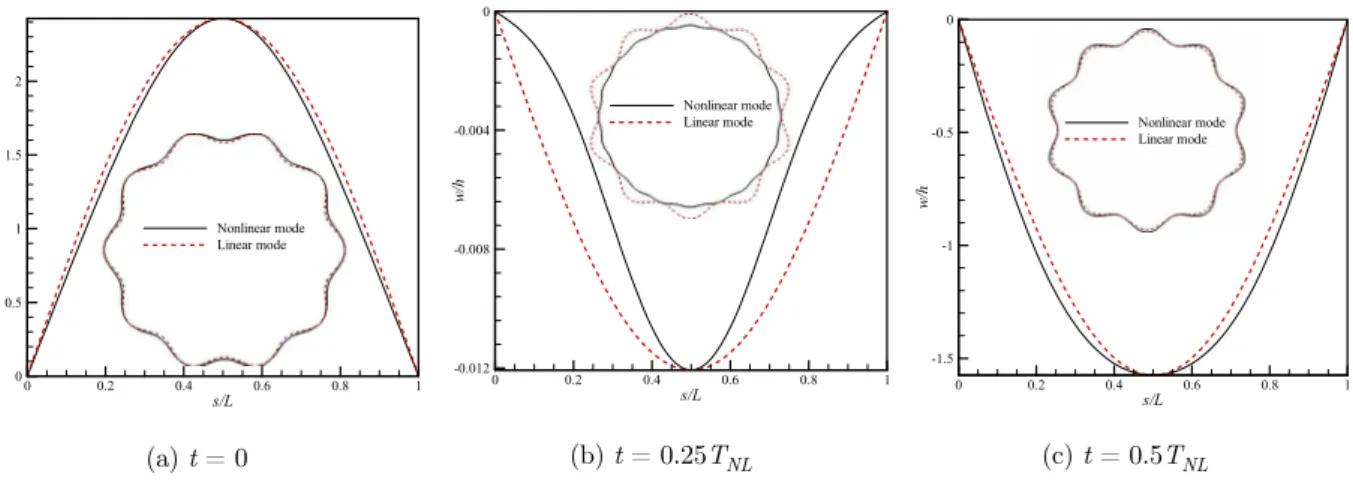
Mode shapes of the second case study, shown in Figure 11, exhibits a rather different nonlinear mode shapes in comparison to the first case. The displacement distribution in the longitudinal di-rection is nearly the same as the linear mode shapes, at different instants of time. However, the distributions in the circumferential direction are very different from the linear modes, such that at
0
t= and 0.5TNL the mode shapes are similar to the trapezoidal form rather than the sinusoidal form. This is in fact due to larger amplitudes of W21 as is seen in Figure 9. Moreover, the
circumfer-ential wave numbers at t =0.25TNL (where the velocity has its maximum value), is twice the wave number of the linear mode shape. This is similar to what is observed for the first case in Figure 10-(b), except that the mode’s maximum amplitude is much larger in this case and the nonlinear mode shape with 2n1 circumferential half-wave number is much more pronounced.
(a) at t = 0 (b) at t = 0.25TNL (c)at t = 0.5TNL
Figure 11: Fundamental nonlinear mode shape of the cylindrical shell in different
instants for
1 8
,
1, / 2, / 0.001, 1 mn
=
N = L R = h R = R = .s/L
w
/h
0 0.2 0.4 0.6 0.8 1
0 0.5 1 1.5 2
Nonlinear mode Linear mode
s/L
w/
h
0 0.2 0.4 0.6 0.8 1
-0.012 -0.008 -0.004 0
Nonlinear mode Linear mode
s/L
w/
h
0 0.2 0.4 0.6 0.8 1
-1.5 -1 -0.5 0
Nonlinear mode Linear mode
s/L
w/
h
0 0.2 0.4 0.6 0.8 1
0 0.5 1 1.5 2 2.5 3 3.5 4
Nonlinear mode Linear mode
s/L
w/
h
0 0.2 0.4 0.6 0.8 1
0 0.5 1 1.5
Nonlinear mode Linear mode
s/L
w/
h
0 0.2 0.4 0.6 0.8 1
-5 -4 -3 -2 -1 0
4 CONCLUSIONS
The nonlinear mode shapes of the FG cylindrical shell was calculated using the fifth-order IM ap-proach and was employed along with the HAM to provide an expression for the frequency-amplitude relation of FG cylindrical shells. For this purpose, the governing PDEs were discretized using the most influential linear modes of the structure. These equations were then decoupled using the NNM, leading to a single nonlinear ordinary equation for the fundamental mode. The HAM was applied to solve this equation which was shown to give an accurate result even with the first ap-proximation, in the reasonable range of displacement amplitudes considered in the present study.
Numerical studies were performed to examine the accuracy of the IM and HAM. Moreover the backbone curves, the nonlinear invariant surfaces and also the nonlinear mode shapes of the FG cylindrical shell were obtained for two different thickness to radius ratios. The softening nonlineari-ty with minimal dependence on N was observed for the thicker shell. The thinner cylinder,
howev-er, exhibited the hardening behavior with the most nonlinearity occurred for lower values of N. It
was found that the axisymmetric mode with twice circumferential wave number (i.e., mode (2,1)) is the dominant mode, compared to the axisymmetric modes, that contributes to the NNM in the thinner cylinder. Moreover, the dependence of (2,1) mode’s amplitude on both the displacement and velocity of the mode (1,1) was found to be comparable, in contrast to the axisymmetric modes that were mostly dependent on the displacement. Hence in times that the displacement and velocity of the (1,1) mode reach their zero and maximum values, respectively, the amplitude of the mode (2,1) becomes dominant leading to the nonlinear mode shapes with circumferential wave number twice those observed for the linear mode shapes. This was in fact more pronounced for the thinner cylin-der.
References
Alijani, F., Amabili, M., (2014). Non-linear vibrations of shells: A literature review from 2003 to 2013. International Journal of Non-Linear Mechanics 58:233-257.
Amabili, M., Pellicano, F., PaÏDoussis, M.P., (1998). Nonlinear vibrations of simply supported, circular cylindrical shells, coupled to quiescent fluid. Journal of Fluids and Structures 12(7):883-918.
Bich, D.H., Xuan Nguyen, N., (2012). Nonlinear vibration of functionally graded circular cylindrical shells based on improved Donnell equations. Journal of Sound and Vibration 331(25):5488-5501.
Haddadpour, H., Mahmoudkhani, S., Navazi, H.M., (2007). Free vibration analysis of functionally graded cylindrical shells including thermal effects. Thin-Walled Structures 45(6):591-599.
He, J.-H., (1999). Homotopy perturbation technique. Computer Methods in Applied Mechanics and Engineering 178(3–4): 257-262.
Jafari, A.A., Khalili, S.M.R., Tavakolian, M., (2014). Nonlinear vibration of functionally graded cylindrical shells embedded with a piezoelectric layer. Thin-Walled Structures 79:8-15.
Jansen, E.L., (2008). A perturbation method for nonlinear vibrations of imperfect structures: Application to cylindri-cal shell vibrations. International Journal of Solids and Structures 45(3–4):1124-1145.
Kerschen, G., Peeters, M., Golinval, J.C., Vakakis, A.F., (2009). Nonlinear normal modes, Part I: A useful frame-work for the structural dynamicist. Mechanical Systems and Signal Processing 23(1):170-194.
Loy, C.T., Lam, K.Y., Reddy, J.N., (1999). Vibration of functionally graded cylindrical shells. International Journal of Mechanical Sciences 41(3):309-324.
Mahmoudkhani, S., Navazi, H.M., Haddadpour, H., (2011). An analytical study of the non-linear vibrations of cylin-drical shells. International Journal of Non-Linear Mechanics 46(10):1361-1372.
Nayfeh, A.H., Nayfeh, S.A., (1995). Nonlinear normal modes of a continuous system with quadratic nonlinearities. Journal of Vibration and Acoustics 117(2):199-205.
Peeters, M. (2010). Theoretical and Experimental Modal Analysis of Nonlinear Vibrating Structures using Nonlinear Normal Modes, Ph.D. Thesis, University of Liège.
Peeters, M., Viguié, R., Sérandour, G., Kerschen, G., Golinval, J.C., (2009). Nonlinear normal modes, Part II: To-ward a practical computation using numerical continuation techniques. Mechanical Systems and Signal Processing 23(1):195-216.
Pierre, C., Jiang, D., Shaw, S., (2006). Nonlinear normal modes and their application in structural dynamics. Math-ematical Problems in Engineering.
Pradhan, S.C., Loy, C.T., Lam, K.Y., Reddy, J.N., (2000). Vibration characteristics of functionally graded cylindri-cal shells under various boundary conditions. Applied Acoustics 61(1):111-129.
Rafiee, M., Mohammadi, M., Sobhani Aragh, B., Yaghoobi, H., (2013). Nonlinear free and forced thermo-electro-aero-elastic vibration and dynamic response of piezoelectric functionally graded laminated composite shells: Part II: Numerical results. Composite Structures 103:188-196.
Reddy, J.N., Chin, C.D., (1998). Thermomechanical analysis of functionally graded cylinders and plates. Journal of Thermal Stresses 21(6):593-626.
Rosenberg, R.M., (1962). The Normal Modes of Nonlinear n-Degree-of-Freedom Systems. Journal of Applied Me-chanics 29(1):7-14.
Shaw, S.W., Pierre, C., (1993). Normal Modes for Non-Linear Vibratory Systems. Journal of Sound and Vibration 164(1):85-124.
Sheng, G.G., Wang, X., (2013). An analytical study of the non-linear vibrations of functionally graded cylindrical shells subjected to thermal and axial loads. Composite Structures 97:261-268.
Sofiyev, A.H., (2016). Nonlinear free vibration of shear deformable orthotropic functionally graded cylindrical shells. Composite Structures 142:35-44.
Strozzi, M., Pellicano, F., (2013). Nonlinear vibrations of functionally graded cylindrical shells. Thin-Walled Struc-tures 67: 63-77.
Torki, M.E., Kazemi, M.T., Haddadpour, H., Mahmoudkhani, S., (2014). Dynamic stability of cantilevered function-ally graded cylindrical shells under axial follower forces. Thin-Walled Structures 79:138-146.
Touze´, C., Thomas, O., Huberdeau, A., (2004). Asymptotic non-linear normal modes for large-amplitude vibrations of continuous structures. Computers and Structures 82:2671-2682.