Lat. Am. j. solids struct. vol.14 número5

Abstract

Aiming at multiscale numerical investigations of fibrous connective tissues, the present work proposes a finite strain viscoelastic model suitable to represent the local mechanical response of living cells in conjunction with finite element simulations of nanoindentation tests. The material model is formulated in a thermodynamically consistent framework based on a variational constitutive approach. As a case of study, a numerical investigation of the local compress-ible response of fibroblast cells is addressed. Moreover, a set of cyclic, stress relaxation and creep experiments are simulated in order to investigate the capability of the model to predict rate dependence of cells, showing sound agreement with experimental data. The proposed model may be used as a suitable tool for a better understanding of stiffness and energetic dissipation of cells.

Keywords

Living cells, Viscoelasticity, Constitutive model, AFM nanoinden-tation, Multiscale.

Modeling the Local Viscoelastic Behavior of Living

Cells Under Nanoindentation Tests

1 INTRODUCTION

Withstanding mechanical loadings is the primary function of many biological connective tissues such as tendons, ligaments and cartilage. The mechanical response to external loadings are highly dependent on their hierarchical microstructure, cellular organization and interactions between one another (Lavagnino et al., 2015).

On its hierarchy inside the tissue, cells are subjected to a complex mechanical environment (Qi et al., 2006). These mechanical stimuli are transduced by cells into biochemical signals leading to tissue adaptation. The particular mechano-chemical pathways that induce changes in tissue

mor-Thiago André Carniel a Eduardo Alberto Fancello a,b,*

a _{GRANTE - Department of Mechanical}

Engineering, Universidade Federal de Santa Catarina, Florianópolis, SC, Brazil. carnielta@gmail.com

b _{LEBm - University Hospital,}

Universi-dade Federal de Santa Catarina, Floria-nópolis, SC, Brazil.

eduardo.fancello@ufsc.br

* Corresponding author

http://dx.doi.org/10.1590/1679-78253748

phology are usually known as mechanotransduction mechanisms (Lavagnino et al., 2015; Wang, 2006).

Regardless their physiological functions, living cells are structural units holding particular non-linear behaviors, including viscous and plastic effects (Bonakdar et al., 2016; Haase and Pelling, 2015; Nawaz et al., 2012). Accordingly, cells may present important mechanical contributions in the macroscopic response of tissues, where multiscale analysis can be employed to investigate these mi-cromechanical behaviors.

In multiscale numerical analyses based on representative volume elements (RVE), the homoge-nized behavior relies strongly on how accurate the behavior of each material phase is represented by corresponding specific material models. In addition, these models must show sound agreement with experimental data at that scale, specifically in cases where these phases present nonlinear behavior and are subjected to finite strains.

Several measurement techniques have been employed to assess the mechanical response of living cells, such as micropipette aspiration, magnetic and optical tweezers and atomic force microscopy (AFM) indentation, also known as nanoindentation test (Haase and Pelling, 2015; Janmey and McCulloch, 2007; Kollmannsberger and Fabry, 2011). Among these experimental methods, the later provides a convenient structure to finite element simulations. For instance, whereas the cell sample can be considered locally as a homogenous medium, the tip of the indenter is modeled as a rigid body.

With these motivations in mind and aiming future numerical multiscale investigations of fibrous soft tissues, the present work proposes a finite strain viscoelastic model suitable to represent the local mechanical response of living cells in conjunction with finite element simulations of nanoinden-tation tests. The proposed model is formulated in a thermodynamically consistent framework based on the variational formalism addressed in Ortiz and Stainier (1999) and Radovitzky and Ortiz (1999), particularized in Fancello et al. (2006) and Vassoler et al. (2012) to viscoelastic materials. In addition, an alternative incremental solution strategy is proposed.

This manuscript is organized as follows. Section 2 presents the theoretical background employed to model the viscoelastic behavior of cells. Aiming finite element simulations, the continuum consti-tutive equations are discretized in time, leading to a variational consticonsti-tutive update algorithm, shown in section 3. In order to verify if the material model is able to represent the available experi-mental data, section 4 addresses a set of numerical simulations of nanoindentation experiments of fibroblast cells. In addition, the compressible and viscoelastic responses of the model are studied. Particularities of the finite element simulations and further discussions about the mechanical behav-ior of cells are highlighted in section 5. Finally, appendices provide operational details and the ana-lytical expression for the consistent material tangent modulus.

2 CONTINUUM FORMULATION

2.1 Constitutive Modeling of Dissipative Materials in a Variational Framework

and Bazant, 2002). The argument of the free energy, in the case of an isothermal process, is the thermodynamic state defined by the deformation gradient F and a set of internal variables a. The

dissipation potential ¡, on the other hand, depends also on the corresponding rates F and a , where the semicolon in the argument list indicates the state variables play a role of parameters. For the sake of clarity, only the dependence on the rates is kept henceforward in the notation of this potential.

It is hypothesized that a =a

(

)

(

)

( )

( )

¡ F,a :=j F +f a . _(2.1)

Based on these assumptions, it is shown in Ortiz and Stainier (1999) and Radovitzky and Ortiz (1999) that a potential  of the form

(

)

(

)

(

)

(

)

(

)

¶ ¶

F F

F F F F

F

a a

a a a a

a

 _   _  _   _

 (2.2)

may be defined such that the optimality condition of the minimization problem

(

)

arg inf ,

= F

a

a a

 

   _(2.3)

provides a thermodynamically consistent equation for the evolution of the internal variables:

(

)

( )

y f

¶ ¶

+ =

¶ ¶

F

0

a a

a a



 . (2.4)

The first Piola-Kirchhoff stress tensor is computed from the first partial derivative of the rate potential with respect to F . Moreover, the rate potential evaluated at the minimizer argument of (2.2) defines a reduced potential _red_{, whose total derivative with respect to} F also results in the first Piola-Kirchhoff stress tensor:

(

)

( )

_{( )}

₍

₎

red

red

, d

, : inf ,

d where

j

y ¶

¶ ¶

= = = + =

¶

¶ ¶

F F

P F F

F

F F F a

a

a 



 _{ }

  

 

  . (2.5)

Potential _red _{plays an important role in present framework, since its incremental counterpart}

presents a compelling mathematical structure for the calculation of the incremental updates of the internal variables.

2.2 Thermodynamic Potentials for a Class of Viscoelastic Models

The classic multiplicative decomposition of the deformation gradient F is used herein to separate

elastic _Fe _{and viscous F}v _{contributions:}

( )

( )

e v_{, J}e _{: det} e _{0, J}v _{: det} v ₀

= = > = >

F F F F F . _(2.6)

T _{e e}T _{e v v}T _v

:= , := , :=

C F F C F F C F F _. (2.7)

Similarly, total and viscous rate of deformations are formally defined as

( )

( )

( )

1

1

v v v v v v

: sym , ,

: sym , skew ,

-= =

= = = =

d l l FF

d l l F F l 0



 (2.8)

where the assumption of null inelastic spin is used (Anand and Gurtin, 2003; Gurtin and Anand, 2005).

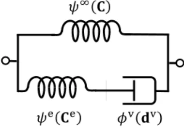
The proposed model follows the rheological assembly illustrated in Figure 1. According to this, the set of internal variables is reduced to _a:=

{ }

potential take the form:

( )

( )

( )

: , :

y ₌ y¥ _{C +}y _C f ₌ f _{d .}

(2.9)

The superscript ¥ represents the time-independent response. As can be noted, the dissipation potential j of equation (2.1) is null. Moreover, the arguments of the potentials (2.9) are objective entities (Gurtin et al., 2010).

Figure 1: Schematic representation of the rheological model.

In view of (2.9), the rate potential (2.2) reduces to the expression:

(

)

(

)

( )

 _(2.10)

with _dv _{depending on F}v _{by means of (2.8). Equation (2.10) provides a continuum background for}

the variational approach introduced in section 2.1. The incremental counterpart of the constitutive equations and numerical issues are addressed in the next section.

3 INCREMENTAL FORMULATION

3.1 Incremental Potential and Updating Rule for the Internal Variable

An incremental counterpart of the rate potential (2.10) is used to directly compute the incremental internal variable updates needed in finite element schemes. Considering a time increment

1

n n

t t ₊ t

(

)

(

)

(

)

( )

v v v v v

inc n , n : n , n n, n

n

t

t

J

y y f

+ + + +

+

é ù

= - _{+ D êë úû}

F F F F F F d

 , _(3.1)

where the variables _dv

( )

note that _fv _{is evaluated at an intermediate time}

n

t _+J inside the time increment, where the

param-eter JÎ ë ûé0,1ù is closely related to the discretization rule employed for _Fv_{. The consistency of the}

incremental form (3.1) can be verified if D  t 0 _inc =.

The most common option to obtain an update expression for the internal variable 1

v

n+

F , in

func-tion of the discrete tensor _dv_{, is the well-known exponential mapping (Weber and Anand, 1990):}

(

)

1 1

v v 1 _ln v v v _exp( v₎ v

n n n t n

t

-+ +

» = = D

D 

d d F F F d F . _(3.2)

This choice has been extensively used in combination with the spectral parameterization of _dv

to handle arbitrary isotropic hyperelastic potentials or in combination with Hencky’s isotropic mod-el to obtain some numerical advantages (Fancmod-ello et al., 2006; Fancmod-ello et al., 2008; Vassoler et al., 2012). Moreover, under an incompressible viscous flow assumption, the incremental relation

( )

tr d = 0 

( )

1

v

det Fn+ =1 is automatically fulfilled.

Another alternative expression to obtain the updated value 1

v

n+

F is based on the classical Euler

integration rule:

(

)

1

1

v v v v _, v ₁ v v

n J n J J n J n

-+ + +

» = = - +

d d F F F F F , _(3.3)

(

)

v v 1 v

n n

t +

-D

» =

F F F F . _(3.4)

When J=1, a fully implicit integration scheme is recovered. In this case, substituting equation (3.4) into (3.3) leads to the following updating rule:

(

)

1

1

v v v

n+ t n

-= - D

F I d F , (3.5)

where I is the second order identity tensor.

In view of the parameterization (3.5), the resulting variational problem is formulated in a fully tensorial format. While this implies the simultaneous evaluation of a set of independent compo-nents, the formulation remains able to handle anisotropic behaviors. Moreover, neither the spectral decomposition of _dv_{, nor the first and second derivatives of these spectral quantities are needed. In}

addition, if the viscous flow is considered incompressible, it is enforced into the variational problem by means of a Lagrangian functional (further details in next section).

3.2 Constitutive Algorithm

The local constitutive algorithm is composed by two main stages: the solution of the variational principle and the stress evaluation. Accordingly, the general concepts introduced in section 2 are particularized to the present class of viscoelastic models.

3.2.1 Solution of the Variational Principle

In view of the parameterization (3.5), the viscous rate of deformation becomes the primal variable of the variational problem. Moreover, in the present modeling, the viscous flow is considered incom-pressible. Therefore, the minimum principle (2.3) can be presented as

opt

v ₁

v

inc cte

arg inf

n

so += Î

=

F d

d _

  , (3.6)

where

{

( )

}

v _det v v ₁

n

so d Î ym éê_ëF+ d ùú_û=

 

:=

  represents the isochoric viscous space and ym the

space of symmetric second order tensors. The kinematic constraint Jnv+1:= det

( )

into account by means of the Lagrangian functional

(

)

(

)

v v

inc

,gn+ := +gn+ Jn+ -1 d

  , _(3.7)

where gn+₁ is a Lagrange multiplier. Consequently, the minimum principle (3.6) can be rewritten as an unconstrained problem, such that,

(

)

1 1

opt v

cte ,

sta

, n arg t

n n

g

g+

+

+ =

= _F

d

d _  . _(3.8)

The solution of (3.8) defines the internal variable updates algorithm. Once the optimal solution

opt

v

d is obtained from (3.8), the internal variable

1

v

n+

F _{is updated by equation (3.5). The proposed}

solution strategy is based on the full Newton-Raphson procedure, where further operational details are addressed in appendix A. It is important to note that the symmetric nature of _dv _{is not}

includ-ed as a constraint into the problem (3.8). However, its symmetry is considerinclud-ed throughout the di-rectional derivatives required by the Newton’s procedure, resulting in suitable Fréchet operators (see Itskov (2002) and Jog (2007) for further details about directional derivatives in symmetric spaces). In this particular case, the solutions of the principle (3.8) always return symmetric tensors

v

d .

3.2.2 Stress Evaluation and Consistent Material Tangent Modulus

Once the solution of (3.8) is obtained, the stress can be updated as follows. Taking into account the incremental potential (3.1), the incremental first Piola-Kirchhoff stress tensor is given by

1

opt

opt v v opt

v v v v

1 1 1 1

e inc

n

n n n n

y y y

+

+ + + +

¥

=

= =

æ ö

¶ ¶ ç¶ ¶ ÷_÷

= = =ç_ç + _÷

÷÷ ç

¶ d d ¶ d d è¶ ¶ ød d

P

F   F   F F  



The partial derivatives of the Helmholtz strain energies in relation to Fn+1 result in

1 -T

1 1 1 1 1 1 1 1

v e v

, :

n n n n n n n n

-+ + + + + + + +

¥

= = +

P F S S S F S F , (3.10)

where Sn+1 is the second Piola-Kirchhoff stress tensor. In addition, the time-independent and elastic

second Piola stresses are defined as

1 1

1 ₁

e e

e

: 2 , : 2

n n

n _n

y y

+ +

+ ₊

¥

¥ ₌ ¶ ₌ ¶

¶ ¶

S S

C C . (3.11)

It should be noted that, due to the directional derivative of equation (3.9), the elastic second Piola-Kirchhoff stress tensor in (3.10) is consistently pulled back to the referential configuration.

Within the framework of a conventional nonlinear finite element code, the consistent tangent modulus must be provided (Simo and Taylor, 1985). Therefore, a closed form for the consistent material tangent modulus is provided in appendix B.

3.3 Choice of Specific Potentials

A common assumption in the biomechanical modeling of cells is considering them as an incompress-ible material. However, under physiological conditions, cells can experience large volume changes (Hamann et al., 2002; Zlotek-Zlotkiewicz et al., 2015). Based on these observations, the following Neo-Hookean and quadratic potentials are chosen to represent the viscoelastic behavior of living cells:

( )

( )

( )

( )

( )

2

e

e e e e

v

v v v

: tr 3 ln ln

2 2

: tr 3 ln

2

: :

2

J J

J

m k

y m

m

y m

h f

¥ ¥

¥ ¥

ìïï _{= é - ù- + é ù}

ï _{ë û ë û}

ïï

ïïï ₌ é _- ù

-í _{êë úû}

ïï ïï

ï ₌

ïï ïî

C

C

d d

, (3.12)

where

{

}

experi-mental data. In the expression y¥_{, the parameter k}¥ _{controls changes in volume, while m}¥ ac-counts for distortional effects. To ensure an incompressible behavior, k¥ _{typically takes values of}

(

)

 (Bonet and Wood, 2008).

4 NUMERICAL SIMULATIONS AND RESULTS

4.1 Compressibility of Fibroblast Cells

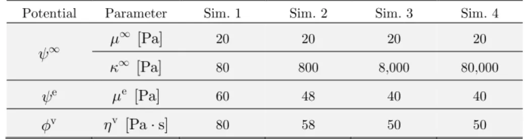
Numerical simulations of these experiments were run with a rigid 1.98 mm diameter spherical indenter and a numerical sample with diameter of 10 mm and height of 4 mm . As can be seen from

Figure 2, the cell sample is considered locally homogeneous and it was discretized by 8,130 quadratic hexahedral elements with reduced integration. Due to symmetry, only a quarter of the sample was modeled. Moreover, frictionless contact was considered in the interface between sample and indent-er.

The finite element simulations presented herein were run in the software Abaqus, where the proposed viscoelastic model was implemented into the user-subroutine UMAT.

(a) (b)

Figure 2: Finite element model employed for the simulations of nanoindentation tests. (a) Perspective view of the model showing the spherical indenter and the cell sample in a quarter symmetry.

(b) Top view of the numerical sample emphasizing the mesh refinement.

Using this finite element setup, a set of numerical simulations evaluated the capability of pre-sent material model to reprepre-sent the experimental data, considering different compressibility levels. To this aim, for increasing values of k¥_{, the parameter m}¥ _{was kept fixed and the viscoelastic} parameters _me _{and h}v _{were adjusted in order to fit the numerical curves to the range of the}

exper-imental data (see Table 1).

Potential Parameter Sim. 1 Sim. 2 Sim. 3 Sim. 4

y¥ m [Pa]

¥ _{20 20 20 20}

[Pa]

k¥ _{80 800 8,000 80,000}

e

y _me _{[Pa] 60 48 40 40}

v

f _hv _{[Pa s]⋅ 80 58 50 50}

Table 1: Constitutive parameters related to the numerical curves shown in Figure 3.

Figure 3-a compares the force-displacement curves of the indenter obtained from the experiments and Simulation 1. Figure 3-b show the corresponding results obtained with all simulations. Finally,

X Y

Z

X Y

Figure 4 depicts the displacement and the von-Mises (Cauchy) stress fields at maximum penetration of the indenter for Simulation 4.

(a) (b)

Figure 3: (a) Comparison between experimental and numerical results obtained from the nanoindentation tests. The experimental points were plotted based on data provided by Nawaz et al. (2012). (b) Sensitivity of the

numerical results in relation to the incompressible response of the model. The related constitutive parameter sets are shown in Table 1.

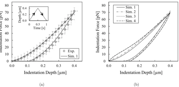
In order to gain a better understanding of how the parameters of Table 1 affect the incompressi-ble response of the model, simulations of homogeneous uniaxial tensile tests were performed. Figure 5-a display the uniaxial first Piola-stretch curves, while the corresponding time history of the Jaco-bians are shown in Figure 5-b. All simulations were run under an engineering strain rate of _{0.05 s}-1_.

(a) (b)

Figure 4: Displacement (a) and von-Mises stress (b) fields at the instant of the maximum penetration of the indenter for Simulation 4.

0 10 20 30 40 50 60 70 80

0.0 0.1 0.2 0.3 0.4

Ind

ent

at

ion

Forc

e

[p

N

]

Indentation Depth [µm]

Exp. Sim. 1

0.0 0.2 0.4

0 0.5 1

D

ept

h

[µ

m

]

Time [s]

0 10 20 30 40 50 60 70 80

0.0 0.1 0.2 0.3 0.4

Inde

nt

at

ion

Forc

e

[pN

]

Indentation Depth [µm]

Sim. 1 Sim. 2 Sim. 3 Sim. 4

Disp. [μm]

0.000 0.040 0.080 0.120 0.160 0.200 0.240 0.280 0.320 0.360

0.400 (von-Mises [Pa])

Cauchy Stress

(a) (b)

Figure 5: Stress-stretch curves (a) and time history of the volumetric jacobians (b) obtained from simulations of homogeneous uniaxial tensile tests. The related constitutive parameter sets are shown in Table 1.

4.2 Cyclic, Stress Relaxation and Creep Tests

Identification procedures often recover material parameters that successfully reproduce the used set of experimental data. However, it is not unusual these parameters fail to predict the behavior of the same material under a mechanical condition different from (but close to) that identified. In order to gain confidence on the behavior of the proposed model using the identified parameters, a brief sensi-tivity analysis considering different mechanical tests was carried out.

The same finite element model of the previous section with constitutive parameters of Simula-tion 1 (Table 1) was used.

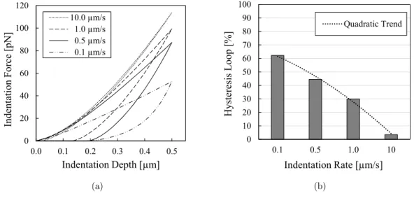
A first set of numerical tests considering cyclic indentations with 0.5 mm depth at indentation rates of 0.1, 0.5, 1.0 and 10 m/sm , was run. The corresponding force-displacement curves are dis-played in Figure 6-a. Different hystereses are seen, depending on the indentation rate. The relative percentage of the energy dissipated at each hysteresis loop is shown in Figure 6-b. Moreover, a quad-ratic trend curve is fitted in order to better illustrate how the dissipated energy changes within the range of indentation rates.

Besides cyclic tests, stress relaxation and creep AFM indentation tests are also found in the lit-erature as efficient experiments to get information on the viscoelastic properties of cells (Haase and Pelling, 2015; Moreno-Flores et al., 2010). Based on this motivation, a set of relaxation and creep simulations under different load conditions were tested, as shown in Figure 7. Concerning the relaxa-tion tests, three indentarelaxa-tion depths of 0.1, 0.3 and 0.5 mm were applied at a 10 m/sm rate, and then the indenter was kept fixed for 10 seconds. The corresponding relaxation curves are displayed in Figure 7-a. Concerning the creep tests, three indentation forces of 10, 25 and 50 pN were progres-sive and linearly applied in 0.05 seconds, and then kept constant for 16 seconds. The corresponding creep curves are shown in Figure 7-b.

0 5 10 15 20 25 30

1.0 1.1 1.2 1.3 1.4 1.5

Sim. 1 Sim. 2 Sim. 3 Sim. 4

0.99 1.00 1.01 1.02 1.03 1.04 1.05 1.06 1.07

0.0 2.0 4.0 6.0 8.0 10.0

Vo

lu

m

et

ric

Ja

cobi

an

Time [s]

(a) (b)

Figure 6: (a) Cyclic nanoindentation tests at different rates. (b) Relative loss of energy by the hysteresis loops computed from cyclic curves.

(a) (b)

Figure 7: Mechanical responses predicted by the viscoelastic model when submitted to nanoindentation tests of stress relaxation (a) and creep (b) under different loading conditions.

5 DISCUSSIONS AND FINAL REMARKS

As can be seen from Figure 3, all numerical simulations were able to predict the local viscoelastic response of fibroblast cells under nanoindentation (in view of the standard deviations) using spheri-cal indenter. In addition, the displacement and stress fields depicted in Figure 4 emphasize the nu-merical results seem to present minimum influence of the boundaries of the sample.

0 20 40 60 80 100 120

0.0 0.1 0.2 0.3 0.4 0.5

Inde

nt

at

io

n

Fo

rc

e

[p

N

]

Indentation Depth [µm]

10.0 µm/s 1.0 µm/s 0.5 µm/s 0.1 µm/s

0 10 20 30 40 50 60 70 80 90 100

0.1 0.5 1.0 10

H

ys

te

re

sis

L

oop

[%

]

Indentation Rate [µm/s]

Quadratic Trend

0 25 50 75 100 125 150

-1 0 1 2 3 4 5 6 7 8 9 10

Ind

ent

at

io

n

Forc

e

[pN

]

Time [s]

0.5 µm 0.3 µm 0.1 µm

0.0 0.1 0.2 0.3 0.4 0.5 0.6 0.7 0.8 0.9

-2 0 2 4 6 8 10 12 14 16

Inde

nt

at

io

n

D

ept

h

[µ

m

]

Concerning to the numerical curves plotted in Figure 3-b, it can be seen that when incompressi-bility is enforced, the force-indentation response changes its curvature within the firsts 0.1 mm dis-placement, diverging from the usual expected behavior. Based on these numerical results, one can hypothesize that cells seem to respond locally, under indentation tests, as a compressible material (see time histories of the volumetric jacobians plotted in Figure 5-b). However, further numerical and experimental investigations are required to support this hypothesis.

Taking into account the cyclic numerical experiments displayed in Figure 6-a one can observe that, for the identified material parameters, the dissipation decreases when the indentation rate increases. The energetic loss is quantified by the hysteresis loop as shown in Figure 6-b. Moreover, one can see the percentage of hysteresis presents a nearly quadratic decay over rates.

According to the relaxation and creep simulations shown in Figure 7, the material reaches equi-librium states beyond 5 seconds in stress relaxation and 10 seconds in creep. These time scales pre-dicted by the model show sound agreement with experimental data reported in Moreno-Flores et al. (2010).

It is worth mentioning the use of analytical expressions based on Hertz contact model and in-dentation tests to estimate the cell stiffness is common in the literature (technical details may be found elsewhere, Vinckier and Semenza (1998)). This approach, however, is quite sensitive to the indentation depth, since the Hertz expressions were tailored for linear elastic materials and infinites-imal strains. In addition, it is unable to consider rate dependent effects. In contrast to these analyti-cal approaches, the finite element simulation procedure presented in this work seems to provide a more accurate tool for a better understanding of stiffness and energetic dissipation of cells.

Within a multiscale numerical framework of biological tissues, the present constitutive model may be employed to represent the microscopic material phases composed of cells and/or other iso-tropic viscoelastic components as well, a necessary step for future developments in the mechanobiol-ogy field, where the knowledge of the complex mechanical responses of cells are issues of major con-cern.

Acknowledgments

The authors would like to thank the financial support provided by the Brazilian funding agencies CAPES - (Coordination for the Improvement of Higher Education Personnel) and CNPq - (Nation-al Council for Scientific and Technologic(Nation-al Development).

Conflict of Interest Statement

The authors have no conflicts of interest.

References

Anand, L., Gurtin, M.E., (2003). A theory of amorphous solids undergoing large deformations with applications to polymers and metallic glasses. International Journal of Solids and Structures 40, 1–29.

Bonakdar, N., Gerum, R., Kuhn, M., Spörrer, M., Lippert, A., Schneider, W., Aifantis, K.E., Fabry, B., (2016). Mechanical plasticity of cells. Nature Materials 1–6.

Bonet, J., Wood, R.D., (2008). Nonlinear continuum mechanics for finite element analysis, 2nd Editio. ed, Zhurnal Eksperimental’noi i Teoreticheskoi Fiziki. Cambridge University Press.

de Souza Neto, E.A., Peric, D., Owen, D.R.J., (2009). Computational Methods for Plasticity: Theory and Applications, Engineering.

Fancello, E., Ponthot, J.-P., Stainier, L., (2006). A variational formulation of constitutive models and updates in non-linear finite viscoelasticity. International Journal for Numerical Methods in Engineering 65, 1831–1864.

Fancello, E., Vassoler, J.M., Stainier, L., (2008). A variational constitutive update algorithm for a set of isotropic hyperelastic-viscoplastic material models. Computer Methods in Applied Mechanics and Engineering 197, 4132–4148. Gurtin, M., Fried, E., Anand, L., (2010). The mechanics and thermodynamics of continua. Cambridge University Press.

Gurtin, M.E., Anand, L., (2005). The decomposition F = FeFp, material symmetry, and plastic irrotationality for solids that are isotropic-viscoplastic or amorphous. International Journal of Plasticity 21, 1686–1719.

Haase, K., Pelling, A.E., (2015). Investigating cell mechanics with atomic force microscopy. Journal of The Royal Society Interface 12.

Hamann, S., Kiilgaard, J.F., Litman, T., Alvarez-Leefmans, F.J., Winther, B.R., Zeuthen, T., (2002). Measurement of Cell Volume Changes by Fluorescence Self-Quenching. Journal of Fluorescence 12, 139–145.

Itskov, M., (2002). The derivative with respect to a tensor: some theoretical aspects and applications. ZAMM - Journal of Applied Mathematics and Mechanics 82, 535–544.

Janmey, P.A., McCulloch, C.A., (2007). Cell mechanics: integrating cell responses to mechanical stimuli. Annual review of biomedical engineering 9, 1–34.

Jirásek, M., Bazant, Z., (2002). Inelastic analysis of structures. John Wiley & Sons, Ltd.

Jog, C.S., (2007). Foundations and Applications of Mechnics Volume I: Continuum Mechanics, 2 edition. ed. Alpha Science Intl Ltd.

Kollmannsberger, P., Fabry, B., (2011). Linear and Nonlinear Rheology of Living Cells. Annual Review of Materials Research 41, 75–97.

Lavagnino, M., Wall, M.E., Little, D., Banes, A.J., Guilak, F., Arnoczky, S.P., (2015). Tendon mechanobiology: Current knowledge and future research opportunities. Journal of Orthopaedic Research 33, 813–822.

Moreno-Flores, S., Benitez, R., Vivanco, M. dM, Toca-Herrera, J.L., (2010). Stress relaxation and creep on living cells with the atomic force microscope: a means to calculate elastic moduli and viscosities of cell components. Nanotechnology 21.

Nawaz, S., Sánchez, P., Bodensiek, K., Li, S., Simons, M., Schaap, I.A.T., (2012). Cell Visco-Elasticity Measured with AFM and Optical Trapping at Sub-Micrometer Deformations. PLoS ONE 7.

Ortiz, M., Stainier, L., (1999). The variational formulation of viscoplastic constitutive updates. Computer Methods in Applied Mechanics and Engineering 7825, 419–444.

Qi, J., Fox, A.M., Alexopoulos, L.G., Chi, L., Bynum, D., Guilak, F., Banes, A.J., (2006). IL-1beta decreases the elastic modulus of human tenocytes. Journal of applied physiology 101, 189–195.

Radovitzky, R., Ortiz, M., (1999). Error estimation and adaptive meshing in strongly nonlinear dynamic problems. Computer Methods in Applied Mechanics and Engineering 172, 203–240.

Simo, J.C., Taylor, R.L., (1985). Consistent tangent operators for rate-independent elastoplasticity. Computer Methods in Applied Mechanics and Engineering 48, 101–118.

Vinckier, A., Semenza, G., (1998). Measuring elasticity of biological materials by atomic force microscopy. FEBS Letters 430, 12–16.

Wang, J.H.C., (2006). Mechanobiology of tendon. Journal of Biomechanics 39, 1563–1582.

Weber, G., Anand, L., (1990). Finite deformation constitutive equations and a time integration procedure for isotropic, hyperelastic-viscoplastic solids. Computer Methods in Applied Mechanics and Engineering 79, 173–202. Zlotek-Zlotkiewicz, E., Monnier, S., Cappello, G., Le Berre, M., Piel, M., (2015). Optical volume and mass measurements show that mammalian cells swell during mitosis. The Journal of Cell Biology 211, 765–774.

APPENDIX A – SOLUTION OF THE LOCAL CONSTITUTIVE PROBLEM

Herein are present the operational details related to the solution strategy employed to solve the variational constitutive principle (3.8). Furthermore, the nonlinear equations resulting from the stationarity condition are solved by the full Newton-Raphson procedure.

A.1 Stationarity Condition

In view of the variational principle (3.8), the stationarity condition is defined through the variation d฀=0, which results in the following equations:

1 1

1

1

1 1

v inc

v v v

cte v cte

d 0

1 0

n n n

n n

n

J

J

g

g

+ + +

+ + ₊

=

=

ìï¶ ¶ ¶

ï _{+ =}

ïï_{¶ ¶ ¶}

ïï

=  í_{ï ¶}

ï _{- =}

ïï¶

=

ïï =

î F

F

0

d d d

 



 . (A.1)

The partial derivatives of (A.1) result in,

(

)

1

e v e _T

v v e

inc

v v t v, v tsym n n n

y f y

-+ +

é ù

¶ ₌¶ _{+ D} ¶ ¶ _{= -D ê ú}

ê ú

¶d ¶d ¶d ¶d ë F F M û



, (A.2)

and,

1 1

1 1

v

v v v v

n

n n n

J

t J

-+

+ +

¶ _{= D}

¶d F F , (A.3)

where Mne+1 :=Cne+1Sne+1 are the elastic Mandel stress tensor.

A.2 Newton-Raphson Procedure

Concerning to the full Newton-Raphson procedure, one can define from the nonlinear equations (A.1) the quantities,

1

1

1 1

v v

: , :

n

n

n n _g

g+ +

+ +

ì ü

ï ï

ï ï

ï ï ìï üï

ï ï _{ï ï}

ï ï

=í =

¶ ¶

¶ ¶

ý í ý

ï ï ï ï

ï ï ï_î ï_þ

ï ï

ï ï

ï ï

î þ

r d x d

 

where r_n+1 is a residual and

1

n+

x represents the set of unknown variables. Therefore, an increment

d related to a current iteration of the Newton’s algorithm, is computed from the linear system of equation,

1

1

1

1 1 1

1

2 2

v

v v v v

2 2 v v : : n n n

n n n

n

d dg

g

d dg

g g g

g + + + + + + + ¶ ₊ ¶ _{= -}¶ ¶ ¶ ¶ ¶ ¶ ¶ ₊ ¶ _{= -} ¶ ¶ ¶ ìïï ïï ïï íï ïï ï

î¶ ¶ ¶

ïï

d

d d d d

d d          

   , (A.5)

which can be represented by the compact arrangement Jn+₁ dxn+₁ = -rn+₁. The symbol  repre-sents the appropriate product between the Newton’s increments dx_n+₁ and the Jacobian matrix

1 1 1 1 1 1 1 2 2

v v v

2 2 v : n n n n n n n g g g g + + + + + + + ¶ ¶ ¶ ¶ ¶ ¶ ¶ = ¶ ¶ ¶ ¶ ¶ ¶ ¶ ì ü ï ï ï ï ï ï ï ï ï ï ï ï

= í_ï ý_ï

ï ï ï ï ï ï ï ï ï ï î þ

d d d

r J x d      

  . (A.6)

In order to achieve the quadratic convergence rate provided by the Newton’s method, the de-rivatives of equation (A.6) must be computed precisely. Accordingly, the second partial dede-rivatives of (A.6) result in

1 1 1 1 1 1 1 1 1 1 1 1 1 1 2

2 2 v 2

v v v inc

v v v v v v v

2 2

v v v

v 0

n

n n n

n

n

n n n

n n n n n J t J t J g g g g g -+ + + + + -+ + + + + + + ì ü ï ï

ï ₌ ï

ï ï ï ï ï ï ï ï í ý ï ï ï ï ï ï ï ï ï ï ï ¶

¶ ₊ ¶ ¶ _{= D}

¶ ₌ ¶ ¶ ¶ ¶ ¶ ¶ ¶ ¶

¶ ¶ _{= D} ¶ ₌

¶ ¶

¶ _ï

î ¶ þ

F F

d d d d d d d

x

F F

d

r       





 

  , (A.7)

where it is introduced the fourth order operators,

1

2 2 e 2 v 2 e

inc

sym sym

v v v v t v v, v v : n : ,

y f y

+

¶ ₌ ¶ _{+ D} ¶ ¶ ₌

-¶ -¶d d ¶ ¶d d ¶ ¶d d ¶ ¶d d   



(

)

(

)

(

)

1 1 1

1

1 1

e T

T

2 v v v v e v v

v

: n n n n n : ,

n

n t n t n

+

- -

-+ + + +

+

é ù

é ù _ê¶ _ú

ê ú

= D + D _{ê ú}

ê ú _¶

ë û ë û

M

F F F F M F F I

d

  

(

)

(

)

1 1 1

1 1

e e e

e e

v : v : v ,

n n n

n n

+ + +

+ +

é ù é ù

¶ _{= ê}¶ _{ú+ ê}¶ _ú

ê ú ê ú

¶ _ë ¶ _{û ë} ¶ _û

M C S

I S C I

d  d  d

1 1

1 1

1

e e

e

sym sym sym

v 2 : : , v : : ,

n

n n

n n

t ₊ t _{+ +}

+ +

¶ ¶

= - D = -D

¶ ¶

C S

d    d   

(

)

1 1 1 1 1 1 2 e

e v v e

e e

: n , : 4 ,

n n n n n n y + + + -+ + + ¶ = = ¶ ¶

C F F I

C C    1 1 1 2 v 2 v sym sym

v v : : ,

n n n J t J + + +

¶ _{= D}

¶ ¶d d   

(

) (

) (

) (

)

1 1 1 1

1

v v v v v v v v

: n n n n n n n n .

n

- - -

-+ + + +

+ = F F Ä F F + F F F F

 

In equations (A.8), _sym is the fourth order symmetric identity tensor. In addition, are intro-duced the tensor products

(

)

( ) ( )

ijkl ij kl

Ä =

A B A B and

(

)

( ) ( )

ijkl = ik jl

AB A B , for any second orders tensors A and B.

APPENDIX B – CONSISTENT MATERIAL TANGENT MODULUS

Taking into account a total Lagrangian formulation (Belytschko et al., 2000), the linearization of the equilibrium equations results in the material tangent modulus

1 1

1 1 1

2 red inc

d d

: 2 4

d d d

n n

n n n

+ +

+ + +

= S =

C C C

  , _(B.1)

where one can note that if red inc

 is a convex potential of Cn+1, the tensor n+1 will present major

symmetry. The total derivative of the second Piola-Kirchhoff stress tensor is given by

1 1 1

1 1 1

v v

d d

:

d d

n n n

n n n

+ + +

+ + +

æ ö

æ ö

¶ _ç¶ _{÷ ç ÷÷}

÷

= _¶ +ç_{çç ÷ ç÷} ç_ç ÷_÷÷

è ¶ ø è ø

S S S d

C C d C



 . _(B.2)

The partial derivatives of (B.2) result in

(

)

1 1

1 1 1

1

sym sym v sym sym

1

: : , : :

2

n n

n n n

n + + + + + + ¥ ¶ ¶ = = ¶ ¶ S S

C     d    , (B.3)

where,

(

)

(

)

1 1 1 1

1 1 1

1 1

2

v v e v v

: 4 , : n n : : n n

n n n

n n

y - - -

-+ + + +

+ + +

+ +

¥

¥ ₌ ¶ ₌

¶C ¶C F F F F

     ,

(

) (

)

1 1 1 1

1 1

1 1

1 1

e

v v e v v

v

: 2 : n

n

n n n n

n t

- - -

-+ + + + +

+

é_¶ ù

é ù ê ú

= - D _{ê ú}+ _{ê ú}

ë û _{ë¶ û}

S

F F S F F

d

   ,

(B.4)

in which the fourth order operators 1

e v

n+

¶S ¶d and

1

e

n+

 were introduced in equations (A.8). The total derivative _d v _{d 1}

n+

d C of equation (B.2) is one of the solutions of the following linear system of equation:

1

1 1 1 1

1

1 1 1 1 1 1

1

2 v 2 2

v v v v

2 v 2 2

v d d : d d d d : d d n

n n n n

n

n n n n n n

n

g g

g

g g g

g + + + + + + + + + + + + +

¶ ₊ ¶ _{Ä = -} ¶

¶ ¶ ¶ ¶ ¶ ¶ ¶ ₊ ¶ _{= -} ¶ ¶ ¶ ¶ ¶ ìïï ïï ïï íï ïï ¶ ï î ¶ ïï d C C

d d d C d

d

C C C

d          

   , (B.5)

1 1

1

1 1 1

1 1 1 1 1

1 1 1 1 1 1 1 1 2 v v 2 , d d : , : d d , d d d d

n n n n n n

n

n n

n n

n

n n n n

n n n

g g + + + + + + + + + + + + + + + + + + + ì ü

ì ü ï ï

ï ï _{ï ï}

ï ï _{ï ï}

ï ï _{ï ï}

ï ï _{ï ï}

ï ï

ï ï ï ï

= í_ï ý_ï =í_ï ý_ï

ï ï ï ï

ï ï ï ï

ï ï ï ï

ï ï ï ï

ï ï

¶

¶ ¶ ¶ ¶ _{¶ ¶}

= - =

î þ ï

¶ ¶ ¶ ¶ ¶

¶ ¶ _ï

î þ

d

x x C C d

x C C x C C

C C

r r r r

J









 . (B.6)

One can note that from equation (B.6), the derivative ¶rn+₁ ¶xn+₁ is the Jacobian matrix previ-ously defined in equation (A.6). Finally, the partial derivatives of the set ¶rn+₁ ¶Cn+₁are computed as 1 1 1 1 1 1 1

2 2 e

sym sym v v 2 : : : _n n n n n n n t y g + + + + + + +

¶ ₌ ¶ _{= -D}

¶ ¶ ¶ ¶ ¶ ¶ ¶ = ì ü ï ï ï ï ï ï ï ï ï ï ï ï

= í_ï ý_ï

ï ï

ï

¶ ¶ ï

ï ï

ï ï

ï ï

î þ

C d C d

r C 0 C      

 , (B.7)

where,

(

)

1 1 1 e T v v

: n n :

n n n+ -+ + + é ù

é ù _ê¶ _ú

ê ú

= _{ê ú ê ú}

¶

ë _{û ë û}

M

F F I

C   ,

(

)

(

)

e e e

e _: e _:

n n n

n n n n n + + + + + +

+ é ù é + ù

¶ _ê¶ _{ú ê}¶ _ú

= _{ê ú}+ _{ê ú}

¶ _ë¶ _{û ë}¶ _û

M C S

I S C I

C  C  C ,

(

)

1 1

1

1 1 1

1 1 1

e e e

e v v

sym

1

: , :

2 n n n

n n n

n n n -

-+ + + + + + + + + é ù

¶ _ê¶ _ú ¶

= _{ê ú} =

¶ _ë¶ _û ¶

S C C

F F

C  C C   .