Daytime SABER/TIMED observations of water vapor in the mesosphere: retrieval approach and first results

www.atmos-chem-phys.net/9/8139/2009/ © Author(s) 2009. This work is distributed under the Creative Commons Attribution 3.0 License.

Chemistry

and Physics

Daytime SABER/TIMED observations of water vapor in the

mesosphere: retrieval approach and first results

A. G. Feofilov1,2, A. A. Kutepov1,2, W. D. Pesnell2, R. A. Goldberg2, B. T. Marshall3, L. L. Gordley3,

M. Garc´ıa-Comas4, M. L´opez-Puertas4, R. O. Manuilova5, V. A. Yankovsky5, S. V. Petelina6, and J. M. Russell III7

1_{The Catholic University of America, 620 Michigan Ave., Washington D.C. 20064, USA} 2_{NASA Goddard Space Flight Center, Mailcode 674, Greenbelt Rd., Greenbelt, MD 20771, USA} 3_{GATS Inc., 1164 Canon Blvd., Suite 101, Newport News, VA 23606, USA}

4_{Instituto de Astrof´ısica de Andaluc´ıa (CSIC), C/Camino Bajo de Huetor, 50, Granada, 18008, Spain} 5_{Institute for Physics, St.Petersburg State University, Ulianovskaja, 1, St. Petersburg, 198904, Russia} 6_{La Trobe University, Victoria, 3086, Australia}

7_{Hampton University, Hampton, VA 23668, USA}

Received: 6 May 2009 – Published in Atmos. Chem. Phys. Discuss.: 26 June 2009 Revised: 5 October 2009 – Accepted: 12 October 2009 – Published: 2 November 2009

Abstract.This paper describes a methodology for water va-por retrieval in the mesosphere-lower thermosphere (MLT) using 6.6µm daytime broadband emissions measured by SABER, the limb scanning infrared radiometer on board the TIMED satellite. Particular attention is given to account-ing for the non-local thermodynamic equilibrium (non-LTE) nature of the H2O 6.6µm emission in the MLT. The non-LTE H2O(ν2) vibrational level populations responsible for this emission depend on energy exchange processes within the H2O vibrational system as well as on interactions with vi-brationally excited states of the O2, N2, and CO2molecules. The rate coefficients of these processes are known with large uncertainties that undermines the reliability of the H2O re-trieval procedure. We developed a methodology of finding the optimal set of rate coefficients using the nearly coinciden-tal solar occultation H2O density measurements by the ACE-FTS satellite and relying on the better signal-to-noise ratio of SABER daytime 6.6µm measurements. From this compari-son we derived an update to the rate coefficients of the three most important processes that affect the H2O(ν2) populations in the MLT: a) the vibrational-vibrational (V–V) exchange between the H2O and O2 molecules; b) the vibrational-translational (V–T) process of the O2(1) level quenching by collisions with atomic oxygen, and c) the V–T process of the H2O(010) level quenching by collisions with N2, O2, and O. Using the advantages of the daytime retrievals in the MLT, which are more stable and less susceptible to uncertainties

Correspondence to:A. G. Feofilov ([email protected])

of the radiance coming from below, we demonstrate that applying the updated H2O non-LTE model to the SABER daytime radiances makes the retrieved H2O vertical profiles in 50–85 km region consistent with climatological data and model predictions. The H2O retrieval uncertainties in this approach are about 10% at and below 70 km, 20% at 80 km, and 30% at 85 km altitude.

1 Introduction

therein). These particles are responsible for such phenomena as noctilucent clouds (NLCs) and polar mesospheric sum-mer echoes (PMSEs, see also Appendix A for the abbrevia-tions not explained in the text for readability’s sake). Due to high sensitivity to local kinetic temperatures, the NLC and PMSE phenomena can be used as temperature probes for these regions (e.g. L¨ubken et al., 2007; Petelina and Zaset-sky, 2009) and as possible indicators of climate change (e.g. Thomas, 2003). NLCs have also been used as tracers of Shut-tle rocket engine exhausts when an extraordinary amount of water was injected into the atmosphere causing an increase in NLC brightness (Siskind et al., 2003; Stevens et al., 2003, 2005).

Water vapor measurements in the MLT region have been performed since the 1970s utilizing ground- and aircraft-based microwave measurements (Croom et al., 1977; Bevilacqua et al., 1983; Hartogh et al., 1995; see also refer-ences in Brasseur and Solomon, 2005, Sect. 4.1.1). Space-borne measurements of the water vapor altitude distributions started in 1978 with the launch of the Nimbus-7 spacecraft observatory that utilized the SAMS (Drummond et al., 1980) and the LIMS (Gille et al., 1980) instruments for water va-por observations. Since then water vava-por has been measured by a number of space experiments: HALOE (Russell et al., 1993), ISAMS (Taylor et al., 1993), ATMOS (Gunson et al., 1996), CRISTA-1,2 (Offermann et al., 1999; Grossmann et al., 2002), and others. Six satellite-borne instruments are cur-rently performing water vapor measurements in the upper at-mosphere: the ACE-FTS/Scisat-1 (Bernath et al., 2005) and SOFIE/AIM (Gordley et al., 2009) instruments use an oc-cultation technique, while MLS/Aura (Waters et al., 1999), SMR/Odin (Murtagh et al., 2002), SABER/TIMED (Russell et al., 1999), and MIPAS/Envisat (Fischer et al., 2008) mea-sure atmospheric emission in the limb.

Most of the methods used for inversion of infrared radia-tion data obtained in the limb viewing geometry are based on the solution of the radiative transfer problem under the as-sumption of local thermodynamic equilibrium (LTE) (Gille and Russell, 1984; Barnet, 1987). However, above about 55 km altitude the vibrational H2O(ν2)levels, which give rise to the bands providing the main contribution to the 6.6µm SABER channel, are out of LTE (L´opez-Puertas and Tay-lor, 2001). As a result, water vapor density retrievals in the MLT require solving the non-LTE problem for the popula-tions of H2O vibrational levels. Non-LTE also complicates the retrieval process by making the entire problem non-local in altitudes, with the variation of the H2O density at one al-titude affecting the H2O levels populations at other alal-titudes, especially in the MLT region. For these kinds of tasks, the forward fitting iterative approach is preferable (Gusev, 2003) enabling one to adjust the non-LTE populations at different altitudes to an iteratively changing profile of the retrieved at-mospheric constituent.

In this paper we describe the SABER instrument, its 6.6µm limb emission observation of the MLT (Sect. 2), and

the current status of the H2O non-LTE models (Sect. 3). Sec-tion 4 presents the computer code package ALI-ARMS and the retrieval algorithm applied in this study. In Sect. 5 we present a sensitivity study of the non-LTE model to the varia-tion of a number of rate coefficients of energy exchanges pro-cesses influencing the populations of H2O vibrational levels during daytime. We demonstrate how the broadband 6.6µm emission simulations required for the H2O density retrieval are affected by the uncertainties in available rate coefficients. Using the simultaneous common volume measurements per-formed by the SABER instrument and ACE-FTS occultation experiment which is not affected by non-LTE effects, we il-lustrate that a revision of certain rate coefficients is required for an adequate interpretation of broadband 6.6µm non-LTE H2O emissions. In this section we describe the approach for the rate coefficients fitting and suggest an update to values of these rate coefficients. In Sect. 6 we present the results of preliminary SABER H2O mixing ratio retrievals obtained by applying the updated H2O non-LTE model and show that these retrievals are in a good agreement with other observa-tions and models. Section 7 bridges results obtained with the ALI-ARMS research code and those obtained with this code to the operational retrieval. The latter will be used to pro-duce H2O distributions in the next release of SABER data. This section also describes the SABER Operational Process-ing Code (SOPC) that is based on the GRANADA research code and discusses the retrieval uncertainties linked with the optimization of the research code for operational uses. The main results of the paper are summarized in the Sect. 8.

2 SABER instrument on the TIMED satellite

3 H2O 6.6µm radiance measured by SABER

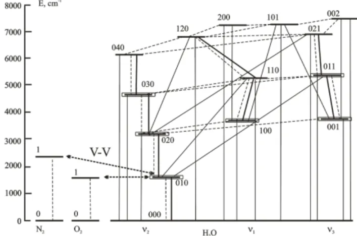
In the gas phase, water molecule vibrations involve combina-tions of symmetric stretch (ν1), covalent bond bending (ν2), and asymmetric stretch (ν3)modes with the band strength ra-tio for the fundamental bands of the main H2O isotope being 0.07/1.50/1.00 for theν1,ν2, andν3vibrations, respectively (Goody and Young, 1995, and references therein; Rothman et al., 2005). The diagram in Fig. 1 shows the ground and various excited vibrational levels of H2O molecule up to 7445 cm−1. The levels are marked in accordance with the number of vibrational quantaν1ν2ν3. The 6.6µm radiance measured in the water vapor channel of the SABER instru-ment arises from the optical transitions from vibrationally excited states with1ν2=1, where 1ν2 denotes the change in theν2vibrational quanta number.

3.1 LTE and non-LTE conditions in H2O

The interpretation of SABER 6.6µm limb radiance profiles requires the information on populations of the correspond-ing H2O vibrational levels at the altitudes of limb obser-vations. In the lower atmosphere the frequency of inelas-tic molecular collisions is sufficiently high, so that these collisions overwhelm other population/depopulation mech-anisms of the molecular vibrational levels. This leads to a local thermodynamic equilibrium, and the populations fol-low the Boltzmann distribution governed by the local kinetic temperature Tkin. In the MLT, where the frequency of in-elastic collisions is much lower than that at lower altitudes, other processes also influence the population of H2O vibra-tional levels. These include: a) the direct absorption of so-lar radiance by the H2O vibrational-rotational bands in the 1.4–6.3µm spectral region; b) absorption of the 6.6µm radi-ance coming from the warmer and denser lower atmosphere; c) vibrational-translational (V–T) energy exchanges by col-lisions with molecules and atoms of other atmospheric con-stituents; d) collisional vibrational-vibrational (V–V) energy exchange with other molecules. As a result, LTE no longer applies in this altitude region and the populations must be found by solving the self-consistent system of kinetic and radiative transfer equations, which express the balance rela-tions between various excitation/excitation processes de-scribed above.

3.2 Non-LTE model of H2O

In this work we use two non-LTE models of water vapor developed by different groups. The first one, with 7 vi-brational levels and 10 ro-vivi-brational bands was developed by L´opez-Puertas et al. (1995) and updated in the book by L´opez-Puertas and Taylor (2001). The second one, with 14 vibrational levels and 33 ro-vibrational bands was developed by Manuilova et al. (2001). The levels included in the models are shown in Fig. 1 where the thick horizontal lines represent

Fig. 1. Vibrational levels, 6.6µm optical transitions (thick solid lines), other optical transitions (thin solid lines), and V–V, V–T en-ergy exchange processes (dashed lines) for H2O non-LTE model. Thick boxed lines correspond to an optimized set of levels used in SOPC.

the vibrational levels of H2O, O2, and N2molecules while the boxed thick lines refer to the H2O levels in the model of L´opez-Puertas et al. (1995). The lowest vibrational levels of the O2and N2molecules coupled by V–V exchange with those of H2O are also shown in Fig. 1. The dashed lines on Fig. 1 correspond to the V–V and V–T transitions listed in Table 1 (L´opez-Puertas and Taylor, 2001; Manuilova et al., 2001). Thin solid lines show the optical transitions between H2O levels. Spectroscopic information for these transitions is taken from the HITRAN 2004 database (Rothman et al., 2005).

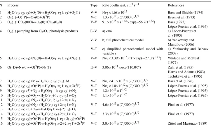
Table 1.Collisional processes involved in the nominal H2O non-LTE model.

N Process Type Rate coefficient, cm3s−1 References

1 H₂O(ν₁;ν₂;ν₃)+O₂(0)↔H₂O(ν₁;ν₂1;ν₃)+O₂(1) V–V Nν₂×1.68×1012 Bass and Shields (1974) 2 O₂(1)+O(3P)↔O₂(0)+O(3P) V–T 1.3×1012×(T /300.0)1/2 Breen et al. (1973) 3 O₂(1)+CO₂(000)↔O₂(0)+CO₂(0₂0) V–V 9.1×1015×T1/2×exp(−56.7/T1/2) Bass (1973)

L´opez-Puertas et al. (1995) 4 O₂(1) pumping from O₂/O₃photolysis products E–V, a)ǫ=4 a) L´opez-Puertas et

al. (1995) V–V, b) full photochemical model b) Yankovsky and

Manuilova (2006) V–T c) simplified photochemical model with

variableǫ

c) Yankovsky and Babaev (2009)

5 H₂O(ν₁;ν₂;ν₃)+N₂(0)↔H₂O(ν₁;ν₂1;ν₃)+N₂(1) V–V Nν₂×3.39×1015×T×exp(−27.0/T1/3) Whitson and McNeal (1977)

6 O(1D)+N₂(0)↔O(3P)+N₂(1) E–V 3.06×1011×exp(110.0/T) Zahr et al. (1975) Harris and Adams (1983) Tachikawa et al. (1995) 7 H₂O(ν₁;ν₂;ν₃)+M↔H₂O(ν₁;ν₂1;ν₃)+M V–T Nν₂×4.1×1014×(T /300.0)1/2 Bass et al. (1976) 8 H₂O(ν₁;ν₂;ν₃)+O(3P)↔H₂O(ν₁;ν₂1;ν₃)+O(3P) V–T Nν₂×1.0×1012×(T /300.0)1/2 L´opez-Puertas et al. (1995) 9 H₂O(ν₁;ν₂;ν3)+N₂↔H₂O(ν₁+1;ν₂;ν₃1)+N₂ V–T 1.2×1011×T1/2 L´opez-Puertas et al. (1995) 10 H₂O(ν₁;ν₂;ν₃)+O₂↔H₂O(ν₁+1;ν₂;ν₃1)+O₂ V–T 1.1×1011×T1/2 L´opez-Puertas et al. (1995) 11 H₂O(ν₁;ν₂;ν₃)+N₂↔H₂O(ν₁1;ν₂+2;ν₃)+N₂

12 H₂O(ν₁;ν₂;ν₃)+N₂↔H₂O(ν₁;ν₂+2;ν₃1)+N₂ V–T 4.6×1013×(T /300.0)1/2 Finzi et al. (1977) 13 H₂O(ν₁;ν₂;ν3)+O₂↔H₂O(ν₁1;ν₂+2;ν₃)+O₂

14 H₂O(ν₁;ν₂;ν₃)+O₂↔H₂O(ν₁;ν₂+2;ν₃1)+O₂ V–T 3.3×1013×(T /300.0)1/2 Finzi et al. (1977) 15 H₂O(ν₁;ν₂;ν₃)+O(3P)↔H₂O(ν₁1;ν₂+2;ν₃)+O(3P)

16 H₂O(ν₁;ν₂;ν₃)+O(3P)↔H₂O(ν₁;ν2+2;ν₃1)+O(3P) V–T 3.0×1012×(T /300.0)1/2 Zittel and Masturzo (1989)

In this tableT is temperature in K and Nν₂is the number ofν₂-quanta.

(L´opez-Puertas and Taylor, 2001). Besides exchanging en-ergy with O2(v) levels, the H2O(ν2)levels interact with N2 levels pumped through collisions with the electronically ex-cited oxygen atoms O(1D) (Zahr et al., 1975; Harris and Adams, 1983; Tachikawa et al., 1995; Edwards et al., 1996). The non-LTE effects in populations of H2O vibrational levels for the daytime conditions in a typical atmospheric scenario are shown in Fig. 2a. The non-LTE calculation for the case study in this plot was performed with the help of the research code ALI-ARMS (see Sect. 4 below) for mid-latitude conditions measured by the SABER instrument (June 23, 2002, lat=39.6◦N, lon=256.2◦E, solar zenith an-gleθz=79.58◦). The H2O VMR profile was taken from the output of the LIMA (Leibniz-Institute Middle Atmosphere) model (Sonnemann et al., 2005; Berger, 2008) for the cor-responding mid-latitude conditions. The profiles of other at-mospheric gases required for the calculations (N2, O2, CO2, O, and O1D) were taken from the corresponding SABER at-mospheric model. The kinetic temperature profile and all VMR profiles were smoothed with a 4 km vertical window for demonstration purposes. The populations of the levels in Fig. 2a are represented by vibrational temperaturesTvib that describe the excitation degree of the levell against the ground level 0:nl/n0=gl/g0exp[–(El−E0)/k/Tvib], where El is the energy of the levell,E0is the energy of the ground

Fig. 2. Non-LTE effects in H2O vibrational levels. Simulation for mid-latitude conditions (23 June 2002, lat=39.6◦N, lon=256.2◦E, θz=79.58◦):(a)vibrational temperatures of H2O levels;(b) contri-butions of different radiative transitions to 6.6µm SABER channel. “Rest” is for contribution from optical transitions other than 020-010 and 020-010-000 involved in the model in Fig. 1.

Tvib>Tkin then the net pumping of the level is larger than that under LTE conditions. Similarly, ifTvib<Tkin, the level is populated less efficiently and/or depopulated faster than at LTE.

The curves in Fig. 2a are marked in accordance with the level nomenclature from Fig. 1. One can see that theTvib of different vibrational levels demonstrate different behav-ior. The populations of 010 and 020 levels depart from LTE above∼55 km altitude while levels such as 030, 100, 011, 110, 040, 021, 120, 002, 101, and 200 show the effects of strong solar pumping down to the troposphere. The pop-ulations of the 001 and 100 levels are close to LTE below

∼45 km altitude though LTE is disturbed both by weak ab-sorption of solar radiance in line wings and by pumping from the upper levels. The contributions of various bands to the simulated SABER 6.6µm radiance are shown in Fig. 2b. The figure demonstrates that the fundamentalν2band (010–000 transition) dominates the 6.6µm radiance at all altitudes with∼15–20% contribution of the first hot band transition (020–010) in the altitude range of 60–100 km. Though there is no direct contribution of the transitions from the upper vi-brational levels, these levels must be included in the daytime calculations since they pump the 010 and 020 levels through a series of V–V and V–T exchanges as well as through radia-tive transitions. The indirect contribution of the upper levels to the daytime 6.6µm radiance measured by SABER was calculated and put on Fig. 2b to be compared with the con-tributions of the 010–000 and 020–010 transitions (see the dashed line in Fig. 2b). One can see that approximately 30% of the daytime signal in the SABER water vapor channel near 85 km is due to pumping the 020 and 010 levels from the up-per levels.

4 ALI-ARMS research code

Most of the calculations performed in this work were made using the ALI-ARMS computer code (see Kutepov et al., 1998; Gusev and Kutepov, 2003; and references therein) that solves the multi-level problem using the Accelerated Lambda Iteration (ALI) technique developed for calculating non-LTE populations of atomic and ionic levels in stellar at-mospheres (Rybicki and Hummer, 1991). The code itera-tively solves a set of statistical equilibrium equations and the radiative transfer equations. The algorithm efficiency is en-sured by the ALI technique, which avoids the expensive ra-diative transfer calculations for the photons trapped in the op-tically thick cores of spectral lines. The ALI-ARMS model was successfully applied by Kaufmann et al. (2002, 2003) and Gusev et al. (2006) to the non-LTE diagnostics of spec-tral Earth’s limb observations from the CRISTA instrument (Offermann et al., 1999; Grossmann et al., 2002). Kutepov et al. (2006) used this model to validate the SOPC used for temperature retrievals from the 15µm CO2emissions mea-sured by SABER. The retrieval method implemented in the

ALI-ARMS code is similar to that used in the SOPC, which is based on an iterative onion-peel technique using the relax-ation method described in Gordley and Russell (1981). The process starts with the initial guess on a water vapor profile combined with a fixed atmospheric model (pressure, tem-perature, and VMRs of atmospheric gases retrieved from a corresponding SABER measurement). The non-LTE popu-lations are calculated and used for monochromatic limb ra-diances calculations for each limb-path that are convolved with the instrumental function for SABER water vapor chan-nel. The resulting simulated radianceI is compared to the measured radiance at each tangent height, and the water va-por VMR is iterated using the following relaxation scheme: ξi+1=ξi+(Imeas−Ii) / (∂I/∂ξ), where ξi+1 and ξi are the water vapor VMRs at thei+1-th andi-th iterations, respec-tively,Imeasis the limb radiance measured by SABER,I iis the simulated limb radiance at thei-th iteration, and (∂I/∂ξ) is the numerically calculated derivative of the radiance pro-duced by the forward model with respect toξ. After all limb-paths are converged, a new H2O VMR profile is produced, and new non-LTE populations of H2O molecular levels are calculated, the radiance is simulated again. The iterations are repeated until the differences between the simulated and measured radiances become equal to the radiance noise in the channel.

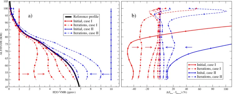
Figure 3 shows the self-consistency check of the retrieval procedure performed for the model atmosphere discussed in Sect. 3.1. First, the non-LTE task was solved for the refer-ence H2O profile, and the limb radiance was calculated using the non-LTE populations of the H2O levels, observation ge-ometry, and the SABER instrumental function. Second, the resulting radiance profile was used as the “measured” profile (Imeas). Two tests were then conducted. The initial guess H2O VMR profile was set equal to 1.0×10−6(case I) and 1.0×10−5(case II) in the 50–100 km altitude range. Below and above this range the original values of the H2O profile were used. The retrieval procedure was run for both cases. Figure 3a shows that the retrieved H2O profile rapidly con-verges to the reference profile in the course of iterations and that the result does not depend on the initial profile. Figure 3b demonstrates the difference between the simulated and refer-ence radiances at each iteration. One can see that the con-verged radiance profile reproduces the reference profile at all points in the 50–100 km altitude range.

Fig. 3.Self-consistent retrievals of H2O density in the 50–100 km altitude range:(a)iterations starting with two different initial guess H2O VMR profiles: 1.0×10−6(case I) and 1.0×10−5(case II);(b)percent difference between the reference and calculated radiance profiles in the course of iterations for cases I and II.

point. This scenario is realized if either the H2O VMR or vibrational levels pumping falls rapidly with altitude. Fortu-nately, the H2O VMR profiles in the Earth’s atmosphere do not experience rapid falloffs when moving from top to bot-tom. To avoid the problem of insufficient levels pumping, we do not consider the nighttime cases or the measurements for whichθz≥88.0◦.

5 Validating the non-LTE H2O model

The accuracy of non-LTE modeling depends on the quality of the experimental and theoretical rate coefficients describ-ing the populatdescrib-ing and de-populatdescrib-ing of the H2O vibrational states that are listed in Sect. 3. The largest source of error in the non-LTE area (above 65–70 km altitude) comes from the uncertainties in V–V and V–T rates (Manuilova et al., 2001). In this section we show the results of a sensitivity study per-formed for the H2O non-LTE model, describe the method that was applied to validating the set of rate coefficients used in the model, and suggest an update to some of these coeffi-cients.

5.1 Sensitivity study

We examined the sensitivity of H2O(ν2), and especially the H2O(010), populations to variations of V–V rates, V–T rates, and effective quantum yield ε for various atmo-spheric scenarios. We also estimated the effects of tem-perature uncertainties both in the LTE dominated and in the non-LTE dominated areas. Here we discuss the results for three test cases: tropical, mid-latitude winter, and po-lar summer (Figs. 4, 5, and 6, respectively). The

atmo-spheric pressure-temperature profiles as well as profiles of other atmospheric gases, except H2O, were taken from the current V1.07 SABER dataset (http://saber.gats-inc.com/). The parameters of the SABER scans used for sensitivity study are: lat=1.23◦S, lon=7.24◦E, θz=26.62◦ for tropics; lat=42.14◦S, lon=11.2◦E,θz=64.12◦ for mid-latitude win-ter; lat=73.56◦_{N, lon=22.59}◦_{E, θ}

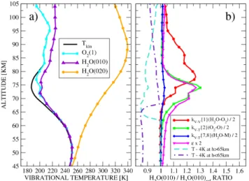
Fig. 4. Sensitivity study for the tropical case. (a) Tempera-ture profile retrieved from SABER and vibrational temperaTempera-tures of H₂O(010), H₂O(020), and O₂(1) levels. (b)Sensitivity of the H2O(010) population tokV−V{1}(H2O–O2),kV−T{2}(O2–O), and

kV−T{7,8}(H2O–M) rate coefficients and to local temperature vari-ations.

must lead to a decrease in H2O(010) population at altitudes above 65–70 km for the tropical and mid-latitude modes. This is also true for polar summer up to∼104 km altitude, where the H2O(010) vibrational temperature crosses the ki-netic temperature profile and the effect reverses. Similarly, an increase of the H2O(010)–O2(1) V–V rate will lead to a more efficient de-population of the H2O(010) level and, as a result, to a H2O(010) population decrease in the 65–95 km altitude range, with the effect depending on the model. Us-ing the same logic one can conclude that an increased O2(1) quenching will result in a decreased H2O(010) population and, finally, that the enhanced O2(1) pumping will cause the H2O(010) level population to increase.

Having this in mind we tested the sensitivity of the H2O(010) population to each of the following processes: H2O(ν2)–O2(1), H2O(ν2)–N2(1), and O2(1)–CO2(020) V–V exchanges, and H2O(ν2)–O2, H2O(ν2)–N2, H2O(ν2)–O, O2(1)–O2, O2(1)–N2, and O2(1)–O V–T quenching, and quantum yieldεfor the O2(1) pumping. First, we performed a reference run for each atmospheric scenario with the rates from Table 1. Then, a series of test runs were made. For all test runs we fixed the rates in the non-LTE model except for one that was decreased to half its nominal value. We be-lieve that for the purposes of our test, the rate decrease is more representative than its increase since the latter drives the level populations closer to LTE or to LTE in a group of levels while the former “decouples” the level from the other ones and/or from LTE. We also performed the runs with doubled quantum yieldε=8 to estimate the sensitivity of the H2O(010) population to O2(1) level pumping. For each test run the resulting H2O(010) populations at differ-ent altitudes were compared to the reference ones. The

re-Fig. 5.Sensitivity study for the mid-latitude winter case.(a) Tem-perature profile retrieved from SABER and vibrational temTem-peratures of H2O(010), H2O(020), and O2(1) levels. (b)Sensitivity of the H₂O(010) population tokV−V{1}(H2O–O2),kV−T{2}(O2–O), and

kV−T{7,8}(H2O–M) rate coefficients and to local temperature vari-ations.

Fig. 6. Sensitivity study for the polar summer case. (a) Temper-ature profile retrieved from SABER and vibrational temperTemper-atures of H2O(010), H2O(020), and O2(1) levels. (b)Sensitivity of the H2O(010) population tokV−V{1}(H2O–O2),kV−T{2}(O2–O), and

k_V−T{7,8}(H₂O–M) rate coefficients and to local temperature vari-ations.

in the set of three model atmospheres. For convenience we will refer to the processes from Table 1 using their type, number in the table, and the molecules/atoms involved in the reactions: kV−V{1}(H2O–O2), kV−T{2}(H2O–M), and so on. The highest sensitivity of the H2O(010) population and, therefore, of the 6.6µm radiance in the 65–100 km al-titude range is to kV−V{1}(H2O–O2) andkV−T{2}(O2–O) rate coefficients though their importance varies for differ-ent atmospheric models: in the polar summer and trop-ical cases the H2O(010) population is more sensitive to kV−V{1}(H2O–O2)while in the mid-latitude case the effects from kV−V{1}(H2O–O2) and kV−T{2}(O2–O) rates, and from doubling the quantum yield, are comparable. The com-bined effect ofkV−T{7}(H2O–N2,O2)andkV−T{8}(H2O–O) rates is less pronounced in all three scenarios reaching 5% only in the polar summer case.

Other parameters and factors that affect the H2O(010) population are (from most to least im-portant): kV−V{3}(O2–CO2), kV−V{5}(H2O–N2), kE−V{6}(O1D–N2), utilizing the simplified photochem-ical pumping of O2(1) from O3 photolysis with constant profile of quantum yield ε, reducing the number of vi-brational levels in the H2O model from 11 to 7, and kV−T{9}(H2O–N2)through kV−T{16}(H2O–O). The small effect of replacing the complicated scheme of O2/O3 pho-tolysis product kinetics with the constant quantum yield profile needs an explanation. As follows from Manuilova et al. (2001) and Yankovsky and Babaev (2009) the simplified model does not provide an accurate estimate of O2(1) pumping. However, utilizing it for the H2O non-LTE task appears to be reasonable. As the corresponding curves in Figs. 4b, 5b, and 6b show, the sensitivity to O2(1) pumping peaks at∼70–80 km altitude and becomes small at altitudes below∼60 km and above∼80 km. Below∼60 km the O2(1) pumping is masked by LTE processes since any extra source is rapidly thermalized by frequent collisions. On the other hand, O2(1) pumping above 80 km does not strongly affect the H2O(010) populations since the V–V exchange decreases with decreasing pressure. Therefore, one can use a fixed quantum yield model for the purposes of H2O VMR retrieval because this model adequately describes the quantum yield in 60–80 km altitude range while avoiding the expensive O2/O3photolysis product kinetics calculations. For the sake of accuracy, we suggest that H2O non-LTE models replace the constant quantum yieldε=4 with the average quantum yield profile estimated by Yankovsky and Babaev (2009). According to this work,ε=8 at 50 km altitude and falls with the altitude increase toε=6 at 71 km, ε=4 at 80 km, ε=1.5 at 90 km. It almost reaches zero at 100 km altitude. This profile was used in the current study.

5.2 Sensitivity to local temperature

Apart from being sensitive to rate coefficients of various processes, the H2O(ν2)populations and, consequently,

ra-diances in the 6.6µm channel depend on local temperatures. Correspondingly, one has to estimate the possible effects of temperature uncertainty and bias prior to non-LTE model val-idation. This is of particular importance since recent esti-mates performed by Remsberg et al. (2008) show that the accuracy of the SABER temperature retrieval is about±2 K in the upper stratosphere and lower mesosphere. At the same time, SABER V1.07 temperatures (Remsberg et al., 2008; J.-H. Yee, private communications, 2009) show up to a 4 K negative bias in comparison with other measurements in the upper stratosphere and lower mesosphere. We performed the temperature sensitivity studies for all three atmospheric sce-narios described above using the following approach. As one can see from Figs. 4a, 5a, and 6a, the approximate “LTE/non-LTE threshold” for all three atmospheric models is at∼65 km altitude. Accordingly, two test runs for each atmosphere were made to estimate the local and non-local effects of tem-perature profile variation on water vapor retrieval. First, the temperature profile was modified in accordance with the for-mula:

Tnew(z)=Told(z)−4.0×{1−exp[−(h(z)−hthreshold)]}, whereTnew(z)is modified temperature value at the altitude pointz,Told(z)is unperturbed temperature,h(z) is altitude at pointzin km, andhthresholdis a threshold altitude in km. For the first test profile the formula was applied for all alti-tudesh(z)>hthreshold= 62.0 km. The second test profile was obtained by applying the correction defined by the formula: Tnew(z)=Told(z)–4.0×{1−exp[−(hthreshold−h(z))]} for all altitudesh(z)<hthreshold= 68.0 km. The results of the tests are shown on Figs. 4b, 5b, and 6b, where the temperature sensitivity curves are in agreement with the non-LTE effects plotted on Figs. 4a, 5a, and 6a. For all cases considered here decreasing the temperature in the LTE area results in decreas-ing the H2O(010) population at all altitude levels where the correction was made. Moreover, the sensitivity of H2O(010) populations in the MLT to temperature changes in the strato-sphere and lower mesostrato-sphere clearly shows that the absorp-tion of radiance coming from below pumps the H2O(010) levels in the MLT. On the other hand, decreasing the temper-ature in non-LTE area has no effect on the H2O(010) popula-tion in the lower atmospheric layers though it still affects the H2O(010) populations locally. This effect decreases as the altitude increases and is less pronounced in the polar summer mesosphere in comparison with the tropical and mid-latitude cases. However, all three model cases demonstrate sensitiv-ity of the H2O(010) population and, consequently, the wa-ter vapor retrieval, to kinetic temperature variations up to

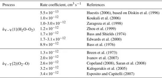
Table 2.Various measurements ofkV−V{1}(H2O–O2)andkV−T{2}(O2–O) rate coefficients.

Process Rate coefficient, cm3s−1 References

kV−V{1}(H2O–O2)

5.5×10−13 Huestis (2006), based on Diskin et al. (1996) 1.0×10−12 Koukuli et al. (2006)

1.0–3.0×10−12 Zaragoza et al. (1998) 1.2×10−12 Zhou et al. (1999) 1.7×10−12 Bass and Shields (1974) 1.7–3.1×10−12 Edwards et al. (2000) 8.9×10−12 Bass et al. (1976)

kV−T{2}(O2–O)

1.3×10−12 Breen et al. (1973) 2.0×10−12 Ivanov et al. (2007)

2.6×10−12 Copeland (2008), Saran et al. (2008) 3.2×10−12 Kalogerakis et al. (2005)

3.4×10−12 Esposito and Capitelli (2007)

5.3 ACE-FTS occultation measurements

The Atmospheric Chemistry Experiment (ACE) on the SCISAT-1 platform, is a Canadian satellite for the remote sensing of the Earth’s atmosphere that has been in opera-tion since August 2003. The primary instrument on ACE is a Fourier-Transform Spectrometer (FTS) with 0.02 cm−1 spectral resolution. Working primarily in the solar occulta-tion observaocculta-tion mode, it provides vertical profiles of temper-ature, pressure, and the VMRs for 18 atmospheric molecules in the 10–100 km altitude range at 4 km vertical resolution over the latitudes 85◦S to 85◦N (Bernath et al., 2005). Trace gas concentrations are retrieved from absorption features in microwindows, i.e. small (∼0.3–1.0 cm−1) portions of the spectrum that contain spectral features related to a molecule of interest with minimal spectral interference from other molecules (Boone et al., 2005; Boone et al., 2007). One ad-vantage of using solar occultation for trace gases retrievals in the MLT is its independence from non-LTE issues since the instrument high spectral resolution allows tracking only the transitions from the ground state whose population can be considered to be equal to the total density of the specie. Recently, the comprehensive validation of the ACE-FTS wa-ter vapor profiles (Lambert et al., 2007; Carleer et al., 2008) has shown that the accuracy of H2O measurements is bet-ter than 5% in the 15–70 km altitude range and is betbet-ter than 10% up to 82 km altitude. This makes the ACE-FTS mea-surements a suitable correlative dataset for comparison with SABER measurements.

5.4 Rate coefficients validation

As follows from Sect. 5.1, the H2O(010) population and, consequently, of retrieved H2O concentration or VMR, are most sensitive to the rates of the following processes: H2O(ν2)–O2(1) V–V exchange, O2(1)–O V–T quenching,

and H2O(ν2)–N2,O2,O V–T quenching with the correspond-ing rate coefficients kV−V{1}(H2O–O2), kV−T{2}(O2–O), andkV−T{7,8}(H2O–M). HereM stands for N2, O2, and O, while {7,8}refers to the 7-th and 8-th rows in Table 1, respectively. The measured and theoretically estimated val-ues of kV−V{1}(H2O–O2) and kV−T{2}(O2–O) rate coef-ficients are given in Table 2. Apparently, the value of kV−V{1}(H2O–O2)rate coefficient varies by more than an order of magnitude, and the largest value ofkV−T{2}(O2–O) is 2.5 times the smallest one. The estimates for the uncertain-ties ofkV−T{7,8}(H2O–M)from the work of Bass (1981) are of the same order as for thekV−T{2}(O2–O). These uncer-tainties require searching for an optimal set of rates that will give the best agreement of the non-LTE measurement with reference climatologies and/or datasets.

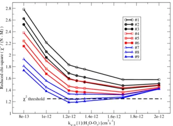
Fig. 7. Validation of the H2O non-LTE model using simultane-ous common volume measurements of SABER and ACE-FTS. Each point represents a reduced χ2 value calculated for a cer-tain combination of kV−V{1}(H2O–O2), kV−T{2}(O2–O) and

kV−T{7,8}(H2O–M) rates over 40 test atmospheres at the al-titudes 60–85 km. Abscissa refers to kV−V{1}(H2O–O2) rate coefficient values, while the shape and shading of the sym-bols define the kV−T{2}(O2–O) and kV−T{7,8}(H2O–M) rate coefficients. Circles: kV−T{2}(O2–O)=1.8×10−12cm3s−1; Squares: kV−T{2}(O2–O)=2.6×10−12cm3s−1; Triangles:

kV−T{2}(O2–O)=3.3×10−12cm3s−1; No symbol filling:

kV−T{7,8}(H2O–M)/1.4; Meshed symbol filling: nomi-nal kV−T{7,8}(H2O–M) from Table 1; Solid symbol filling:

kV−T{7,8}(H2O–M)×1.4.

profiles used for this validation was 40. The SABER data for each coincident ACE-FTS scan were selected using the “overlapping weight” value estimated from the empirical for-mula:γ=1t×4+1η×5+1ζ×1+6/(90–θz), where1tis time difference between the scans in hours,1ηis latitude differ-ence in degrees, 1ζ is longitude difference in degrees, θz is solar zenith angle in degrees, and numbers 4, 5, 1, and 6 are the empirically found coefficients. The scans for which at least one of the following conditions was true: 1t >1 h, 1η>4◦,1ζ >20◦,θz>89◦were excluded from the compari-son. We also excluded the up-scan events to eliminate biases related to hysteresis effects in the SABER detector. For each of the selected scans the corresponding SABER data were extracted from the V1.07 data base. The water vapor VMR profile was substituted with the coincident ACE-FTS VMR profile. All vertical profiles were interpolated onto a 1 km altitude grid.

According to Figs. 4–6, the non-LTE area is sensitive to both the local temperature and the temperature variations in the stratosphere. Therefore, the temperature biases in the atmospheric models selected for the comparison can af-fect the non-LTE analysis. From this point of view know-ing and removknow-ing existknow-ing biases in the SABER V1.07 data set is crucial. Remsberg et al. (2008) have compared the

SABER temperatures with temperatures measured by lidars, MIPAS, and HALOE instruments and found a 2 K negative bias in SABER temperatures in the stratopause. This bias increases with the altitude increase and reaches−8 K at the mesopause level. Unfortunately, the uncertainties in these biases are comparable or even larger than the biases them-selves, and this does not allow using the vertical profile of the bias shown in this work. On the other hand, the com-parison of SABER temperatures with the results obtained by the COSMIC GPS radio occultation experiment (J.-H. Yee, private communications, 2009) gives maximum negative de-viation of 5 K in the stratopause region that decreases both in up- and downward directions. We note that neither compar-ison separated the upward and downward SABER scans, the former subject to detector hysteresis effects in the stratopause and lower mesosphere. In this work we use the uniform tem-perature correction obtained from the comparison of down-ward SABER scans and ACE-FTS temperature measure-ments. The correction can be approximated with the formula Tnew(z)=Told(z)+4.0×exp{−0.007×[59.0−h(z)]2}, where Tnew(z) is an updated temperature value at an altitude z, Told(z)is the unchanged SABER V1.07 temperature profile, 4.0 is the maximal temperature shift in K, 0.007 is a damp-ing parameter, 59.0 is the altitude (in km) corresponddamp-ing to a maximal temperature shift, andh(z)is the altitude. This correction overlaps within uncertainty limits with the cor-rections suggested by Remsberg et al. (2008) and J.-H. Yee (private communications, 2009) and at the same time using the bias we suggest here makes the validation with ACE-FTS self-consistent. Improvements of the SABER temperature re-trieval are ongoing, and the next release of SABER data will contain updated temperature profiles that will advance the temperature-dependent retrievals of atmospheric constituents at altitudes below∼70 km. We also note here that there are current limitations in the accuracy of V1.07 radiances which are under evaluation and will be updated in future releases of SABER data.

Table 3.Sources of H2O retrieval errors and the total error, per cent values.

Altitude [km] 50.0 55.0 60.0 65.0 70.0 75.0 80.0 85.0 90.0

Source of error

k∗_V−V{1}(H₂O–O₂) <1.0 <1.0 1.0 1.4 2.6 4.8 11.9 19.6 13.0 k∗_V−T{2}(O2–O) <1.0 <1.0 1.1 1.4 5.4 6.6 7.0 1.4 <1.0

k∗_V−T{7,8}(H2O–M) <1.0 <1.0 <1.0 1.0 1.4 2.2 1.6 1.0 <1.0

krest <1.0 <1.0 1.0 1.5 2.0 3.0 4.0 3.0 2.0

Temperature uncertainty 10.7 9.4 8.2 6.3 4.5 4.9 2.5 2.0 <1.0

Imeas 1.4 1.7 2.1 2.4 5.3 7.5 10.0 20.0 100.0

IHITRAN <1.0 <1.0 <1.0 <1.0 <1.0 <1.0 <1.0 <1.0 <1.0

7 vs. 14 vibrational levels <1.0 1.0 1.7 2.6 3.5 4.2 4.1 3.5 3.0

O2/O3photochemistry <1.0 <1.0 <1.0 <1.0 <1.0 1.3 2.2 2.4 1.0

Operational vs. research codes (implementation) 1.2 1.7 2.0 2.0 1.2 2.0 3.0 2.0 3.0

Total root-sum-square 11.1 10.0 9.2 8.1 10.3 13.6 18.6 28.7 >100.0

uncertainty for the same point, and the sum is performed over all altitudes and atmospheric cases for a given set of the rate constants. Theσi,jvalues were estimated using SABER V1.07 radiance measurement uncertainty, error of ACE-FTS water vapor measurement, and atmospheric variability within 1t, 1η, and 1ζ limits. The obtained χ2 values were di-vided by (N–M) where N=1040=26×40 is the number of data points andM=3 is the number of parameters. The ob-tained measure is a “reducedχ2statistic” that demonstrates the “goodness of fit” of the model. For a perfectly accurate model the variance of[Imeas(i,j)–Icalc(i,j )]matches theσi,j variance, and the reducedχ2equals one. We note that the nu-merical interpretation of theχ2values should be done with caution as the data used forχ2calculation are not completely independent as required by the statistical theory. The radi-ances that belong to one vertical scan are coupled through the radiative transfer between vertical layers. Temperature sen-sitivity curves in Figs. 4–6 clearly show this coupling. Same effects are achieved by increasing the H2O VMR in the lower atmosphere. On the other hand, increasing the H2O VMR in the mesosphere will decrease the radiance escaping the stratospheric area. This reasoning does not change the gen-eral approach to aχ2minimum search, although it does not allow a straightforward interpretation of its numerical value. Sinceχ2depends on three parameters,kV−V{1}(H2O–O2), kV−T{2}(O2–O), andkV−T{7,8}(H2O–M), Fig. 7 represents a four-dimensional picture. For simplicity we show the re-ducedχ2dependencies as cross-sections where the abscissa corresponds to thekV−V{1}(H2O–O2)parameter and 9 lines coded by colors and symbols represent 9 combinations of 3 kV−T{2}(O2–O) values with 3 values ofkV−T{7,8}(H2O–M) rate coefficient. As follows from Fig. 7, the minimum ofχ2 is reached when k_V∗_−V{1}(H2O–O2)=1.2×10−12cm3s−1, k∗_V−T{2}(O2–O)=3.3×10−12cm3s−1, and the value of k∗_V−T{7,8}(H2O–M) is 1.4 times enhanced in comparison with thekV−T{7,8}(H2O–M) rates given in Table 1. Here

and below the asterisk symbols denote the rate coefficients that yield the best correlation between the SABER V1.07 and ACE-FTS H2O measurements. For the reasons described above we didn’t use the [min{χ2}+1] value to define the con-fidence region for the rate coefficients. Instead, we set theχ2 threshold to 1.25 based on the quality of the retrieved H2O VMR profiles. Using this threshold we obtained the follow-ing values for the rate coefficients:

k∗_V−V{1}(H2O−O2)=(1.2+0.4/−0.1)×10−12cm3s−1 (1) k∗_V−T{2}(O2−O)=(3.3±0.7)×10−12cm3s−1 (2) k∗_V−T{7,8}(H2O−M)=(1.4±0.4)×kV−T{7,8}(H2O−M)(3) 5.5 New rate coefficients

Comparison of coefficients (1–3) with values given in Ta-bles 1 and 2 shows that the k_V∗_−V{1}(H2O–O2)rate coef-ficient retrieved from the combined SABER and ACE-FTS data is consistent with other recent measurements and es-timates (Zhou et al., 1999; Koukuli et al., 2006; L´opez-Puertas, 2009). This result can be considered as independent since MIPAS measurements were not correlated with either SABER, or ACE. Our result fork∗_V−T{2}(O2–O) rate coeffi-cient suggests that its value must be higher than previously assumed. This is consistent with the most recent measure-ments of Kalogerakis et al. (2005), Esposito and Capitelli (2007), Copeland (2008), and Saran et al. (2008). We also note that the enhanced values of k∗_V−T{7,8}(H2O–M) rate coefficients are within the uncertainty limits defined in the work of Bass (1981).

5.6 Retrieval uncertainties

various aspects of measurements and retrievals, as well as the total uncertainty. Individual values in Table 3 are av-eraged over the seasons and latitudes and are given in per-cent of the total H2O VMR value at given altitudes. Errors linked with three major rates uncertainties are presented in the corresponding “k_V∗_−V{1}(H2O–O2)”, “k_V∗_−T{2}(O2–O)”, and “k_V∗_−T{7,8}(H2O–M)” rows. The “krest” row shows the combined error due to uncertainties in other rates listed in Table 1. Errors related to SABER temperature uncertainties were estimated using the data of Remsberg et al. (2008) and J.-H. Yee (private communications, 2009).Imeasin the table refers to errors linked to the noise in radiance measurements, while an “IHITRAN” row represents errors related to uncer-tainties in the HITRAN 2004 spectroscopic database.

Uncertainties introduced by model simplifications dis-cussed in Sect. 3.2 and operational code implementations are shown next. The effects of reducing the number of tional levels from 14 to 7 are listed in the “7 vs. 14 vibra-tional levels” row. The “O2/O3photochemistry” row shows errors introduced by using a fixed quantum yield profile for O2(1) pumping instead of a full photochemical model. The effects introduced by the SOPC operational code are shown in the “Operational vs research codes (implementation)” row. This error is estimated from the comparison of SABER oper-ational code and ALI-ARMS and GRANADA research non-LTE codes that will be discussed in Sect. 7 and Fig. 9b.

As follows from Table 3, the largest uncertainty source be-low∼65 km is the temperature uncertainty which is consis-tent with the sensitivity studies presented in Sect. 5. Above

∼65 km and below∼80 km the rate coefficient uncertainties dominate the total error, and above∼80 km the retrieval er-ror is mostly defined by the noise in the signal. Guided by values in Table 3, we estimated the magnitude of individ-ual retrieval errors in H2O VMR vertical profile as about

±0.7 ppmv around the stratopause and about±0.3 ppmv near the mesopause. Knowing the contribution of various factors to the total uncertainty, we now discuss the actual SABER H2O VMR retrievals.

6 H2O retrievals from SABER measurements

6.1 Input data

Our first non-LTE H2O retrievals from SABER measure-ments were performed for 4 atmospheric scenarios selected in 2004 and 2007: vernal equinox, June solstice, boreal equinox, and December solstice. For each case only one orbit was selected thus providing an “instantaneous snapshot” of the atmosphere for which the earliest and the latest measure-ments are separated by less than an hour and latitudes vary by at least 90 degrees. As in Sect. 5.4, we chose only the downward scans to eliminate the hysteresis effects. The pa-rameters of the selected scans are listed in Table 4. Particular days and orbits around seasonal turning points were selected

such that the best latitudinal coverage for daytime SABER measurements was achieved. Vertical profiles of pressure, temperature, and VMRs of atmospheric gases were taken from current V1.07 SABER data (http://saber.gats-inc.com/). The V1.07 temperature profiles were corrected in accordance with the approach discussed in Sect. 5.4. All profiles were interpolated onto a 1 km vertical grid from 15 km through 135 km altitude. The SABER H2O retrievals were performed for altitudes 50.0–90.0 km. Coincident H2O VMR data inter-polated from ACE-FTS measurements were used below and above this height region. The ALI-ARMS research code used for the retrievals was modified to include the updated rate coefficients (1–3). Other rate coefficients for the non-LTE modeling were taken from Table 1.

6.2 H2O VMR retrievals

The retrieved water vapor VMRs are shown in Fig. 8a–h. The upper and lower panels refer to the years 2004 and 2007, re-spectively. The panels from left to right represent 4 differ-ent seasons: vernal equinox, June solstice, boreal equinox, and December solstice. The latitudinal resolution on each panel is∼6◦. For clarity, retrieved altitudinal-latitudinal H2O VMR distributions were linearly interpolated onto a 1 de-gree latitudinal grid and smoothed in two dimensions (3 km altitude by 2 degrees latitude window). The differences in the latitudinal coverage on the panels are due to changes in the daytime observation geometry for different seasons. The detailed analysis and comparison of SABER H2O VMR re-trievals with other measurements and models is subject of a separate study and will not be given here.

6.2.1 Absolute values

Fig. 8.Meridional distribution of H₂O VMR retrieved from the SABER measurements. Upper panels: year 2004; lower panels: year 2007. Panels from left to right: vernal equinox, June solstice, north boreal equinox, and December solstice. Parameters of the scans:(a)Day of the year = 76, orbit = 12295, events 24–69;(b)Day of the year = 186, orbit = 13928, events 23–57;(c)Day of the year = 265, orbit = 15102, events 74–92, orbit = 15103, events 00–20;(d)Day of the year = 340, orbit = 16211, events 39–71;(e)Day of the year = 75, orbit = 28535, events 24–54;(f)Day of the year = 185, orbit = 30172, events 24–53;(g)Day of the year = 265, orbit = 31350, events 58–73, orbit = 31351, events 00–12;(h)Day of the year = 339, orbit = 32452, events 45–71.

Table 4.Parameters of SABER scans for H2O VMR retrievals.

Season Year Day Orbit Events Figure

Spring equinox 2004 076 12 295 24–69 9a Summer solstice in NH 2004 186 13 928 23–57 9b Autumn equinox 2004 265 15 102 74–92 9c

15 103 00–20 Summer solstice in SH 2004 340 16 211 39–71 9d Spring equinox 2007 075 28 535 24–54 9e Summer solstice in NH 2007 185 30 172 24–53 9f Autumn equinox 2007 265 31 350 00–12 9g

31 351 58–73 Summer solstice in SH 2007 339 32 452 45–71 9h

is re-analyzed, stimulated by the research of Remsberg et al. (2008), J.-H. Yee (private communications, 2009), and this work.

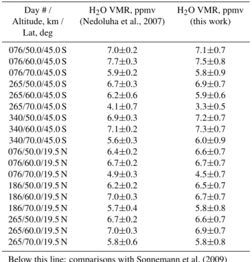
Table 5.Comparing H2O VMR retrieved from SABER with other measurements.

Day # / H₂O VMR, ppmv H₂O VMR, ppmv Altitude, km / (Nedoluha et al., 2007) (this work)

Lat, deg

076/50.0/45.0 S 7.0±0.2 7.1±0.7

076/60.0/45.0 S 7.7±0.3 7.5±0.8

076/70.0/45.0 S 5.9±0.2 5.8±0.9

265/50.0/45.0 S 6.7±0.3 6.9±0.7

265/60.0/45.0 S 6.2±0.6 5.9±0.6

265/70.0/45.0 S 4.1±0.7 3.3±0.5

340/50.0/45.0 S 6.9±0.3 7.2±0.7

340/60.0/45.0 S 7.1±0.2 7.3±0.7

340/70.0/45.0 S 5.6±0.3 6.0±0.9

076/50.0/19.5 N 6.4±0.2 6.6±0.7

076/60.0/19.5 N 6.7±0.2 6.7±0.7

076/70.0/19.5 N 4.9±0.3 4.5±0.7

186/50.0/19.5 N 6.2±0.2 6.5±0.7

186/60.0/19.5 N 7.0±0.3 6.7±0.7

186/70.0/19.5 N 5.7±0.4 5.8±0.8

265/50.0/19.5 N 6.7±0.2 6.6±0.7

265/60.0/19.5 N 7.0±0.3 6.9±0.7

265/70.0/19.5 N 5.8±0.6 5.8±0.8

Below this line: comparisons with Sonnemann et al. (2009)

076/50.0/69.2 N 4.5±0.3 4.5±0.5

076/60.0/69.2 N 4.0±0.3 3.7±0.4

076/70.0/69.2 N 2.2±0.2 2.6±0.4

076/80.0/69.2 N 1.4±0.2 1.6±0.4

186/50.0/69.2 N 7.0±0.5 6.2±0.6

186/60.0/69.2 N 6.5±0.5 6.0±0.6

186/70.0/69.2 N 6.7±0.6 5.7±0.8

186/80.0/69.2 N 3.6±0.6 4.5±1.0

265/50.0/69.2 N 7.5±0.5 6.5±0.6

265/60.0/69.2 N 6.5±0.7 6.0±0.6

265/70.0/69.2 N 5.0±0.6 4.7±0.6

265/80.0/69.2 N 2.5±0.5 3.0±0.6

SABER H2O VMR retrievals shows a good agreement with other measurements taking into account the accuracy of the compared data.

6.2.2 Meridional structure

The retrieved SABER water vapor distribution in Fig. 8a–h follows a known latitudinal pattern for seasons considered here. The H2O VMR decreases from the summer to the win-ter hemisphere is clearly seen in Fig. 8d, h and, to a lesser extent, in Fig. 8b, f. This is explained by changes in verti-cal wind during different seasons: the downward transport is increased in winter, but changes to the upward transport in summer (Garcia and Solomon, 1994; K¨orner and Sonne-mann, 2001). As a result, in winter the air from above, where

the H2O VMRs are small due to the mesospheric photochem-ical effects, moves down hence drying the atmosphere. The summertime mechanism works in the opposite direction giv-ing rise to an increased H2O VMR in mesosphere. Another reason for the H2O VMR decrease from the summer to the winter hemisphere is the strong pressure decrease at high lat-itudes in the winter hemisphere that is linked with the lower temperatures below∼70 km altitude.

The small-scale latitudinal structures that can be seen on nearly all panels of Fig. 8 can be explained by a strong ver-tical wind variability discussed by K¨orner and Sonnemann (2001). Their Fig. 5b shows that wind direction changes 6 times as the latitude varies from 60◦S to 60◦N leading to horizontal inhomogeneities in the H2O mixing ratio distribu-tions. The differences between vernal equinoxes of 2004 and 2007 (Fig. 8a and e, respectively) can be explained by larger downward transport at high latitudes in 2007 that is seen as an abrupt change in H2O VMR decrease at 30◦N. The same trend is seen on Fig. 8f where well-defined horizontal struc-tures reveal strong vertical wind variability, while low H2O VMR values at 10◦S indicate the direction of vertical winds in this area. Larger peak values at heights around 60 km in 2007 can be explained both by larger vertical wind activity and photochemical effects. Generally, this maximum arises due to a competition of two photochemical processes: pho-todissociation of H2O in the mesosphere and methane oxi-dation. The variations of solar activity have their maximum effect on H2O VMR at heights above 65 km (Chandra et al., 1997). Enhanced tropospheric CH4 emissions give rise to increased water vapor in the stratosphere and lower meso-sphere. One can explain the larger absolute values of H2O VMR in 2007 (Fig. 8e, g, and h) by a stronger vertical trans-port of methane from lower atmospheric layers. The com-prehensive analysis of the latitudinal and seasonal variations that will be possible with the coming new release of SABER data will reveal more information about these atmospheric phenomena.

7 From research to operational code

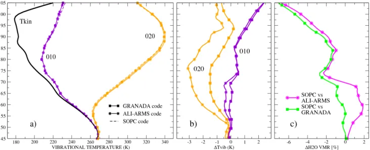
Fig. 9.Comparison of forward model for ALI-ARMS, GRANADA, and SOPC codes: (a)vibrational temperatures for 010 and 020 vibra-tional levels;(b)SOPC minus ALI-ARMS and SOPC minus GRANADA vibrational temperatures;(c)H2O VMR retrieval comparison: SOPC versus ALI-ARMS and GRANADA codes.

treated either line-by-line or by statistical band methods. For the calculations of the population of the water vapor vibra-tional levels shown here, the algorithm was set to use the lambda iteration technique (L´opez-Puertas and Taylor, 2001) and line-by-line treatment for solving the non-LTE problem. The GRANADA code has been used for the analysis of CO2, H2O, O3, CH4, NO2, NO, and CO emissions measured by the MIPAS instrument on the Envisat satellite (Fisher et al., 2008).

The SOPC non-LTE algorithm, based on the model devel-oped by L´opez-Puertas et al. (1995), uses the Curtis-matrix technique for the radiation transfer calculations (Goody and Young, 1995; L´opez-Puertas and Taylor, 2001). The vibra-tional level populations are found by solving a sequence of two-level problems starting from lower vibrational levels and moving towards the higher ones. The algorithm is iterative: the populations of all other vibrational levels that enter the balance equation for two selected levels are assumed to be known and updated by iterating the two-level problem se-quence. This algorithm was optimized for the SABER data processing (Mertens et al., 2001). The code uses the radia-tive transfer module described by Marshall et al. (1994) that replaces the computationally intensive line-by-line calcula-tions with pre-computed emissivity tables.

We compared the outputs of three codes using vertical profiles of atmospheric species retrieved from SABER mea-surements for different seasons as inputs. The water va-por VMR profiles were calculated with the LIMA model (Berger, 2008). For simplicity, the GRANADA and SOPC codes were not modified, and the comparisons were per-formed using the set of 7 vibrational levels, reaction rates from Table 1, and a fixed quantum yield for the O2(1) pump-ing (ε=4). Later on the SOPC will be modified to include

the new set of rates inferred from this work and the vertically varyingε profile. We believe that these modifications will not change the conclusions we present in this work and will not add to the estimated uncertainties in the SABER H2O VMR retrievals. Figure 9a shows the vibrational tempera-tures of the 010 and 020 levels calculated by three non-LTE codes. For this run we used the model atmosphere described in Sect. 3.1. The vibrational temperatures of the 010 level demonstrate a good agreement, differing by less than 1 K at altitudes below 95 km (Fig. 9a, b). The deviation for the sec-ond ν2 vibrational level (020) appears to be larger, reach-ing 3 K and 1.5 K at∼75 km altitude for the ALI-ARMS and GRANADA codes, respectively. These discrepancies in the vibrational temperatures correspond to∼2% and∼10% dif-ferences in the populations of the 010 and 020 levels, cor-respondingly, for the SOPC versus ALI-ARMS comparison. For the SOPC versus GRANADA comparison these values are∼2% and∼5% respectively. This corresponds to∼2% difference in the 6.6µm SABER filter bandpass radiances simulated by the operational and research codes. The differ-ences between H2O VMR values retrieved with the research and operational codes are shown in Fig. 9c. As one can see, they do not exceed 3% up to 90 km altitude and increase at higher altitudes. The latter increase does not affect the re-trievals below 90 km because of negligible H2O density at high altitudes.

8 Conclusion

We have described a non-LTE model and algorithm applied to the H2O VMR retrieval from the 6.6µm emissions mea-sured by SABER. The numerical experiments showed that the retrieval method provides a stable solution that does not depend on the initial guess profile. The SABER operational code was validated against two research non-LTE codes, and the differences in the simulated radiances at altitudes up to 90 km were less than 3%.

We have analyzed the sensitivity of H2O VMR retrievals to the rate coefficients used in the non-LTE modeling and inferred the deficiencies of the models for the interpretation of the broadband 6.6µm non-LTE emission developed by L´opez-Puertas et al. (1995) and Manuilova et al. (2001). Using the coincident H2O density measurements performed by the ACE-FTS occultation instrument, we have found new values for three rates that affect the H2O(ν2)populations and have recommended an update to the H2O non-LTE model: k∗_V−V{1}(H2O–O2)=(1.2+0.4/−0.1)×10−12cm3s−1; k∗_V−T{2}(O2–O)=(3.3±0.7)×10−12cm3s−1;

k∗_V−T{7,8}(H2O–M)=(1.4±0.4)×kV−T{7,8}(H2O–M). Performing the retrievals with the updated model produces the H2O VMR distributions similar to those measured by other instruments and predicted by models. The absolute H2O VMR values retrieved from SABER at 50.0–85.0 km altitudes were compared to MLS, HALOE, WVMS, and mi-crowave measurements at 45.0◦S, 19.5◦N, and 69.2◦N, and the agreement was good – within the experimental uncertain-ties of the datasets.

Qualitatively, the latitudinal distribution of SABER H2O VMR profiles calculated for four seasons in 2004 and 2007 agrees with climatology. It demonstrates the main features typical for the water vapor distribution in the middle and upper atmosphere: an increase of the H2O VMR from the winter hemisphere to the summer hemisphere and the circu-lation cells in the equatorial and middle latitude regions that are consistent with current understanding of the physics of the region. The approach developed in this work makes it possible to retrieve H2O VMR spatial and temporal distribu-tions for the entire SABER mission (∼2×106profiles) from 25 January 2002 until present. In the future, we plan to ex-tend the retrieval algorithm to include the nighttime measure-ments. This will double the number of H2O VMR profiles retrieved from SABER and enhance the utility of the dataset.

Appendix A

Abbreviations

ACE Atmospheric Chemistry Experiment ALI-ARMS Accelerated Lambda Iterations for

At-mospheric Radiation and Molecular Spectra

ALOMAR Arctic Lidar Observatory for Middle Atmosphere Research

ASTRO-SPAS Astronomical Shuttle-Pallet Satellite ATMOS Atmospheric Trace MOlecule

Spec-troscopy

BANDPAK software PAcKage for calculating the radiative transfer in BANDs

CRISTA Cryogenic Infrared Spectrometers and Telescopes for the Atmosphere, the instrument on board of the ASTRO-SPAS satellite

FTS Fourier-Transform Spectrometer GRANADA Generic RAdiative traNsfer AnD

non-LTE population Algorithm

HALOE HALogen Occultation Experiment on board of the UARS satellite

HITRAN HIgh-resolution TRANsmission molecular absorption database

KOPRA Karlsruhe Optimized and Precise Ra-diative transfer Algorithm

LIMA Leibniz-Institute Middle Atmosphere LIMS Limb Infrared Monitor of the

Strato-sphere

LTE Local Thermodynamic Equilibrium MIPAS Michelson Interferometer for Passive

Atmospheric Sounding

MLT Mesosphere/Lower Thermosphere

NLC Noctilucent Cloud

PMSE Polar Mesospheric Summer Echoe

RT Radiative Transfer

SABER Sounding of the Atmosphere using Broadband Emission Radiometry SAMS the Stratospheric And Mesospheric

Sounder

SCISAT1 SCIence SATellite 1 SMR Sub-Millimeter Radiometer SNR Signal to Noise Ratio

SOFIE Solar Occultation for Ice Experiment

SOPC SABER Operational Code

TIMED Thermosphere Ionosphere Mesosphere Energetics and Dynamics

UARS Upper Atmosphere Research Satellite

VMR Volume Mixing Ratio

Acknowledgements. This research was supported by NASA grant NNX08AG41G. This work was also partially supported by Spanish MICINN under contract AYA2008-03498/ESP and EC FEDER funds. SABER V1.07 atmospheric data were downloaded from the http://saber.gats-inc.com/ Web site. The authors are grateful to the SABER science, data processing, and flight operations for their ongoing support of this work. The authors also want to thank Gerd Sonnemann and Uwe Berger from the Leibniz Institute for Atmospheric Physics, K¨uhlungsborn, Germany for the fruitful discussions and assistance in this work. The Atmospheric Chemistry Experiment is a Canadian-led mission mainly supported by the Canadian Space Agency (CSA) and the Natural Sciences and Engineering Research Council of Canada (NSERC). ACE-FTS data were provided by the European Space Agency.

Edited by: W. Ward

References

Barnet, J. J.: Satellite-borne measurements of middle-atmosphere temperature, Phil. Trans. R. Soc. London, A, 323, 527–544, 1987.

Bass, H. E.: Vibrational relaxation in CO2/O2mixtures, J. Chem. Phys., 58(11), 4783–4786, 1973.

Bass, H. E. and Shields, F. D.: Vibrational relaxation and sound ab-sorption in O₂/H₂O mixtures, J. Acoust. Soc. Am., 56(3), 856– 859, 1974.

Bass, H. E., Keeton, R. G., and Williams, D.: Vibrational and ro-tational relaxation in mixtures of water vapor and oxygen, J. Acoust. Soc. Am., 60(1), 74–77, 1976.

Bass, H. E.: Absorption of sound by air: high temperature predic-tions, J. Acoust. Soc. Am., 69, 124–138, 1981.

Berger, U.: Modeling of middle atmosphere dynamics with LIMA, J. Atmos. Solar-Terr. Phy., 1170–1200, doi:10.1016/j.jastp.2008.02.004, 2008.

Bernath, P. F., McElroy, C. T., Abrams, M. C., Boone, C. D., Butler, M., Camy-Peyret, C., Carleer, M., Clerbaux, C., Coheur, P. F., Colin, R., DeCola, P., DeMazi`ere, M., Drummond, J. R., Dufour, D., Evans, W. F. J., Fast, H., Fussen, D., Gilbert, K., Jennings, D. E., Llewellyn, E. J., Lowe, R. P., Mahieu, E., McConnell, J. C., McHugh, M., McLeod, S. D., Michaud, R., Midwinter, C., Nas-sar, R., Nichitiu, F., Nowlan, C., Rinsland, C. P., Rochon, Y. J., Rowlands, N., Semeniuk, K., Simon, P., Skelton, R., Sloan, J. J., Soucy, M.-A., Strong, K., Tremblay, P., Turnbull, D., Walker, K. A., Walkty, I., Wardle, D. A., Wehrle, V., Zander, R., and Zou, J.: Atmospheric Chemistry Experiment (ACE): Mission overview, Geophys. Res. Lett., 32, L15S01, doi:10.1029/2005GL022386, 2005.

Bevilacqua, R. M., Schwartz, P. R., Bologna, J. M., Thacker, D. J., Olivero, J. J., and Gibbins, C. J.: An observational study of water vapor in the mid-latitude mesosphere using ground-based microwave techniques, J. Geophys. Res., 88, 8523–8534, 1983. Boone, C. D., Nassar, R., Walker, K. A., Rochon, Y., McLeod, S. D.,

Rinsland, C. P., and Bernath, P. F.: Retrievals for the atmospheric chemistry experiment Fourier-transform spectrometer, Appl. Op-tics, 44(33), 7218–7231, 2005.

Boone, C. D., Walker, K. A., and Bernath, P. F.: Speed-dependent Voigt profile for water vapor in infrared remote sensing applica-tions, J. Quant. Spectrosc. Ra., 105, 525–532, 2007.

Brasseur, G. P. and Solomon, S.: Aeronomy of the middle atmo-sphere, Springer, 644 pp, 2005.

Breen, J. E., Quy, R. B., and Glass, G. P.: Vibrational relaxation of O2 in the presence of atomic oxygen, J. Chem. Phys., 59, 556– 557, 1973.

Carleer, M. R., Boone, C. D., Walker, K. A., Bernath, P. F., Strong, K., Sica, R. J., Randall, C. E., V¨omel, H., Kar, J., H¨opfner, M., Milz, M., von Clarmann, T., Kivi, R., Valverde-Canossa, J., Sioris, C. E., Izawa, M. R. M., Dupuy, E., McElroy, C. T., Drummond, J. R., Nowlan, C. R., Zou, J., Nichitiu, F., Lossow, S., Urban, J., Murtagh, D., and Dufour, D. G.: Validation of wa-ter vapour profiles from the Atmospheric Chemistry Experiment (ACE), Atmos. Chem. Phys. Discuss., 8, 4499–4559, 2008, http://www.atmos-chem-phys-discuss.net/8/4499/2008/. Chandra, S., Jackman, C. H., Fleming, E. L., and Russell III, J. M.:

The seasonal and long-term changes in mesospheric water vapor, Geophys. Res. Lett., 24(6), 639–642, 1997.

Copeland, R. A.: Measurement of oxygen vibrational relaxation rate constant with oxygen atoms at low temperature, SRI Project P18443, Monthly Report MP 08-067, 2008.

Croom, D. L., Gibbins, C. J., Birks, A. R., and Wrench, C. L.: Ground-based remote sensing of atmospheric H2O in the 25– 100 km region of the atmosphere, in: Union Radio Scientifique Internationale, Open Symposium, La Baule, Loire-Atlantique, France, 28 April–6 May 1977, Proceedings, A78-25801 09-32 Issy-les-Moulineaux, Hauts-de-Seine, France, Comite National Francais de la Radio-electricite Scientifique, 547–550, 1977. Diskin, G. S., Lempert, W. R., and Miles, R. B.: Observation of

vibrational dynamics in X36−g-oxygen following stimulated Ra-man excitation to the v=1 level: implications for the RELIEF flow tagging technique; AIAA 96-3001, 34-th Aerospace Sci-ences Meeting and Exhibit: Reno, NV, 15–18 January 1996. Drummond, J. R., Houghton, J. T., Peskett, G. D., Rodgers, C. D.,

Wale, M. J., Whitney, J., and Williamson, E. J.: The Strato-spheric and MesoStrato-spheric Sounder on Nimbus 7, Philosophical Transactions of the Royal Society of London, Series A, Math-ematical and Physical Sciences, 296(1418), The Middle Atmo-sphere as Observed form Balloons, Rockets and Satellites, 219– 241, 1980.

Edwards, D. P., Kumer, J. B., L´opez-Puertas, M., Mlynczak, M. G., Gopalan, A., Gille, J. C., and Roche, A.: Non-local thermody-namic equilibrium limb radiance near 10µm as measured by UARS CLAES, J. Geophys. Res., 101(D21) 26577–26588, 1996. Edwards, D. P., Zaragoza, G., Riese, M., and L´opez-Puertas, M.: Evidence of H2O nonlocal thermodynamic equilibrium emission near 6.4µm as measured by cryogenic infrared spectrometers and telescopes for the atmosphere (CRISTA 1), J. Geophys. Res., 105(D23), 29003–29021, 2000.

Esposito, F. and Capitelli, M.: The relaxation of vibrationally ex-cited O2molecules by atomic oxygen, Chem. Phys. Lett., 443, 222–226, 2007.

Finzi, J., Hovis, F. E., Panfilov, V. N., Hess, P., and Moore, C. B.: Vibrational relaxation of water vapor, J. Chem. Phys., 67(9), 4053–4061, 1977.