www.atmos-chem-phys.net/14/8269/2014/ doi:10.5194/acp-14-8269-2014
© Author(s) 2014. CC Attribution 3.0 License.
CarbonTracker-CH
4
: an assimilation system for estimating
emissions of atmospheric methane
L. Bruhwiler1, E. Dlugokencky1, K. Masarie1, M. Ishizawa2, A. Andrews1, J. Miller1,4, C. Sweeney1,4, P. Tans1, and D. Worthy3
1NOAA Earth System Research Laboratory, Global Monitoring Division, Boulder Colorado, USA 2National Institute for Environmental Studies, Center for Global Environmental Research, Tsukuba, Japan 3Environment Canada, Climate Research Division, Toronto, Ontario, Canada
4Cooperative Institute for Research in Environmental Sciences, University of Colorado, Boulder, Colorado, USA
Correspondence to:L. M. Bruhwiler ([email protected])
Received: 18 October 2013 – Published in Atmos. Chem. Phys. Discuss.: 24 January 2014 Revised: 22 June 2014 – Accepted: 23 June 2014 – Published: 19 August 2014
Abstract. We describe an assimilation system for atmo-spheric methane (CH4), CarbonTracker-CH4, and
demon-strate the diagnostic value of global or zonally averaged CH4 abundances for evaluating the results. We show that
CarbonTracker-CH4 is able to simulate the observed zonal
average mole fractions and capture inter-annual variability in emissions quite well at high northern latitudes (53–90◦N). In contrast, CarbonTracker-CH4is less successful in the
trop-ics where there are few observations and therefore misses significant variability and is more influenced by prior flux estimates. CarbonTracker-CH4 estimates of total fluxes at
high northern latitudes are about 81±7 Tg CH4yr−1, about 12 Tg CH4yr−1 (13 %) lower than prior estimates, a result
that is consistent with other atmospheric inversions. Emis-sions from European wetlands are decreased by 30 %, a result consistent with previous work by Bergamaschi et al. (2005); however, unlike their results, emissions from wetlands in boreal Eurasia are increased relative to the prior estimate. Although CarbonTracker-CH4does not estimate an
increas-ing trend in emissions from high northern latitudes for 2000 through 2010, significant inter-annual variability in high northern latitude fluxes is recovered. Exceptionally warm growing season temperatures in the Arctic occurred in 2007, a year that was also anonymously wet. Estimated emissions from natural sources were greater than the decadal average by 4.4±3.8 Tg CH4yr−1in 2007.
CarbonTracker-CH4estimates for temperate latitudes are
only slightly increased over prior estimates, but about 10 Tg CH4yr−1is redistributed from Asia to North America.
This difference exceeds the estimated uncertainty for North America (±3.5 Tg CH4yr−1). We used time invariant prior flux estimates, so for the period from 2000 to 2006, when the growth rate of global atmospheric CH4was very small,
the assimilation does not produce increases in natural or an-thropogenic emissions in contrast to bottom-up emission data sets. After 2006, when atmospheric CH4began its recent
in-creases, CarbonTracker-CH4allocates some of the increases
to anthropogenic emissions at temperate latitudes, and some to tropical wetland emissions. For temperate North America the prior flux increases by about 4 Tg CH4yr−1during
win-ter when biogenic emissions are small. Examination of the residuals at some North American observation sites suggests that increased gas and oil exploration may play a role since sites near fossil fuel production are particularly hard for the inversion to fit and the prior flux estimates at these sites are apparently lower and lower over time than what the atmo-spheric measurements imply.
The tropics are not currently well resolved by CarbonTracker-CH4 due to sparse observational
cover-age and a short assimilation window. However, there is a small uncertainty reduction and posterior emissions are about 18 % higher than prior estimates. Most of this increase is allocated to tropical South America rather than being distributed among the global tropics. Our estimates for this source region are about 32±4 Tg CH4yr−1, in good
agreement with the analysis of Melack et al. (2004) who obtained 29 Tg CH4yr−1for the most productive region, the
1 Introduction
Methane (CH4) is second in importance to carbon
diox-ide (CO2) among greenhouse gases with significant
anthropogenic sources. It has a radiative forcing of, 0.5±0.05 Wm−2, about 28 % that of non-CO2atmospheric constituents in 2010 (Hofmann et al., 2006; updated at http: //www.esrl.noaa.gov/gmd/aggi/). Over a 100 yr time horizon CH4is 28 times more efficient per mass as a greenhouse gas
than CO2(Myhre et al., 2013).
Global emissions of CH4 are between 500 and
600 Tg CH4yr−1 (Kirschke et al., 2013 and this work)
and about 40 % of this is due to natural sources, mainly wetlands. The other 60 % of global emissions are due to microbial emissions associated with rice agriculture, livestock and waste, and fugitive emissions from fossil fuel production and use (Denman et al., 2007). Global emissions have recently been approximately in balance with global sinks, mainly chemical destruction by reaction with OH, but also from oxidation by soil microbes, and atmospheric reactions with O1D and Cl in the stratosphere. The lifetime of CH4in the atmosphere is about 10 yr (e.g., Dlugokencky
et al., 2003) with CO2the eventual product of its oxidation.
CH4 has increased from a preindustrial abundance of
722±4 ppb (Etheridge et al., 1998 after conversion to the NOAA 2004 CH4standard scale, Dlugokencky et al., 2005)
to current values of about 1800 ppb in 2010 (about 2.5 times), and it is likely that human activity is responsible for most of this increase. Current levels are unprecedented over at least the last 800 kyr (Loulerge et al., 2008). NOAA atmospheric network observations extend back to the 1980s, and show that global CH4 increased rapidly through the late 1990s,
leveled off during the early 2000s and have recently begun to increase since 2007 (Rigby et al., 2008; Dlugokencky et al., 2009). The subject of the causes of the recent increase is the topic of much recent work (e.g., Bousquet et al., 2011), including this study.
An important aspect of atmospheric CH4 is the
sensitiv-ity of natural wetland emissions to climate change. Emis-sions from the Arctic, in particular, have the potential to in-crease significantly as temperatures rise and the vast stores of soil carbon thaw (e.g., Schuur et al., 2011; Harden et al., 2012). Schaefer et al. (2011) pointed out that potential car-bon emissions from the Arctic could have important implica-tions for policies aimed at reducing or stabilizing emissions. This clearly highlights the importance of maintaining long-term measurements of atmospheric CH4 in the Arctic, and
in this study we hope to further the case for atmospheric in-verse techniques as a tool to diagnose observed atmospheric records (see previous studies by Hein et al., 1997; Houwel-ing et al., 1999, 2013; Chen and Prinn, 2006; Bergamaschi et al., 2005, 2014; Bousquet et al., 2006).
Atmospheric CH4is also influenced by diverse human
ac-tivities, ranging from food production (ruminants and rice) to waste (sewage and landfills) to fossil fuel production (coal,
oil and gas). Future increases in population could increase emissions from agriculture and waste as demand for more food production rises, while the current boom in shale oil/gas exploitation has focused attention on leakage from drilling, storage and transport of fossil fuel (e.g., Pétron et al., 2012). An obvious use of an atmospheric assimilation system is to quantify changes in anthropogenic emissions and attribute increases at policy relevant spatial scales, something that is possible only with adequate spatial coverage of observations. In this study we will discuss the degree to which this is cur-rently possible given the coverage of the current observa-tional network.
The work we present here uses only surface observa-tions rather than combinaobserva-tions of surface observaobserva-tions and retrievals space-based instruments as used by Bergamaschi et al. (2013) and Houweling et al. (2014). Our study differs from that of Bergamaschi et al. (2013) since they used a sub-set of 30 surface observations sampling mainly background marine air that existed over the entire decade, as well as satel-lite retrievals. In our study we have used most available sur-face observations, including those that are sensitive to terres-trial emissions (Table 2). We use the same transport model as Bergamaschi et al. (2013) and Houweling et al. (2014), how-ever, we use a different assimilation technique and different strategies for weighting observations and priors. We also in-clude a discussion of observationally derived quantities that useful evaluation of our results.
The next section is a detailed description of our CH4
as-similation system, CarbonTracker-CH4, followed by a
de-tailed evaluation of its performance. In Sect. 4, we discuss results from CarbonTracker-CH4for 2000–2010.
2 The CarbonTracker ensemble data assimilation system
The total emission of CH4 in time and space may be
de-scribed by
F (x, y, t )=λ1·Fnatural(x, y, t )+λ2·Ffossil(x, y, t )+λ3
·Fagriculture/waste(x, y, t )+λ4·Ffire(x, y, t )+λ5
·Focean(x, y, t ),
whereλi represents a set of linear scaling factors to be
es-timated in the assimilation that are applied to the fluxes (F) by multiplying prior estimates of CH4fluxes to produce the
Figure 1. Map showing locations of observations used in CarbonTracker-CH4. Shading indicates the boundaries of the Transcom 3 source regions (Gurney et al., 2000) with an additional tropical African region.
include fugitive emissions from coal, oil and gas production (estimated as one source); agriculture and waste emissions (rice production, for example); livestock and their waste; and emissions from landfills and waste water. Natural emissions include contributions from wetlands, termites, uptake in soils and wild animals. The final terrestrial emission category is biomass burning, which is treated as a separate category due to the existence of strong spatial constraints coming from satellite observations of locations of large fires. In general, the spatial distribution of the prior flux estimates is an impor-tant constraint on the assimilation. For example, the known location of fossil fuel production from bottom-up emission data sets provides information pertaining to the assimilation system on whether a signal measured at a particular obser-vation site could have a fossil fuel component. If production areas change over time and are not captured by the prior dis-tribution, then fossil fuels will be underestimated by the in-version.
In this study we estimate emissions for continental scale source regions, and although we rely on the prior spatial distribution of the prior emissions to distribute the emis-sions, the use of large source regions can lead to aggrega-tion errors as shown by Kaminski et al. (2001). An alter-native would be to solve for many more sources, possibly at grid scale. However, without significantly more observa-tional constraints, our solution would be very dependent on not only the prior emissions, but also their assumed spatial and temporal covariance. Ultimately, use of space-based ob-servations might be the preferred solution. At present, sig-nificant issues with space-based emissions still exist, such as quantification of biases that vary with space and time (e.g., Houweling et al., 2013). On the other hand, as discussed by Bruhwiler et al. (2011), the global network can constrain cer-tain aspects of the budgets of greenhouse gases, even with its bias towards background atmospheric sites.
We initialized the assimilation using an equilibrated dis-tribution produced by a previous TM5 run that was scaled to match observed zonal average CH4mixing ratio for the year
2000. The north–south gradient therefore should represent the observed atmospheric gradient at the surface. Sensitivity runs using synthetic data (not shown) suggest that spin-up effects are restricted to within in the first half year of the as-similation.
2.1 Ensemble size and localization
The ensemble Kalman smoother system used to solve for the scalar multiplication factors is based on that described by Peters et al. (2005), and uses the square root ensemble Kalman filter of Whitaker and Hamill (2002). The length of the smoother window is restricted to 5 weeks for computa-tional efficiency. Although the posterior flux estimates in rel-atively densely sampled regions such as North America were found to be robust by Peters et al. (2005) with a window this short, regions with less dense observational coverage (the tropics, for example) are likely to be poorly constrained even after more than a month of transport and therefore not well resolved. As pointed out by Bruhwiler et al. (2005), a smoother window of at least 3 months is likely to make max-imal use of remote network sites, however this may come at the expense of accumulated errors in transport as claimed by Peters et al. (2007). The extent to which this is true is a subject for further study. Even without the problem of a short smoother window, the sparseness of the observational network makes it difficult to resolve under-sampled regions such as the tropical terrestrial biosphere (Bruhwiler et al., 2011).
Statistics for the ensemble are created from 500 members using the prior covariance matrix of the parameters, each with its own background CH4 concentration field to
repre-sent the time history (and thus covariances) of the filter. We experimented with different numbers of ensemble members and found that the use of too few ensemble members results in solutions that stay artificially close to prior flux estimates. To dampen spurious noise due to the approximation of the covariance matrix, we apply localization (Houtekamer and Mitchell, 1998) for non-background sites. By limiting cor-relations between distant sites, localization ensures that ran-dom correlations between parameters do not translate into unrealistic constraints on emissions by distant measurement sites (i.e., those connections physically impossible with only 5 weeks of transport). Following Peters et al. (2005) local-ization is based on the linear correlation coefficient between the 500-parameter deviations and 500 observation deviations for each parameter, with a cut-off at 95 % significance in a student’sttest with a two-tailed probability distribution.
as annual uncertainties will likely be overestimates since in-formation about temporal covariations will be limited. Fur-thermore, as with any inversion, the error covariance matrix ultimately reflects the relative weighting between the model– data mismatch errors and prior emission uncertainties that are specified.
2.2 Covariance structure
In our assimilation, the chosen 1-s error of the prior estimates is 75 % for all parameters. The prior covariance structure de-scribes the uncertainty on each parameter, plus their correla-tion in space. For the current version of CarbonTracker-CH4,
we assumed a diagonal prior covariance matrix so that no prior correlations between estimated parameters exist. The effect of this choice may be strong anti-correlations among estimated parameters in regions where few observational constraints exist; however, larger-scale aggregations of these regions are expected to yield more robust estimates. For ex-ample, the total tropical source can be better determined that the individual regions between which there can be trade-offs in emissions from time step to time step. Note also that the 5-week assimilation window used by CarbonTracker limits knowledge of temporal correlations. As a result, the uncer-tainty on annual average emissions is difficult to estimate.
2.3 TM5 atmospheric transport model
Transport Model 5 (TM5, Krol et al., 2005) is a commu-nity supported global model with two-way nested grids. For CarbonTracker-CH4, we ran the simulation at 4◦latitude×
6◦longitude resolution without zoom regions. TM5 is devel-oped and maintained jointly by the Institute for Marine and Atmospheric Research Utrecht (IMAU, the Netherlands), the Joint Research Centre (JRC, Italy), the Royal Netherlands Meteorological Institute (KNMI, the Netherlands), and the National Oceanic & Atmospheric Administration (NOAA) Earth System Research Laboratory (ESRL, USA). TM5 has detailed treatments of advection, convection (deep and shal-low), and vertical diffusion in the planetary boundary layer and free troposphere. The winds used for transport in TM5 come from the European Center for Medium range Weather Forecast (ECMWF) operational forecast model. This “par-ent” model currently runs with∼25 km horizontal resolution and 60 layers in the vertical prior to 2006 and 91 layers in the vertical from 2006 onwards.
The ECMWF meteorological data are preprocessed into coarser grids and are converted from wind fields to mass con-serving horizontal and vertical mass fluxes. TM5 runs at an external time step of 3 hours, but due to the symmetrical op-erator splitting between advection, diffusion, emissions and loss the effective time step over which each process is ap-plied is shorter. The vertical resolution of TM5 used with CarbonTracker-CH4is 34 hybrid sigma-pressure levels (from
2006 onwards; 25 levels for 2000–2005), unevenly spaced
with more levels near the surface. At the time the calcula-tions discussed in this study were done, we did not have the ERA-Interim reanalysis driving meteorology and older re-analyses did not cover the time span we were interested in. Comparisons of forward simulations suggest that differences between ERA-I and OD for CH4at surface sites is very small,
both before and after the change in the vertical levels. Assim-ilations run with both data products for CarbonTracker (CO2)
produce virtually indistinguishable results in estimated fluxes (see http://www.esrl.noaa.gov/gmd/ccgg/carbontracker/).
As noted by Peters et al. (2004), TM5 overestimates the meridional gradient of SF6by about 20 %. A systematic
com-parison of a suite of transport models described by Den-ning et al. (1999) found that some transport models appear to underestimate mixing processes, especially near the sur-face, while others mix emissions more rapidly throughout the lower atmosphere. They also found that models that underes-timate mixing produce relatively good simulations of marine boundary layer sites while overestimating concentrations at continental sites. More diffusive models produced worse ma-rine boundary layer simulations, but did better for continental sites. TM5 falls into less-diffusive category, but current ongo-ing development is aimed at improvongo-ing the situation. It must be acknowledged that the emissions estimates in our study may be biased due to inadequate vertical mixing. For exam-ple, more vertical mixing will diffuse emissions throughout a deeper atmospheric column, and this may result in higher emissions in order to match observations.
2.4 Prior emission estimates for natural sources
The largest natural emissions of methane are from wetlands, defined as regions that are permanently or seasonally wa-ter logged. Wetlands are a broad category that includes both high-latitude bogs and fens and tropical swamps. Saturated soils in warm tropical environments tend to produce the most methane. However, warming Arctic temperatures raise con-cerns of increasing output from high-latitude wetlands and future decomposition of carbon currently stored in frozen Arctic soils (e.g., Schaefer et al., 2011).
Methane is rapidly oxidized by methanotrophic bacteria in overlying aerobic water columns or unsaturated soil, so the water table must be at or near the surface and the depth of overlying water must be shallow for large emissions to occur. Wetland plants have adapted to low oxygen environments by having hollow stems to allow delivery of oxygen and other gases to root systems. These hollow stems also allow deliv-ery of methane directly to the atmosphere, and along with ebullition account for most of transport to the atmosphere. Diffusion also occurs but is a significantly smaller contribu-tion to the atmosphere. (See Barlett and Harris (1993) for an extensive overview of wetland emissions.) Bottom-up es-timates of global emissions from wetlands are about 150– 200 Tg CH4yr−1with most of this occurring in tropical
to temperature and precipitation, they exhibit significant sea-sonal cycles, especially at high latitudes, as well as inter-annual variability due to moisture and temperature variabil-ity.
Methane emissions from wetlands are difficult to quantify using assimilation systems for two reasons; their global spa-tial distribution is difficult to know accurately, and there is large variability in emission rates over small spatial scales (meters), which makes extrapolation to large scales diffi-cult. Here we used the prior flux estimates of Bergamaschi et al. (2005) that are based on the wetland distribution of Matthews (1989) and the wetland emission model of Kaplan (2002) that parameterizes emissions based on moisture, tem-perature and soil carbon. The global total of the prior flux estimate is 175 Tg CH4yr−1.
Other natural sources of methane include enteric fermen-tation in insects (mainly termites, Sanderson, 1996) and wild ruminants (Houweling et al., 1999). Prior values for both of these sources (∼25 Tg CH4yr−1)are much smaller than the wetland source. Oxidation of CH4 in dry soils
(∼40 Tg CH4yr−1, Ridgwell et al., 1999) is a natural sink of CH4and is treated as a negative source in the assimilation.
2.5 Prior emission estimates for fugitive emissions from fossil fuels
Methane is the principal component of natural gas, and leaks to the atmosphere associated with natural gas production and distribution are a considerable source. Natural gas is as-sociated with oil production and is often flared, or simply vented to the atmosphere. Together, anthropogenic emissions from oil and gas production are thought to contribute about 50 Tg CH4yr−1(∼10 % of the global annual methane
emis-sions, EDGAR 3.2FT2000 (European Commission, JRC, 2009). Methane is also associated with coal deposits and can be released by extracting and pulverizing coal. It is of-ten vented directly to the atmosphere from mines, and this source contributes an additional∼20 Tg CH4yr−1(EDGAR 3.2FT2000 (European Commission, JRC, 2009). As Asian economies have undergone rapid growth, coal production there has increased by a factor of about two since 2000, while remaining approximately level for most of the rest of the world. In 2010, production of coal by China increased by 9 % over the previous year (BP Statistical Energy Review, 2011). Combustion of natural gas is currently used to generate about a quarter of the electricity produced in the US. Its pop-ularity as a fuel has recently grown because it is a relatively clean and efficient source of energy. Recent technological advances in recovery of natural gas, principally hydraulic fracturing, have led to increases in reserve estimates, and a tremendous increase in exploitation of shale oil/gas deposits in North America (e.g., Energy Information Administration; http://www.eia.gov). It is possible that as natural gas reserves are increasingly exploited, emissions related to its production and distribution will rise in the future.
CarbonTracker-CH4 uses the 1◦×1◦ gridded emissions
from EDGAR 3.2FT2000 (European Commission, JRC, 2009) as prior emission estimates for fugitive emissions from coal, oil and gas production. This data set is based on emis-sion inventories by country and sector for 1990 and 1995 ex-trapolated to 2000 using production and consumption statis-tics. We have not extrapolated this data over the period cov-ered by CarbonTracker-CH4, and have instead kept prior
emission estimates constant at 2000 levels. This will allow us to test whether the emission estimates suggest changes in anthropogenic emissions, for example, the large increase in emissions from coal production in Asia or the significant in-crease in oil and gas drilling over the last decade in North America. In some cases, the spatial distributions of priors may not be accurate since they may be based on simple as-sumptions like population. For other emissions, there may have been changes in the spatial distribution of emissions over the decade, oil and gas drilling in North America for example. The atmospheric inversions allow the possibility of diagnosing these problems in the underlying prior emission data sets and may lead to improvements in methodology.
2.6 Prior emission estimates for agriculture and waste
The largest source of methane emitted by human activity is agriculture and waste; emissions from rice agriculture, waste/wastewater, and animals and their waste total 230– 250 Tg CH4yr−1. Ruminants, such as cattle, goats, sheep and
water buffalo are able to convert hard-to-digest forage to en-ergy through enteric fermentation, in which microbes pro-duce easily digested material inside the animal’s gut. Emis-sions from enteric fermentation may be expected to increase with increasing human population and higher standards of living. Animal waste, along with waste water and landfills produce CH4 when conditions favor anaerobic
decomposi-tion. Organic material is decomposed in low oxygen condi-tions by chains of microbial processes that terminate in pro-duction of methane by methanogens.
Rice agriculture is also a significant source of methane to the atmosphere. This is because warm, waterlogged organic-rich soils in rice paddies are ideal for methanogenesis. Bottom-up estimates of emissions from rice agriculture are 50 Tg CH4yr−1, and emissions can be significantly reduced
by drainage of paddies between harvests as well as other agri-cultural practices (Yan et al., 2009).
CarbonTracker-CH4 uses the 1◦×1◦ gridded emissions
have instead kept prior emission estimates constant at 2000 levels as for fossil fuel emissions.
2.7 Prior emission estimates for biomass burning
Fires are a relatively small part of the atmospheric CH4
bud-get: 15–20 Tg CH4yr−1out of a total of∼520 Tg CH4yr−1,
however, they are an important contribution to inter-annual variability of methane.
The fire prior currently used in CarbonTracker-CH4 is
based on the Global Fire Emissions Database (GFED), which uses the CASA (Carnegie-Ames-Stanford Approach) bio-geochemical model to estimate the carbon fuel in various biomass pools along with burned area based on MODIS satellite observations of fire counts (Giglio et al., 2006; van der Werf et al., 2006). The data set consists of 1◦×1◦ gridded monthly burned area, fuel loads, combustion com-pleteness, and fire emissions for numerous atmospheric con-stituents, including CH4for the time period spanning January
1997–December 2010.
2.8 Prior estimates for ocean fluxes
The oceans play a relatively small role in the budget of atmospheric methane, contributing only ∼2–3 % of global emissions (∼10–15 Tg CH4yr−1). A significant fraction of this is assumed to come from methane seeps in shallow coastal waters (∼5 Tg CH4yr−1). The overlying water col-umn must be shallow for emission to the atmosphere, since CH4 is efficiently consumed by aerobic microbial
pro-cesses. The water column also needs to be shallow for bub-bles to deliver methane directly to the air. Coastal waters are sometimes supersaturated in CH4, and may emit about
6 Tg CH4yr−1 to the atmosphere, while the open may add
another 3 Tg CH4yr−1(Houweling et al., 1999; Lambert and
Schmidt, 1993).
Rhee et al. (2009) have suggested that global ocean emissions excluding natural seeps is much smaller than the ∼9 Tg CH4yr−1 we have used in this version of CarbonTracker-CH4, only about 0.6–1.2 Tg CH4yr−1. On
the other hand, recent studies conducted in the coastal waters of the eastern Siberian Arctic hint at the possibility of a sig-nificant source of methane coming from methane bubbling from the continental shelf sediments (Shakhova et al., 2010). For this version of CarbonTracker-CH4we followed the
ap-proach of Bergamaschi et al. (2009) and used the estimates of Houweling et al., (1999) and Lambert and Schmidt (1993) as prior flux estimates. We also assumed an uncertainty on these prior flux estimates of±75 %.
2.9 Atmospheric chemical loss
Methane is removed from the atmosphere mainly by reaction with hydroxyl radical (OH), but also by reaction with atomic chlorine (Cl) and excited-state oxygen (O1D) in the strato-sphere. The chemical loss of methane over a year is about
equal to the total input from sources (∼520 Tg CH4yr−1),
and the mean lifetime of methane is 9–10 yr. Small differ-ences in the emissions and losses lead to trends in atmo-spheric CH4 abundance, while year to year changes in the
balance of emissions and loss lead to inter-annual variability and possibly to trends in observed methane.
Hydroxyl radical is extremely reactive and has such a short atmospheric residence time that it is difficult to directly mea-sure its global distribution. Instead, observations of atmo-spheric species that have relatively well-quantified anthro-pogenic emissions and are destroyed only by reaction with OH, such as methyl chloroform (CH3CCl3), are used, often
along with atmospheric models, to estimate the abundance of atmospheric OH. Using an empirical approach, Montzka et al. (2011) noted that the inter-annual variability in atmo-spheric OH is likely to be within about∼2 %. Errors in de-rived OH distributions arise from uncertainty in the emis-sions of CH3CCl3used to estimate OH and uncertainties in
transport models. Krol et al. (1998) estimated that the uncer-tainty in globally averaged OH is±10 %.
About 10 % of total chemical loss is due to transport and chemical destruction in the stratosphere. A small amount of this methane-depleted air is returned to the troposphere and could influence interpretation of high-altitude (aircraft) measurements of methane. In addition, errors in simulating stratosphere-troposphere transport could result in biases for model simulations covering many years.
Errors in the chemical loss of methane and the inability to adequately resolve inter-annual variability of OH are trouble-some for estimation of methane fluxes. A 2 % variation in the global methane sink is equivalent to∼10 Tg CH4yr−1, about
the size of estimated inter-annual variability in methane emissions.
For the present version of CarbonTracker-CH4 we use
pre-calculated OH fields from a full-chemistry TM5 simu-lation that have been optimized against global observations of methyl chloroform. The chemical loss fields consist of a single, repeating seasonal cycle, and result in a methane life-time of about 9.5 yr. Details of the chemical loss fields may be found in Bergamaschi et al. (2005).
2.10 Observational constraints
This study uses measurements of air samples collected at surface sites in the NOAA ESRL Cooperative Global Air Sampling Network (http://www.esrl.noaa.gov/gmd/ccgg/ flask.html) except those identified as having analysis or sam-pling problems, or those thought to be strongly influenced by local sources. The availability of data varies over time. Data collection, quality control and analysis methods are described in detail by Dlugokencky et al. (1994). A map of sites used in CarbonTracker-CH4is shown in Fig. 1. In
addition, we use in situ quasi-continuous CH4 time series
Table 1.CarbonTracker-CH4data preprocessing.
Measurement Program
Data Preprocessing
ESRL discrete surface
All valid∗ data. Multiple values from the same day and location are averaged. No sample time-of-day restriction (see exception below).
EC in situ sites All valid data from highest intake. Day average using 12–16 LST.
∗In this context “Valid Data” means the observation is thought to be free of sampling and analytical problems and has not been influenced by local sources.
formerly Old Black Spruce), SK, Canada, 105 m a.g.l. at East Trout Lake, SK, Canada (ETL), 40 m a.g.l. at Fraserdale, ON, Canada (FRD), and 10 m a.g.l. at Lac Labiche, AB, Canada (LLB). Other in situ quasi-continuous CH4time series used
are from the EC Canadian sites at Alert, Nunavut (ALT), Sable Island, NS (SBL) and Egbert, ON (EGB). All observa-tions used in CarbonTracker-CH4 are calibrated against the
WMO GAW (World Meteorological Organization, Global Atmosphere Watch) CH4 X2004 mole fraction scale
(Dlu-gokencky et al., 2005).
For most quasi-continuous sampling sites, we construct an afternoon daytime average mole fraction for each day from the time series, recognizing that our atmospheric transport model does not always capture the continental nighttime sta-bility regime while daytime well-mixed conditions are better matched. Table 1 summarizes how data from the different measurement programs are preprocessed for this study.
We further exclude non-marine boundary layer (MBL) ob-servations that are very poorly forecasted in our framework following the strategy used with CarbonTracker-CO2. We
use the so-called model–data mismatch in this process, a quantity that represents random error ascribed to each ob-servation to account for measurement and modeling errors at each site. If the observed-minus-forecasted mole fraction ex-ceeds 3 times the prescribed mismatch, then the observation is not used at that time-step of the inversion. This can happen when an air sample influenced by local emissions is not cap-tured well by our 1◦×1◦fluxes, or when local meteorologi-cal conditions are not captured by our offline transport fields. A complete list of sites used in CarbonTracker-CH4is given
in Table 2, along with the model–data mismatch used, the number of points available, the number that were excluded, and statistics on the posterior fit to each site.
Model–data mismatches were determined by assigning each site to a particular category; marine boundary layer (7.5 ppb), terrestrial (30 pbb), mixed marine and terrestrial (15 or 25 ppb), tower (25 or 30 ppb) and hard to fit sites (75 ppb). The model–data mismatch values were based on evaluation of forward runs and experience gained from Car-bonTracker (CO2, Peters et al., 2005). We forced the
assimi-lation to closely match remote marine background sites while some sites were given a very large model–data mismatch be-cause they are likely influenced by strong local sources. A complete list of sites and their model–data mismatches is shown in Table 2.
3 Evaluation of CarbonTracker-CH4
In this section we discuss the evaluation of CarbonTracker-CH4using three methods: comparison of prior and posterior
residuals (difference between simulated and observed CH4
concentration), comparisons to profiles measured from air-craft that were not used in the assimilation, and comparisons to integrated global and zonal concentration and growth rate.
3.1 Residuals
The prior and posterior residuals, calculated by subtracting the observed CH4mole fraction at each site constraining the
inversion from the simulated prior or posterior abundances, are shown in Fig. 2. The bottom panel shows that the balance between the prior emissions and the chemical sink leads to an underestimate of CH4relative to observations at all
lati-tudes. By the end of the simulation, the negative bias of the model using prior fluxes reaches values up to 75 ppb (com-pared to a global average of∼1790 ppb in 2009, about 4 %). This negative bias is considerably reduced for the posterior residuals, as is shown in the top panel, and at most sites the posterior residuals are within∼15 ppb of the observations. This is partly by design, since the model–data mismatch de-termines how closely the posterior CH4 abundances must
match the observations; however, as Table 1 shows, the pos-terior residuals even for some sites that have large model– data mismatch error assigned to them, can be quite small. An example is BKT (Bukit Kototabang, Indonesia), with a model–data mismatch of 75 ppb and a posterior residual of only 6.8 ppb. For sites like this, future inversions could use reduced model–data mismatch errors, allowing the observa-tions to more strongly constrain the inversion.
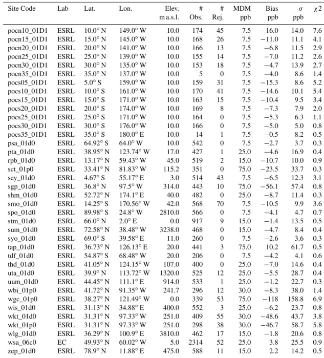
Table 2.Summary of the observation sites used in CarbonTracker-CH4, and the performance of the assimilation scheme at each site. “#Obs.” and “#Rej.” are the number of observations available and the number of observations for which the prior simulated concentrations deviate more than 3σ from the observations using a normal distribution defined with the observed value as the mean and the model–data mismatch error (MDM) as the standard deviation. The bias is the long-term mean of the posterior residuals (simulated-observed),σ is the standard deviation of the residuals for each site, and C2 is the chi-squared statistic calculated as the mean residual divided by the prior uncertainty (Simulated-Observed/(HQH+R); whereHis the matrix of transport response,Qis the prior flux uncertainty andR is the model–data mismatch error).
Site Code Lab Lat. Lon. Elev. # # MDM Bias σ χ2
m a.s.l. Obs. Rej. ppb ppb ppb
abp_01d0 ESRL 12.77◦S 38.17◦W 1.0 112 3 7.5 −8.4 7.7 2.0 alt_01d0 ESRL 82.45◦N 62.51◦W 200.0 532 0 15.0 −2.2 8.7 0.3 alt_06c0 EC 82.45◦N 62.51◦W 200.0 3181 10 15.0 −1.2 10.2 0.4 amt_01d0 ESRL 45.03◦N 68.68◦W 50.0 267 4 30.0 −6.1 22.8 0.4 amt_01p0 ESRL 45.03◦N 68.68◦W 50.0 174 0 30.0 0.8 16.5 0.3 asc_01d0 ESRL 7.97◦S 14.4◦W 74.5 961 79 7.5 −10.0 9.3 3.0 ask_01d0 ESRL 23.18◦N 5.42◦E 2728.0 491 0 25.0 −6.9 9.1 0.2 azr_01d0 ESRL 38.77◦N 27.38◦W 40.0 350 16 15.0 −12.0 15.9 1.7 bal_01d0 ESRL 55.35◦N 17.22◦E 3.0 974 0 75.0 1.4 29.4 0.1 bhd_01d0 ESRL 41.41◦S 174.87◦E 85.0 165 0 7.5 −4.1 5.4 0.7 bkt_01d0 ESRL 0.2◦S 100.32◦E 864.5 345 0 75.0 6.8 30.8 0.2 bme_01d0 ESRL 32.37◦N 64.65◦W 30.0 256 14 15.0 −13.6 17.4 2.1 bmw_01d0 ESRL 32.27◦N 64.88◦W 30.0 352 7 15.0 −13.2 12.8 1.4 brw_01d0 ESRL 71.32◦N 156.61◦W 11.0 514 13 15.0 −5.8 16.1 1.1 bsc_01d0 ESRL 44.17◦N 28.68◦E 3.0 501 1 75.0 −14.4 56.2 0.5 cba_01d0 ESRL 55.21◦N 162.72◦W 21.34 892 23 15.0 −10.6 13.4 1.1 cdl_06c0 EC 53.99◦N 105.12◦W 600.0 1390 77 25.0 −24.7 30.3 2.1 cgo_01d0 ESRL 40.68◦S 144.69◦E 94.0 416 0 7.5 −4.1 4.6 0.6 chr_01d0 ESRL 1.7◦N 157.17◦W 3.0 426 79 7.5 −14.6 9.9 5.2 crz_01d0 ESRL 46.45◦S 51.85◦E 120.0 453 0 7.5 −2.9 4.3 0.5 egb_06c0 EC 44.23◦N 79.78◦W 251.0 1810 0 75.0 −6.9 28.7 0.1 eic_01d0 ESRL 27.15◦S 109.45◦W 50.0 323 3 7.5 −7.3 5.3 1.4 esp_06c0 EC 49.58◦N 126.37◦W 7.0 403 0 25.0 −6.8 12.3 0.3 etl_06c0 EC 54.35◦N 104.98◦W 492.0 1780 135 25.0 −30.1 31.9 2.8 fsd_06c0 EC 49.88◦N 81.57◦W 210.0 3409 10 25.0 −9.4 18.3 0.6 gmi_01d0 ESRL 13.43◦N 144.78◦E 3.0 802 11 15.0 −10.2 13.0 1.2
hba_01d0 ESRL 75.58◦S 26.5◦W 30.0 506 0 7.5 0.5 4.6 0.3
Table 2.Continued.
Site Code Lab Lat. Lon. Elev. # # MDM Bias σ χ2
m a.s.l. Obs. Rej. ppb ppb ppb
pocn10_01D1 ESRL 10.0◦N 149.0◦W 10.0 174 45 7.5 −16.0 14.0 7.6 pocn15_01D1 ESRL 15.0◦N 145.0◦W 10.0 168 26 7.5 −11.0 11.1 4.1 pocn20_01D1 ESRL 20.0◦N 141.0◦W 10.0 166 13 7.5 −6.8 11.5 2.9 pocn25_01D1 ESRL 25.0◦N 139.0◦W 10.0 155 14 7.5 −7.0 11.2 2.6 pocn30_01D1 ESRL 30.0◦N 135.0◦W 10.0 153 18 7.5 −4.7 13.9 2.7 pocn35_01D1 ESRL 35.0◦N 137.0◦W 10.0 5 0 7.5 −4.0 8.6 1.4 pocs05_01D1 ESRL 5.0◦S 159.0◦W 10.0 159 31 7.5 −15.3 8.6 5.2 pocs10_01D1 ESRL 10.0◦S 161.0◦W 10.0 170 41 7.5 −14.6 10.1 5.4 pocs15_01D1 ESRL 15.0◦S 171.0◦W 10.0 163 15 7.5 −10.4 9.5 3.4 pocs20_01D1 ESRL 20.0◦S 174.0◦W 10.0 169 8 7.5 −7.3 7.9 2.0 pocs25_01D1 ESRL 25.0◦S 171.0◦W 10.0 164 0 7.5 −5.3 6.3 1.1 pocs30_01D1 ESRL 30.0◦S 176.0◦W 10.0 166 0 7.5 −5.0 5.0 0.8 pocs35_01D1 ESRL 35.0◦S 180.0◦E 10.0 14 1 7.5 −0.5 8.2 0.5
psa_01d0 ESRL 64.92◦S 64.0◦W 10.0 542 0 7.5 −2.7 3.7 0.3
pta_01d0 ESRL 38.95◦N 123.74◦W 17.0 427 1 25.0 −4.6 16.9 0.4 rpb_01d0 ESRL 13.17◦N 59.43◦W 45.0 519 2 15.0 −10.7 10.0 0.9 sct_01p0 ESRL 33.41◦N 81.83◦W 115.2 351 0 75.0 −23.5 33.7 0.3 sey_01d0 ESRL 4.67◦S 55.17◦E 3.0 514 43 7.5 −6.5 12.3 3.1 sgp_01d0 ESRL 36.8◦N 97.5◦W 314.0 443 10 75.0 −56.1 57.4 0.8 shm_01d0 ESRL 52.72◦N 174.1◦E 40.0 482 0 25.0 −8.7 11.4 0.3 smo_01d0 ESRL 14.25◦S 170.56◦W 42.0 568 70 7.5 −10.5 9.9 3.6 spo_01d0 ESRL 89.98◦S 24.8◦W 2810.0 566 0 7.5 −4.1 4.7 0.7
stm_01d0 ESRL 66.0◦N 2.0◦E 0.0 917 9 15.0 −1.4 13.5 0.5
sum_01d0 ESRL 72.58◦N 38.48◦W 3238.0 468 0 15.0 −4.7 8.4 0.4
syo_01d0 ESRL 69.0◦S 39.58◦E 11.0 260 0 7.5 −2.6 3.6 0.3
tap_01d0 ESRL 36.73◦N 126.13◦E 20.0 441 3 75.0 10.2 61.7 0.5 tdf_01d0 ESRL 54.87◦S 68.48◦W 20.0 206 0 7.5 −4.2 4.1 0.6 thd_01d0 ESRL 41.05◦N 124.15◦W 107.0 400 0 25.0 −7.0 14.6 0.4 uta_01d0 ESRL 39.9◦N 113.72◦W 1320.0 525 12 25.0 −5.5 28.7 0.4 uum_01d0 ESRL 44.45◦N 111.1◦E 914.0 533 1 25.0 −1.2 22.7 0.3 wbi_01p0 ESRL 41.72◦N 91.35◦W 241.7 296 12 30.0 −8.3 38.0 1.4 wgc_01p0 ESRL 38.27◦N 121.49◦W 0.0 339 53 75.0 −118 158.8 6.9 wis_01d0 ESRL 31.13◦N 34.88◦E 400.0 552 3 25.0 −6.2 23.7 0.8 wkt_01d0 ESRL 31.31◦N 97.33◦W 251.0 409 55 30.0 −48.6 43.7 3.8 wkt_01p0 ESRL 31.31◦N 97.33◦W 251.0 298 38 30.0 −46.7 58.7 5.8 wlg_01d0 ESRL 36.29◦N 100.9◦E 3810.0 462 17 15.0 −1.8 20.6 0.8
wsa_06c0 EC 49.93◦N 60.02◦W 5.0 2314 52 25.0 3.8 25.5 0.9
zep_01d0 ESRL 78.9◦N 11.88◦E 475.0 588 11 15.0 2.2 14.2 0.5
the Environment Canada sites also have large negative bi-ases. LLB (Lac Labiche, Canada) for example, has an aver-age residual of−80 ppb, and it is located close to possible wetland sources as well as fossil fuel operations.
3.2 Comparison to aircraft profiles
The current version of CarbonTracker-CH4does not
assim-ilate observations from the NOAA GMD aircraft project. This network currently consists of 17 sites distributed over North America where air samples are collected at 12 alti-tudes and analyzed for a suite of atmospheric gases, includ-ing CH4 (http://www.esrl.noaa.gov/gmd/ccgg/aircraft/).
Be-cause the aircraft observations were not used to constrain the
inversion, these data can be used as an independent check on the inversion. In addition, they provide useful insight into the performance of TM5’s vertical transport.
Figure 2.The CarbonTracker posterior residuals (simulated minus observed, in nmol mol−1) as a function of time and latitude (top) and prior residuals (bottom). Each dot represents the time and lo-cation of a CH4observation that was assimilated in CarbonTracker. Colors represent the difference between the final simulated value and the actual measurement, with warm colors indicating that Car-bonTracker simulates too much methane compared to observations, and cool colors indicating that CarbonTracker estimates too little.
location are more likely to sample background marine air coming off of the Pacific Ocean. In contrast, the continen-tal site, DND (Dahlen, North Dakota) shows a much larger negative bias at low altitudes during the summer but good agreement at all levels during winter (Fig. 5). This implies that local or regional-scale sources that are not included in the CarbonTracker-CH4 prior and are not “seen” by other
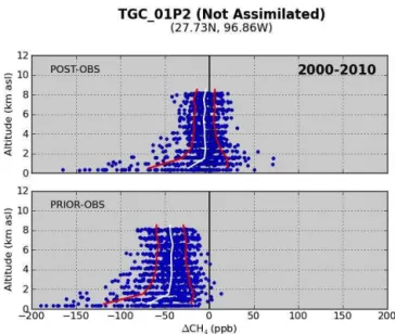
sites influence these summertime profiles. Similar results are found for other aircraft sites distributed throughout the cen-tral US Some sites, however, show larger biases near the sur-face. Figure 6 shows both prior and posterior residuals at TGC (Texas Gulf Coast), a site that sees both continental and marine air, and also air from nearby industrial and urban cen-ters along the Texas Gulf Coast. Even after the inversion, the residuals near the surface are still quite large indicating that the priors and the observations constraining are not able to account for strong local sources.
Figure 7 shows prior and posterior residuals for Poker Flat, Alaska. Note that even after the inversion, methane abun-dance is underestimated near the surface. This is likely the result of underestimation of prior wetland emissions, along with observational constraints that contain information about interior Alaska. On the other hand, as we will show be-low Arctic sites sampling background air likely capture the large scale methane budget fairly well. Figure 7 demon-strates the importance of sampling sites near sources for constraining regional methane budgets. Future versions of
Figure 3.The CarbonTracker posterior residuals (simulated minus observed, in nmol mol−1) as a function of time and latitude for North America. Each bubble has a radius proportional to the size of the residual, and the values are also indicated by the color bar. The largest residuals found by CarbonTracker-CH4are labeled also by site code.
Figure 5.Statistical summary of residuals for aircraft profiles at a site sampling continental air (Dahlen, ND; 47.5◦N, 99.2◦W). Units are 10−9mol mol−1of CH4(ppb). The top figure shows the post-assimilation residuals (posterior-observed) for winter months and the bottom figure shows the post-assimilation residuals for sum-mer months. Note that sumsum-mertime emissions near the surface are underestimated. Aircraft data are not currently assimilated in Car-bonTracker so they provide an independent evaluation of the data assimilation. Ideally, the mean of the residuals for the simulations with data assimilation should be near zero. The residuals for the simulations without data assimilation, on the other hand, tend to show large biases.
CarbonTracker-CH4may use at least the lower levels of the
aircraft observations in order to better constrain emissions.
3.3 Global and zonal averages
The abundance of CH4integrated over the global atmosphere
and its growth rate are important diagnostics of inversion per-formance (Rayner et al., 2005; Bruhwiler et al., 2011; Berga-maschi et al., 2013) because given the ∼10 yr lifetime of CH4, on global scales emissions and sinks must balance in a
way that produces the observed global growth of CH4. Here
we follow the approach taken by Bruhwiler et al. (2011) that uses the same sampling, filtering and smoothing procedure used to produce the observed global and zonal CH4
abun-dances for both data and model output (see Masarie and Tans (1995) and web updates at http://www.esrl.noaa.gov/gmd for a description of the data extension procedure). Zonal aver-ages are constructed using mainly marine boundary later sites by removing a long term trend approximated as a quadratic function, deseasonalizing by subtracting an average seasonal cycle, and using a low-pass digital filter with a half width of 40 days. Importantly, the model is sampled at the same times as the observations and missing data are filled in the same way for both the observations and simulations. The
simu-Figure 6.Statistical summary of residuals for aircraft profiles at a site sampling continental and marine air near strong local sources. Units are 10−9mol mol−1of CH4(ppb). The top figure shows the post-assimilation residuals (posterior-observed) for and the bottom figure shows the pre-assimilation residuals (prior-observed). The mean of the residuals for the simulations with data assimilation should be near zero. The residuals for the simulations without data assimilation, on the other hand, tend to show large biases.
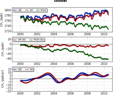
Figure 8.(Top) De-seasonalized time series of observed (dark blue, “OBS”, with very small error bars estimated using a bootstrap tech-nique), assimilated (red, “SIM”) and prior (green, “PRIOR”) av-erage methane mole fraction. For the “PRIOR” simulations, prior fluxes were used to calculate CH4 mole fractions, while for the “SIM” simulations CH4was calculated using fluxes that were ad-justed for optimal agreement with atmospheric observations. Units are ppb (10−9mol mol−1). (Middle) The differences from observa-tions for assimilated and prior CH4(ppb). (Bottom) Derived growth rate of CH4mole fraction for observed (with error bars) and assimi-lated CH4mole fraction. The growth rate is computed by taking the first derivative of the average mole fractions shown in the top figure. Units are ppb yr−1(10−9mol mol−1yr−1).
lated and observed zonal averages are therefore comparable. As shown in the top panel of Fig. 8, the global posterior CH4
abundance produced by the CarbonTracker-CH4assimilation
is in fairly good agreement with the observed global abun-dance, however it is biased low by about 10 ppb. This is be-cause the global abundance that results from use of the prior fluxes without optimization is much lower than observed, and the posterior global total represents a compromise be-tween CH4 abundance obtained from prior flux estimates
and the observations at each site. Reducing the model–data mismatch error and/or increasing the prior flux uncertainty would improve the agreement between posterior CH4 and
the observations, but likely at the expense of having flux es-timates with unrealistic spatiotemporal variability, especially in regions that are relatively unconstrained by observations. On the other hand, if the prior flux estimates are weighted too heavily in the inversion, the posterior global total more closely follows the global abundance simulated by the prior fluxes than the observations, and these may depart signifi-cantly from the actual emissions. The middle panel of Figure 8 shows the difference between the simulated and prior CH4
abundance and the observations, where it can be seen that the residual difference varies slightly over time as the bias
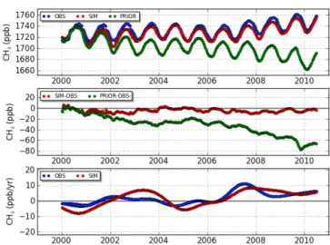
re-Figure 9.(Top) De-seasonalized time series of observed (dark blue, “OBS” with error bars), assimilated (red, “SIM”) and prior (green, “PRIOR”) average methane mole fraction for the polar Northern Hemisphere (53–90◦N). (Middle) Differences from observations for assimilated and prior CH4(ppb). (Bottom) Derived growth rate of CH4mole fraction for observed and assimilated CH4mole frac-tion for the polar Northern Hemisphere.
sulting from prior emissions changes. In particular, between 2004 and 2006, the prior residuals are fairly constant and the residual between the posterior and the observations is smaller than over other periods. The conclusions that can be drawn from this are that better prior flux estimates are needed for future versions of CarbonTracker-CH4, and that the global
abundance is a useful way to judge whether the solution is most influenced by the prior information or by the observa-tional constraints.
The bottom panel of Fig. 8 shows the growth rate of global atmospheric CH4, a quantity that is directly related to
im-balances between emissions and sinks. CarbonTracker-CH4
follows the observed growth rate fairly well, but not per-fectly since there are periods for which it under- or over-estimates the observed growth rate. During 2007, for ex-ample, the observed growth was underestimated by∼30 %, while during 2009 it was overestimated by about the same amount. These differences are an indication of global total biases in estimated emissions. The posterior global growth rate of CH4was also computed by Bergamaschi et al. (2013)
Figure 10.(Top) Time series of observed (dark blue, “OBS”), as-similated (red, “SIM”) and prior (green, “PRIOR”) average methane mole fraction for the tropics (17.5◦S–17.5◦N). (Middle) Differ-ences from observations for assimilated and prior CH4(ppb). (Bot-tom) Derived growth rate of CH4mole fraction for observed (with error bars) and assimilated CH4mole fraction for the tropics.
window, variability will be missed. As discussed by Bruh-wiler et al. (2005), an assimilation window of 12 weeks is ideal for the surface network, but computational issues pre-vented its use for this study. On the other hand Fig. 8 shows that the anomalous global growth is only slightly overesti-mated in 2003, while Bergamaschi et al. (2013) may under-estimate this feature.
It is also informative to consider zonally averaged CH4
mole fraction and its growth rate at sub-hemispheric scales as shown in Fig. 9 for the high northern latitudes (53.1–90◦N), Fig. 10 for the tropics (17.5◦S–17.5◦N) and Fig. 11 for the southern temperate latitudes (17.5–53◦S). For the high northern latitudes, the posterior simulated integrated CH4is
quite close to the observations and the growth rate agrees well with the observed growth rate. On the other hand, the simulated integrated CH4in the tropics is further from the
observations and closer to the prior than for the high north-ern latitudes. The posterior zonal average CH4abundance is
closer to the observations for the southern temperate latitude zone, however, the growth rate differences suggest some in-terannual variability differences, possibly the result of trans-port from tropical latitudes considering the relatively small contribution these latitudes make to the global methane bud-get. The simulated growth rate in the tropics also can dif-fer significantly from the observed growth rate, with under or over estimates reaching 5 ppb yr−1 or more. As a com-parison, the agreement between the observed and simulated growth rate at northern polar latitudes is usually well within a few ppb yr−1. The middle panels of Figs. 9, 10 and 11 show that when the residuals between the prior and observations decrease, the posterior residuals are also smaller.
Figure 11. (Top) Time series of observed (dark blue, “OBS”), assimilated (red, “SIM”) and prior (green, “PRIOR”) average methane mole fraction for the temperate Southern Hemisphere (17.5–53.3◦S). (Middle) Differences from observations for assim-ilated and prior CH4(ppb). (Bottom) Derived growth rate of CH4 mole fraction for observed (with error bars) and assimilated CH4 mole fraction for the tropics.
For the high northern latitudes, a small seasonal cycle in the residuals potentially provides some information about which emission processes may be under- or overestimated by the priors. Differences between simulated and observed CH4 are largest during the winter with the observations
be-ing higher than the simulations. This implies that mid- and high latitude emissions from anthropogenic sources may be underestimated by the priors and not completely corrected for by the inversion. Note that biogenic emissions at mid-and high latitudes are at a minimum during winter.
Anomalously high growth rates were observed in 2007 both in the Arctic and in the tropics (Dlugokencky et al., 2009), a year when the Arctic was anomalously warm and the tropics were unusually wet. The results shown in Fig. 9 sug-gest that the inversion is likely able to provide good estimates of flux anomalies in high latitudes, at least in the zonal av-erage. For the tropics, zonal average flux anomaly estimates for this year are likely to be underestimated. These differ-ences in the ability of the inversion to recover and attribute variability are due mostly to differences in the distribution of network sites with the Arctic having better observational cov-erage than the tropics. Another factor is that the deep vertical mixing of the tropical atmosphere makes it difficult for the network sites that are mostly located on remote islands to de-tect signals from terrestrial CH4sources. A further limitation
is the 5-week lag used in CarbonTracker’s EnKF (Ensemble Kalman Filter) scheme that cuts off transport of signals that are transported to remote observing sites.
prior covariance. If there are no observations to constrain the posterior estimates, then the posterior error covariance will be unchanged from the prior error covariance. While the pos-terior error covariance is a very useful diagnostic of the error reduction coming from observations, it is less useful as an indicator of the absolute accuracy of the estimated emissions because the accuracy of the prior estimates is ultimately not very well known, and there are transport errors that cannot be adequately accounted for.
4 Results
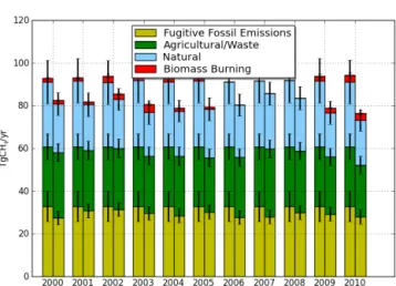
4.1 The high northern latitudes
Here the high northern latitudes are an aggregation of the Transcom 3 regions boreal North America, boreal Eurasia and Europe. This spatial division is somewhat awkward since some of Europe lies south of what could be considered high northern latitudes. We divide Europe into a northern section that lies poleward of 47◦N, and a southern section that is south of 47◦N, where this latitude is chosen to roughly cor-respond with the southern extents of boreal North Ameri-can and boreal Eurasian source regions. The prior anthro-pogenic emissions suggest that∼34 Tg CH4yr−1is emitted from northern Europe, while ∼15 Tg CH4yr−1 is emitted from southern Europe. Emissions from wetlands are much larger in the northern Europe than in the south.
The 10-year average posterior aggregated flux for the high northern latitudes is 81±7 Tg CH4yr−1, a decrease of a
lit-tle over 12 Tg CH4yr−1from the prior aggregated flux. Note
that due to the use of a 5-week assimilation window, the uncertainty estimate does not include temporal error covari-ance over timescales longer than this period and it should therefore be regarded as the best estimate possible for the long term error covariance given the limitations of the cur-rent assimilation scheme. The inversion suggests that most of this decrease is a reduction in natural wetland emissions (8 Tg CH4yr−1) with the remaining amount coming from
fugitive fossil fuel emissions, although the portioning be-tween these sources is strongly influenced by the prior distri-butions and relative locations of observation sites. Although the observing network could still be considered sparse at high northern latitudes, the number of existing sites is sufficient to reduce uncertainty by over 75 % from the prior uncertainty. The total posterior flux ranges from 78 Tg CH4yr−1in 2004
to just under 86 Tg CH4yr−1in 2007 (Fig. 12), a year that
saw record warm temperatures throughout much of boreal North America and boreal Eurasia, as well as extremely low sea ice coverage (Stroeve et al., 2008).
Annual average methane emissions at high northern lat-itudes are approximately evenly divided between fugitive emissions from fossil fuels, agriculture and waste (coming mostly from Europe) and natural wetlands. As a whole, emissions from fossil fuel leakage are slightly decreased
Figure 12.The contribution to the high northern latitude total CH4 flux from each category of emissions with 1-s error estimates. For each pair of histogram bars, the prior flux estimates are shown on the left and the posterior estimates on the right. Note that, except for emissions from fires, the prior flux estimates are constant for each year. The units are Tg CH4yr−1. The average estimated uncertainty on the total emissions is 7.5 Tg CH4yr−1.
relative to prior estimates by about 4 Tg CH4yr−1 from
33 Tg CH4yr−1, a change that is slightly larger than the
posterior estimated uncertainty, 3 Tg CH4yr−1. Note that
∼4 Tg CH4yr−1of the 29 Tg CH4yr−1due to fugitive
fos-sil fuel emissions comes from southern Europe. Emissions from agriculture and waste are unchanged. Annual average wetland emissions over the high northern latitudes are re-duced by 26 % from a prior of 31 Tg CH4yr−1 to about
23 Tg CH4yr−1, a difference that is larger than the average
estimated of ∼5 Tg CH4yr−1. This result is in agreement with previous studies (e.g., Chen and Prinn, 2006; Bergam-aschi et al., 2007; Spahni et al., 2011). Our results do not agree with the emission estimates of Bloom et al. (2010). They find that only 2 % of global wetland emissions come from the high northern latitudes, while we find closer to 10 %. On the other hand our results agree within uncertain-ties with the estimates of McGuire et al. (2012) based on flux measurements. They find a source of 25 Tg CH4yr−1 from
Arctic tundra wetlands with uncertainty ranging from 10.7 to 38.7 Tg CH4yr−1. Applying the same spatial filter for their
Arctic tundra region, CarbonTracker-CH4estimates a
The estimated flux anomaly during 2007 is 4.4±3.8 Tg CH4 with a maximum summer anomaly of
2.3 Tg CH4in July (Fig. 13). If the anomaly is calculated by
subtracting the 2000–2006 average annual flux the estimated 2007 anomaly is 5.3 Tg CH4, similar to the result found
by Bousquet et al. (2011). The results of Bergamaschi et al. (2013) also seem to be consistent with these estimates (1.2–3.2 Tg CH4). Based on zonal average analysis of
network observations, Dlugokencky et al. (2009) pointed out that in 2007 the global increase of methane was equal to about a 23 Tg CH4imbalance between emissions and sinks,
and that the largest increases in CH4growth occurred in the
Arctic (> 15 ppb yr−1). This does not necessarily imply that the largest surface flux anomalies occurred at high northern latitudes. Bousquet et al. (2011) noted that the relatively weak vertical mixing characteristic of polar latitudes results in a larger response in atmospheric CH4 mole fractions
to anomalous surface emissions than at tropical latitudes where strong vertical mixing rapidly lofts surface emissions through a deep atmospheric column. Transport models therefore can play an important role in helping to untangle surface flux signals from variability in atmospheric transport processes, although care must to be taken to also consider possible biases in modeled transport.
In 2008, the flux anomalies dropped to 2.4 Tg CH4, or
3 Tg CH4if the anomaly is calculated by subtracting the
av-erage annual flux over 2000–2006, as was done by Bous-quet et al. (2011) who obtained 2 TgCH4for their INV1 that
is similar to CarbonTracker-CH4, but−3 Tg CH4yr−1using
their higher spatial resolution variational inversion (INV2). As pointed out by Dlugokencky et al. (2009), both 2007 and 2008 were warm with higher than normal precipitation. Pos-terior covariance estimates support the independence of es-timates for boreal North America and boreal Eurasia since the covariance between these two regions is small; however, it is difficult to accurately relate variability in observed tem-perature and moisture anomalies with variability in estimated emissions because of the sparseness of the surface observa-tion sites.
For the high northern latitudes CarbonTracker-CH4is able
to distinguish between different CH4 source processes and
regions. Wetlands may be distinguished from anthropogenic sources because of the spatial separation of prior flux con-straints; many high northern latitude wetland complexes are located in relatively sparsely populated areas, while fossil fuel and agricultural and waste emissions are distributed mainly in populated areas of Europe (although the Western Siberian Lowlands is also a region of intensive fossil fuel production). Ocean methane fluxes are thought to be small compared to terrestrial fluxes, and northern Eurasia and bo-real North America are separated by the North Pacific Ocean. Furthermore, the stronger zonal and weaker vertical transport characteristic of the high latitudes helps to transport flux in-formation to network sites. Both Europe and boreal North America are at least partially constrained by surface network
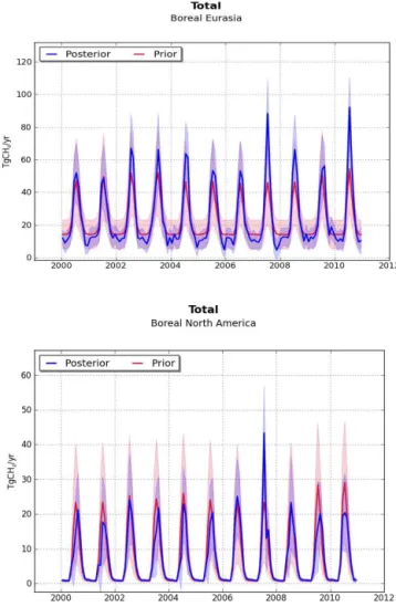
Figure 13.Time variation of the prior and estimated CH4 emis-sions. Prior estimates are shown in red, and posterior flux estimates are shown in blue. Note that only the biomass burning prior emis-sion estimates vary from year to year; other prior estimates are con-stant. 1σuncertainty bounds are shown as light red (prior) and light blue (post-assimilation) shaded areas. Note that microbial sources of methane, such as wetlands and agriculture, are temperature-sensitive and therefore tend to be largest during summer. Units are Tg CH4yr−1.
sites, and although boreal Eurasia is not adequately covered by network sites, a number of sites exist downwind of it (She-mya, Barrow and Cold Bay). For Europe, average trajectory calculations suggest that a large region of wetlands in eastern Scandinavia and northwestern Russia is constrained by Pal-las, Finland. Other sites help to constrain the anthropogenic sources from the rest of Europe.
from natural sources for Europe, the majority of which lie in northern Europe, are about 45 Tg CH4yr−1during the
sum-mer months while the 11 yr average posterior sumsum-mer es-timate is about 13 Tg CH4yr−1, a large reduction. The
un-certainty estimates, however, only decrease by at most 15 % implying that the source categories are not strongly con-strained by observations. Boreal Eurasian summertime wet-land emissions are increased relative to the prior flux esti-mates from 26 Tg CH4yr−1 to 37 Tg CH4yr−1, and
poste-rior uncertainties decrease from pposte-rior uncertainties by∼20– 25 %. For boreal North America, the average posterior sum-mer wetland flux is only slightly below the prior flux estimate (about 19 Tg CH4yr−1compared to about 16 Tg CH4yr−1,
a difference that is within the summer average posterior esti-mated uncertainty of∼10 Tg CH4yr−1). The redistribution
of emissions from Europe to northern Eurasia was found by Chen and Prinn (2006) to be sensitive to the choice of sites used in the inversion, however, our results indicate that the observations imply that while prior emissions are too high for Europe, larger emissions are still needed elsewhere to match the meridional distribution of observed methane. Bergam-aschi et al. (2005) also found decreased emissions for Eu-rope relative to prior estimates, but interestingly, their in-version also reduced high-latitude emissions from prior es-timates for other high latitude source regions as well. During the winter months, when biogenic emissions are low, prior estimates are decreased by the inversion for both boreal Eura-sia (−20 %) and Europe (−8 %) and relatively unchanged for boreal North America. The small change in winter European emissions supports the conclusion that prior wetland emis-sions for Europe are indeed overestimated. Note that prior emissions for wetland emissions from northern Europe are about equal to fugitive emissions from fossil fuels.
High latitude emissions of CH4from agriculture and waste
are significant only for Europe, and estimated fluxes are un-changed from prior estimates. Fugitive emissions of CH4
from fossil fuel production are reduced from prior estimates for Europe and boreal Eurasia by 2 Tg CH4yr−1for each
re-gion; from 21±4 Tg CH4yr−1and 12±2 Tg CH4yr−1. Re-ductions in uncertainty are fairly large for Europe,∼35 %, and about∼32 % for boreal Eurasia. For boreal North Amer-ica, prior estimates of fossil fuel emissions of CH4are very
small (< 1 Tg CH4yr−1), and it should be noted that the tar
sand production areas are in the temperate North American TransCom 3 source region rather than boreal North America. Significant natural CH4emissions have recently been
pro-posed for the high northern latitudes. Walter et al. (2007) estimated that in addition to emissions from high northern latitude wetlands (31 Tg CH4yr−1 for the
CarbonTracker-CH4 prior), ebullition from arctic lakes could add an
ad-ditional 24±10 Tg CH4yr−1. In addition to organic rich sediments and subsea permafrost, CH4 is stored in ice
hy-drates forming at the low temperatures and high pressures in sediments at the bottom of the Arctic Ocean and subsea permafrost, and below terrestrial permafrost as well.
Rela-tively shallow waters make it possible for bubbles to trans-port methane directly and rapidly to the atmosphere. The estimates of Shakhova et al. (2013) estimate the size of the source from subsea permafrost from the East Siberian shelf alone to be∼17 Tg CH4yr−1, although observational records are currently insufficient to establish whether these emissions are changing over time. Walter et al. (2012) have proposed that a similar process may also occur on land as permafrost thaws and glaciers melt. Total natu-ral emissions including all of these processes approaches 65 Tg CH4yr−1, an amount that significantly exceeds both
the average prior and posterior annual natural emissions for CarbonTracker-CH4(31 and 23 Tg CH4yr−1). Since the
av-erage total posterior CarbonTracker-CH4 high northern
lat-itude emissions is ∼81 Tg CH4yr−1, accommodation of a
65 Tg CH4yr−1 natural source would have to come at the
expense of fossil fuel and agriculture/waste sources (aver-age total CarbonTracker-CH4posterior of∼57 Tg CH4yr−1,
with about 12 Tg CH4yr−1 emitted from southern Europe),
which would need to be reduced by about 75 %.
The estimated mass of carbon thought to be frozen in Arc-tic permafrost down to 20 m is estimated to be∼1700 Pg C (Pg=1015g) (Tarnocai et al., 2009), significantly more car-bon than is currently in the atmosphere (∼830 Pg C) and over 3 times what has already been emitted to the atmosphere from fossil fuel use since pre-industrial times. As the Arctic warms and permafrost thaws, this ancient carbon may be mo-bilized to the atmosphere and a small fraction (∼3 %) may be emitted as CH4(Schuur et al., 2011). Recent studies suggest
that permafrost carbon will begin to enter the atmosphere during this century (e.g., Schaefer et al., 2010; Harden et al., 2012; Melton et al., 2013; Frolking et al., 2011). Harden et al. (2012) predict that 215–380 PgC will thaw by 2100. Their assessment of the carbon balance of Arctic tundra based on flux observations McGuire et al. (2012) found that between the 1990s and 2000s emissions of CH4 doubled (from 13
to 26 Tg CH4yr−1), results that are consistent with warmer
temperature and longer growing seasons.
Detection of trends in Arctic greenhouse gas emissions is difficult using atmospheric concentration measurements alone because changes are expected to be small in compari-son to transport of much larger mid-latitude emissions. For-ward and inverse modeling techniques can be helpful be-cause they provide the ability to untangle variability coming from transport from signals associated with local sources. As shown in Fig. 13, posterior CarbonTracker-CH4emissions do
not indicate that there has been a trend in natural high north-ern latitude emissions over the last decade, although we see strong evidence for substantial inter-annual variability.
4.2 The Northern Hemisphere mid-latitudes