Abstract
In this work, a vibration-based method for damage detection at welded beams and rods is presented. The model of the structural element includes the effect of the added inertia due to the welding process. Two methods of solution, analytically and by means of the Finite Element Method (FEM), are presented. From the results ob-tained it can be asseverated that the method can be a useful tool to detect degradation of welded structures. In contrast to other exist-ing methods for cracks detection, it is shown that several frequencies have to be taken into consideration to determine the wear charac-teristics of the welded elements, since depending on the location of welding, some frequencies can be very little sensitive to the reduc-tion of rigidity at the welded secreduc-tion. The results presented show similar tendency to those obtained by other investigations for cracks detection when added inertia was not included.
Keywords
Vibrations, welding, damage detection, non-destructive testing
Vibration-Based Method for Damage
Detection at Welded Beams and Rods
1 INTRODUCTION
Welded connections may have inelastic behavior due to failure, an incorrect welding procedure or the stresses supported on their working life (Gomaa et al., (2014); Shang et al., (2003)). To verify the wear of the welded element, non-destructive testing methods (NDT) have to be applied. Among others, some methods are: visual inspection, radio-logical methods, ultrasound scanning, thermo-graphic methods and acoustic emission (Halmshaw, (1987)). With most of them the structure has to be scanned on the precise site where the welding has been executed which sometimes might be inac-cessible. As examples, one can think of large structures like bridges, oil platforms, aircraft, ship struc-tures, etc.
Vibration-based methods (VBM) are a real alternative to classical NDT. In fact, VBM have certain advantages: the test equipment is relatively cheap, the vibration data can be collected from a
P. Salgado Sáncheza P. López Negroa P. García-Fogedab
aGraduate Student, ETSIAE, UPM,
Madrid, Spain
b Professor, ETSIAE, UPM, Madrid,
Spain
Author email:
http://dx.doi.org/10.1590/1679-78252881
simple point or mostly on several points on the structural component, and having an access to the damaged section is not required. Therefore, a method able to measure global parameters of structures that could provide information on the structural integrity from a few selected measurement points is very attractive for non-destructive testing (Smart and Chandler, (1995); Sohn et al., (2001)).
When a welding section fails, or starts to fail, on an elastic structural element, the damage intro-duces local flexibility due to strain energy concentration. This effect has been already recognized and the idea of an equivalent spring has been used to quantify, in a macroscopic way, the relation between the applied load and the strain concentration around the welded section like in Adams et al. (1978). This model has also been used for fatigue damaged structural elements, and to simulate the presence of cracks. Dimarogonas, (1996) presents a review on this problem. In the case of crack detection by VBM, different approaches have been developed. In some cases, lumped models for elastic massless elements have been used (Adams et al, (1978); Chondros and Dimarogonas, (1980); Rizos and Aspragathos, (1990); Morassi, (2000); Loya et al, (2006); Kindova-Petrova, (2014)), in others, a modified rigidity matrix has been employed in the Finite Element Method (Kisa, (2000); Saavedra et al. (1996)) and also a model of distribution of rigidity on the beam based on fracture mechanics methods has been used (Chondros et al. (1998 a)) and Chondros et al. (1998 b)); Chondros and Labeas, (2007)). In the problem of crack detection, not only the determination of the presence and size of the crack is important but also its location. Abdel-Mooty (2014) used a different approach to treat the identification of cracks based on the computation of the higher derivatives of structural modes for detecting the precise location of damage. Recently, the method has been applied for more complex systems like for crack detection on fluid-conveying pipes by Eslami et al (2016) and to solve the inverse problem of crack size and location based on the natural frequencies for an Euler-Bernoulli beam by Mostafa and Tawfik (2016). However, we are only interested in determining the quality or degradation of the welded section, showing that the added mass by the welding process has to be incorporated when modelling the system in order to reproduce the welded element behavior accu-rately.
The purpose of this paper is then to develop a robust and cost effective monitoring system for welded structural elements. The concept has also been applied to other welded systems like the work by Yunnus et al. (2011). After extreme events, such as earthquakes or blast loading, or due to aging and degradation resulting from operational environments, a welded section may reduce its structural properties and NDT based on vibration measurements can be a rapid condition screening to provide, in near real time, reliable information regarding the integrity of the structure. In this investigation, it is assumed that the structural element has a linear dynamic behavior before and after damage, and the detected damage is only due to the failure of the welded section. In addition, other problems due to environmental or operational conditions are assumed to not produce changes in the system re-sponse.
First, in section 2.1 the model is solved analytically for both structural elements. The nonlinear characteristic equation to determine the natural frequencies of the element can have, for some values of the parameters, a slow convergence. Thus, a FEM model has also been developed in section 2.2 based on the same scheme as the analytical method. The main advantage of the FEM is the ability to treat more complex boundary conditions than the analytical solution. Both methods are compared to determine the minimum number of elements of the FEM to assure convergence. From then on, only the results of the FEM are considered in section 3.
The results presented show that the method can be applied for damage detection of welded struc-tural elements. Attention shall be drawn to two particular points: the number of nastruc-tural frequencies used for the evaluation and the added inertia during the welding process. Conclusions are presented in section 4.
2 ANALYTICAL AND FINITE ELEMENT MODEL
As mentioned, two methods have been developed to determine the dynamic characteristics of a welded rod or beam. One is based on the analytical formulation, for the treatment of ideal boundary condi-tions, and the other on the Finite Element Method (FEM). The first one ends up with a highly nonlinear characteristic equation that is to be solved for any value of the different parameters involved in the model definition. This can be sometimes difficult, when regular nonlinear methods may converge very slowly. Therefore, it is used as a test method to determine the number of elements to be used in the FEM model to ensure convergence for a fix set of parameters and ideal boundary conditions.
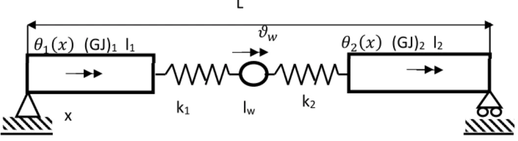
Figure 1: Model of the welding bond - torsion problem.
2.1Analytical Model
For linear analysis, torsion and bending dynamics can be considered decoupled. Then, two elementary structures are considered in this work: a uniform rod and a uniform Euler-Bernoulli beam. The total length of the element is L and it is assumed that, at the location l1, the element has been repaired by a welding connection.
In the case of a rod (see Figure 1), the welding is modeled as a lumped inertia element of value
w
I attached to the rod by two linear mass-less springs of rigidity k1 and k2. In this way, the failure or degradation of the soldering on either side of the welded section can be investigated. The differential equations and the boundary conditions for the system are then:
L
k
GJ l
GJ l
k
l
w2
1 1
1
2 0, 0 ;
GJ I x l
x x t
q q
-æ ¶ ö 
¶ ç ÷÷
-= £ £
ç ÷
ç ÷
ç
¶ è ¶ ø ¶ (1a)
2
2 2
1
2 0, ;
GJ I l x L
x x t
q q +
æ ¶ ö 
¶ ç ÷÷ - = £ £
ç ÷
ç ÷
ç
¶ è ¶ ø ¶ (1b)
(
)
1
1 w 1 at 1;
GJ k x l
x
q
J q
-
= - =
¶ (1c)
(
)
2
2 2 w at 1;
GJ k x l
x
q
q J +
= - =
¶ (1d)
(
)
(
)
¨
1 1 2 2 ;
w w w w
I J =k J -q -k q -J (1e)
where Jw is the generalized coordinate which determines the rotation of the lumped inertia term due
to the welded material, q1and q2 are the dynamic deformation of the rod at 0£ £x l1-and
1 ,
l+ £ £x L respectively, GJ the torsion rigidity of the rod, and I the polar moment of inertia per unit length of the rod.
Equations (1a) to (1e) should be completed with the ideal boundary conditions at the rod ends. For the case of simple supported end conditions (q1
( )
0 =0andq2( )
L =0), equations (1a) to (1e) can be solved to obtain the characteristic equation:(
)
(
)
(
)
(
)
(
)
(
)
2 2
1 2 2 1
2 1 2 1 2
cos sin sin cos sin sin
1 1 1 1
1 cos sin cos sin 0,
1 1 1
X X X X X X X X
s X X X X X X X
d d d d
l l l
l l l l
d d d d
l l l
l l l
æ ö é÷ ù æ ö é÷ ù
ç ÷ ê + ú +ç ÷ ê + ú +
ç ÷ ç ÷
ç ÷ ê ú ç ÷ ê ú
ç + + ç + +
è ø ë û è ø ë û
é + ù é ù é ù
ê ú ê ú ê ú
+ -ê + + ú ê + ú ê + ú =
+ + +
ë û ë û ë û
(2)
where the different parameters are:
2
1 2 2
1 1 2
1
, L 1, Iw, k L, k L and I.
X l s
l IL GJ GJ GJ
w
b l d d b
= = - = = = =
The roots of equation (2) can be obtained numerically for the unknown frequency parameter b
Figure 2: Non-ideal boundary conditions.
To guaranty the convergence of the FEM model for specific values of the parameters, the results for the first four natural frequencies have been calculated as function of the number of elements NFE
and compared with the results of the analytical solution. In this way, the analytical solution is used to validate the FEM model in both cases.
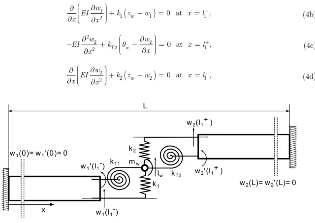
For the case of an Euler-Bernoulli beam in bending vibration, the model considered is illustrated in Figure 3. The mass added by the welding process is represented by a lumped mass of value mw and a rotational moment of inertia Iw. This mass is attached to both sides of the beam by two linear translational springs of value k1 and k2, and two linear rotational springs of values kT1 and kT2, all of them with zero inertia. The linear translational (torsion) springs oppose to vertical displacements (rotation) between both sides of the beam.
For the uniform beam considered, the formulation of the vibration problem can be expressed as:
2 2
2
1 1
1
2 2 2 0, 0 ;
w w
EI m x l
x x t
-æ ¶ ö 
¶ çç ÷÷÷+ = £ £
ç ÷
ç ÷
¶ è ¶ ø ¶ (3a)
2 2
2
2 2
1
2 2 2 0, ;
w w
EI m l x L
x x t
+
æ ¶ ö 
¶ çç ÷÷÷+ = £ £
ç ÷
ç ÷
¶ è ¶ ø ¶ (3b)
(
)
(
)
¨
1 1 2 2 0;
w w w w
m z +k z -w +k z -w = (3c)
¨
1 2
1 2 0;
w w T w T w
w w
I k k
x x
q + çççæq -¶ ÷ö÷÷÷+ æçççq -¶ ÷÷÷ö÷=
ç ¶ ç 
è ø è ø (3d)
and the conditions at x =l1 are given by Equations (4a) to (4d).
2
1 1
1 1
2 T w 0 at ,
w w
EI k x l
x
x q
-æ ö
¶ ç ¶ ÷
÷
- + çç - ÷÷= =
ç 
è ø
¶ (4a)
k
BC,Tk
BC,wθ
x
w x
(
)
1
1 1 1
2 w 0 at ,
w
EI k z w x l
x x
-æ ¶ ö
¶ ç ÷÷ + - = =
ç ÷
ç ÷
ç
¶ è ¶ ø (4b)
2
2 2
2 1
2 T w 0 at ,
w w
EI k x l
x
x q
+
æ ö
¶ ç ¶ ÷
÷
- + ççç - ÷÷= =
è ø
¶ (4c)
(
)
2
2 2 1
2 w 0 at ,
w
EI k z w x l
x x
+
æ ¶ ö
¶ ç ÷÷ +
- = =
ç ÷
ç ÷
ç
¶ è ¶ ø (4d)
Figure 3: Model of the welding bond - bending problem.
where zw and qw are the generalized coordinates which determine the translation and rotation of the
lumped inertia term due to the welded material, w1 and w2 are the dynamic deformation of the beam at 0£ £x l1-and at l1+ £ £x L, respectively; EI the flexural rigidity of the beam and m the mass per unit length of the beam.
These equations have to be completed with the boundary conditions at both ends of the beam. In the case of a clamped beam at both ends, the characteristic equation to determine the natural frequencies can be obtained by expansion of a determinant of order 6 (two of the constants of inte-gration can be eliminated from the boundary conditions) that depends on the following parameters:
3 3
1 2
1 2 3
1
1, mw, k L , k L , Iw , L
s r
l mL EI EI q mL
l = - = d = d = =
2
1 2 4
1 2
T , T and .
T T
k L k L
EI E
m E
I I
w
d = d = b =
Like in the previous case of the torsional rod, the resulting characteristic equation can be solved numerically to determine the natural frequencies of the system from the roots of the frequency pa-rameter. However, for this case the numerical solution is even more cumbersome than for the rod vibration element. Therefore again, the above formulation is only used as a measure of the convergence with the number of elements of the developed FEM model, based on the system of Figure 3. Again,
x w1(l1-)
w1'(l1-) w
2'(l1+ )
w2(l1+ )
kT2 kT1 k2 k1 mw Iw
w2(L)= w2'(L)= 0
w1(0)= w1'(0)= 0
the advantages of the FEM model are the ability to treat other type of end boundary conditions and to take any value of the different parameters defined before.
2.2 Finite element model for rod and the beam structural elements
Based on the classical formulation of the finite element method, see for example Petyt (1990), the dynamic problem is formulated as
{ }
¨
0,
M u K u
ì ü ï ï ï ï ï ï
é ùí ý+é ù = ë ûï ï ë û
ï ï ï ï
î þ (5)
where éëMùûand é ùë ûK corresponds to the mass and inertia matrix of the model, and
{ }
u is a vector containing the nodal displacements. This formulation is general for both cases -torsion and bending.Beginning with the torsion problem, the welded moment of inertia Iw, and the stiffness’s of the junctions between welding and the rod k1 and k2, are included in the formulation through the ele-ments in the mass matrix and stiffness matrix as
1 1
1 1 2 2
2 2
0 0 0 0
0 0 , .
0 0 0 0
w
w w
k k
M I K k k k k
k k
é ù é - ù
ê ú ê ú
ê ú ê ú
é ù =ê ú é ù = -ê + - ú
ë û ê ú ë û ê ú
-ê ú ê ú
ë û ë û
(6)
The same can be done for the bending problem, just taking into account that every node has then two degrees of freedom (vertical displacement and in-plane rotation). The resulting matrices for the bond are given by Equation (7).
1 1
1 1
1 2 2
1 2 2
2
2
0 0 0 0
0 0 0 0 0
0 0 0
, .
0 0
0 0 0
0
T T
w w
w T T T
T
k k
k k
M k k k
M K
I k k k
sym sym k
k
é ¼ ù é - ¼ ù
ê ú ê ú
ê ¼ ú ê - ú
ê ú ê ú
ê ¼ ú ê + - ú
ê ú ê ú
é ù =ê ú é ù = ê ú
ë û ê ¼ú ë û ê + - ú
ê ú ê ú
ê ú ê ú
ê ú ê ú
ê ú ê ú
ë û ë û
(7)
The stiffness and mass matrices of the whole model are built by the assembly of the local matrices of every single element: rods/beams for the structural element, and the previous matrices to represent the welding connection.
{
}
, ; beam / rod, welding connection
i i
i i
M M K K i
é ù = é ù é ù = é ù " Î
ë û
ë û ë û
ë û (8)( 1) 12
( 1) ( ) ( )
22 11 12
( ) 22
( 1) ( 1)
11 12
( 1) ( 2) ( 2)
22 11 12
0 0
0
0 ,
0
N
N N N
N
N N
N N N
M
M M M
sym M
M
M M
sym M M M
sym
-+ +
+ + +
éé ù ù
êê ú ú
êê ú ú
êê + ú ú
êê ú ú
êê ú ú
êêë úû ú
ê ú
é ù = ê ú
ë û ê ú
é ù
ê ê úú
ê ê úú
ê ê + úú
ê ê úú
ê ê úú
ê ê úú
ê ú
ë ë û û
w I (9a) ( 1) 12
( 1) ( ) ( )
22 11 12
( )
1
22 1
1 1 2 2
( 1) ( 1)
2 11 12
2
( 1) ( 2) ( 2)
22 11 12
0 0 0 0 , 0 N
N N N
N
N N
N N N
k
k k k
k
k k
K k k k k
k k k
k
sym k k k
-+ + + + + é ù ê ú ê ú + ê ú ê ú
ê + - ú
ê ú
ê ú
é ù = ê - + - ú
ë û ê ú
+
ê - ú
ê ú
ê + ú
ê ú ê ú ê ú ë û (9b)
where éëMùû( )11n is the component
{ }
1,1 of the mass matrix corresponding to the n-th element (and n = Nis the last element of the left side of the rod/beam). This procedure is also applied to the stiffness matrix. It can be observed that the resulting matrices are tridiagonal.Coming back to Equation (5), one can impose a harmonic movement in order to find the eigenmodes of the structure:
{ } { }
u = q ei tw,(10)
{
-w2[M]+[ ]K}
{ }
q ei tw =0.(11)
T his results in an eigenvalue problem for the natural frequencies like:
{
2}
{ }
2{ }
det -w ëéMûù+ë ûé ùK = 0 ë ûé ùK F = -w éëMùû F , (12) where wis the natural frequency and
{ }
F is the eigenvector.The number of elements has been determined by comparison of the FEM model to the analytical solution. It has been assured that the first four natural frequencies obtained by both means are close enough for a given set of parameters.
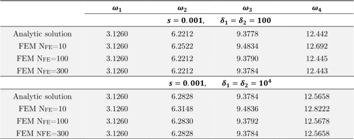
In Table 1 the evolution of the first six non-dimensional natural frequencies for a simple supported rod are calculated as a function of the number of elements for the values of the parameters l=1,
0.001
negligible. Therefore, it is concluded that -with this number of elements- the results of the FEM model are accurate enough.
. ,
Analytic solution 3.1260 6.2212 9.3778 12.442
FEM NFE=10 3.1260 6.2522 9.4834 12.692
FEM NFE=100 3.1260 6.2212 9.3790 12.445
FEM NFE=300 3.1260 6.2212 9.3784 12.443
. ,
Analytic solution 3.1260 6.2828 9.3784 12.5658
FEM NFE=10 3.1260 6.3148 9.4836 12.8222
FEM NFE=100 3.1260 6.2830 9.3792 12.5678
FEM NFE=300 3.1260 6.2828 9.3784 12.5658
Table 1: Convergence of the torsion problem FEM model given masses (s) and stiffness’s (d1 =d2) of the welded bond.
In Table 2 the first four non-dimensional natural frequencies for a beam clamped at both ends are presented as function of the number of elements. The values of the parameters are l=1,
0.001
s = , rq =0.0001 and different sets of the translational and torsional rigidities. The results of the characteristic equation are also given for comparison. Now, it can be observed that the number of elements to achieve a negligible difference has to be between 10 and 100. From now on, the number of elements used for the analysis of this structure will be . The rigidity at both sides of the lumped mass was kept for this validation case equal, i.e., d1 =d2 and dT1 =dT2.
Free beams: [ , ] Rigid bond: [ , ]
Analytic solution 0.0142 0.1414 14.349 14.349 22.373 61.671 119.68 199.83
FEM NFE=10 0.0142 0.1276 14.350 14.350 22.216 62.498 119.74 199.48
FEM NFE=100 0.0140 0.1415 14.350 14.350 22.212 62.497 119.73 199.44
FEM NFE=300 0.0091 0.0906 14.350 14.350 22.212 62.497 119.73 199.44
Damaged bond: [ , ] [ , . ]
Analytic solution 15.768 64.016 91.930 141.37 14.086 14.142 30.335 87.310
FEM NFE=10 15.774 61.693 91.935 137.52 14.087 14.127 30.338 87.315
FEM NFE=100 15.774 61.692 91.930 137.52 14.087 14.128 30.338 87.312
FEM NFE=300 15.774 61.690 91.929 137.52 14.087 14.127 30.338 87.312
Table 2: Convergence of the bending problem FEM model for a given mass (s = 0.01, rq = 0.0001) and various parameters of stiffness of the welded bond.
3 RESULTS AND DISCUSSION
Next, based on the FEM results, a study of the influence of the different parameters on the natural frequencies of the two problems considered -the welded rod and beam structural element- will be presented. The objective is to determine how a degraded welded joint can influence on the natural frequencies of the system. Thus, by means of a vibration test, be able to estimate the degradation of the element.
3.1 Rod Structural Element: Torsional Vibrations
The parameters considered for the torsion vibrating rod are the mass parameter , the position of the welded section l, the non-dimensional left-side spring rigidity d1, and the non-dimensional right-side spring rigidity d2, as defined in section 2.1. The initial values of all the parameters are such that the rod natural frequencies when welded are similar to those of the rod before damaged. Certainly, it could happen that the welded structural element has better dynamic properties (more rigidity) than the undamaged rod. This case, however, will not be considered in this paper.
The parameters can be estimated as follows:
( )
, ~ .
( )
s s s
s
IL L GJ IL L s
IL L d GJ IL L
~ ~ ~
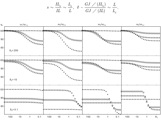
Figure 4: Evolution of the first four natural frequencies (percentage respect to the frequencies of the undamaged rod, wi u, ), for l=1 (solid), l =2 (circles) and l=3 (cross), with the variation of d1
and three fixed values of d2. A value of d2 =250, d2 =10 and d2 =0.001 represents, respectively, a rigid, a damaged and a broken bond.
60 80 100
60 80 100
100 10 1 0.1 60
80 100
100 10 1 0.1 100 10 1 0.1 100 10 1 ω1/ω1,u ω2/ω2,u ω3/ω3,u ω4/ω4,u
δ2= 250
δ2= 10
δ2= 0.1
%
In the first part of the study the mass parameter is kept to a constant value of s = 0.01 (the welding is performed using a material with a similar density to the rod and its length is about a 1% of the rod’s length), meaning that the amount of welded material remains the same with respect to the mass of the rod. The influence of the change of this parameter will be taken into consideration afterwards.
In Figure 4, the degradation of only one side of the welding -via reducing only one non-dimensional stiffness- is investigated, while keeping the other side stiffness constant. The plots show the evolution of the first four natural frequencies with the degradation of the left-side spring for different values of the stiffness of the right-side spring. Note that, as expected, the variation of the natural frequencies is bigger when both sides of the welding are affected.
From this figure the following conclusions can be obtained. For l=1, welded at the center of the rod, the odd frequencies are barely affected by the degradation. Thus, methods for crack detection based on the evolution of the first natural frequency may be unreliable for these cases. Higher order frequencies are more sensitive to rigidity losses than lower order, thus while the second frequency almost remains unchanged for l=1 and d2 =250 in the range of d1 between [250-50], the fourth frequency has a constant value in the reduced range of [250-100], concluding then that if the vibration method is used to determine the damage of a structural element several frequencies should be taken into consideration.
Forl=2, the odd frequencies are more affected by the rigidity variation. When the order of the frequency is increased the range of rigidity at which the frequency remains constant is also reduced. Thus, w1 w1,u ~ 1 for d1 Ì[250-50] and w4 w4,u for d1 Ì[250-100], although the change is less significant. For example, for d1 =1, w1/w1,u = 0.8 and w4 /w4,u =0.9. Then, it can be con-cluded that higher order frequencies are more sensitive to damage of the welded rod but lower order frequencies show biggest decrease when welding fails.
From the results shown in Figure 4, also the dynamic characteristics of the system as function of the different values of the parameters can be described. Thus, when the rigidity of the welded element is very small, the system behaves like two independent rod elements with a frequency close to the smaller frequency of a rod simply supported at one end and free at the other. This behavior is repre-sented -in a schematic way- as a function of the parameter l for the first modes in Figure 5.
The frequency parameter n, defined as n =w
( ) ( )
IL GJ , is used. For the undamaged rod it is named as ni u, and for the damaged rod ni js l,, . The first subscript means the mode order, the secondthe value of the parameter land the superscript refers to the shorter ‘’s’’ or larger ‘’l’’ uniform rod element for the damaged rod when l ¹1. When the rod is undamaged the frequency parameter has the values π, 2π, 3π… If the rod is welded at the middle point l =1and the section is broken, both parts of the rod have the same frequencies and the values are π, 3π, 5π… so the first two frequency parameters of the undamaged rod π and 2π collapse to a single frequency parameter of the broken rod π, the third and fourth frequency parameters collapse to the second frequency parameter of the broken rod 3π, and so on.
one, the frequency parameter s,2 i
n has the values 3π/2, 9π/2, 15π/2 for the first three frequencies and for the larger part l,2
i
n the values 3π/4, 9π/4, and 15π/4. Now, the undamaged frequencies move in the following way, n1,u moves from π to 3π/4, n2,u from 2π to 3π/2, and n3,4 from 3π to 9π/4, and
so on.
Similar reasoning can be made to explain the evolution of the natural frequencies for the other locations of the welding, for example l=3. In this way, it can be concluded that when one of the torsional rigidities is negligible and the other is such that the system prefers vibrating like two inde-pendent elements, the mode selected by the structure is the nearest one with smaller frequency of the cantilevered rod. Note that the relation between the frequencies of the undamaged rod and the broken one (cantilevered) matches with the plots given in Figure 4.
Figure 5: First non-dimensional frequencies of the rod in different conditions: with no damage on the
welding ni u, and without being welded ni j, . First subindex ‘’i’’ denotes the i-th mode of vibration
(i.e., 1, 2, 3...), the second denotes the values of the parameter l, and the letter ‘’s’’ or ‘’l’’ if the side under consideration is the shorter or the larger one when l ¹1, respectively. Finally, the different
curved arrows are related to the value of l considered: 1 (thick) and 2 (thin).
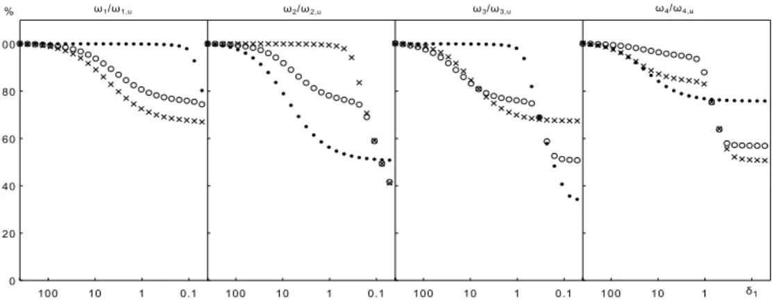
Figure 6: Evolution of the first four natural frequencies (percentage respect to the frequencies of the undamaged rod,wi u, ), for l =1(solid), l =2(circles) and l =3(cross), with the variation of d1
(both springs have the same rigidity, d1 =d2).
π 2π 3π 4π
3π/4 3π/2 9π/4 15π/4
υ1,u υ2,u υ3,u υ4,u
υ1, 2l υ1, 2s υ2, 2l υ3, 2s
υ1, 1 υ2, 2l υ2,1
0
s δ1
δ2
100 10 1 0.1 0
20 40 60 80 100
100 10 1 0.1 100 10 1 0.1 100 10 1 δ1
Now, in Figure 6 the general damage of the welding is considered. For d1 =d2, both sides of the welding with equal rigidity, the first four natural frequencies divided by the natural frequency of the undamaged rod are presented as function of the parameter d1 for l=1, 2, 3 (welded section at 50%, 33% and 25% of the total length, respectively). In the figure it can be observed that the analysis of several frequencies has to be used to detect the damage of the welded section. When the welding is close to a node, there is a large concentration of stresses at the point and therefore the dynamic response is more sensitive to small changes in rigidity. This can be observed in the second and fourth frequencies forl=1, and in the third frequency forl=3. When damage on the welding is investi-gated, one is interested in detecting this damage as early as possible and, as Figure 6 suggests, the higher order of the frequency the more sensitive to decrease on rigidity. However, on real structures higher order frequencies can also be influenced by other parameters i.e., aging of the structure. There-fore, a careful analysis of all the frequencies should be made to asseverate the quality of the welding.
In addition, note that there is a critical value of d1 and d2 where the system prefers to respond as a single vibrating lumped mass when the smaller frequency of the cantilevered rod coincides with
(
d1 +d2)
s, written in non-dimensional parameters.In this way, one can see that starting with high values of d1 and d2 the behavior of the model will be similar as the clamped-clamped rod (undamaged). Decreasing the stiffness of the rod will lead to a change of the natural frequencies, which will tend to the corresponding frequencies of the clamped-free (cantilever) rods, as shown in Figure 5. Moreover, when the smaller frequency of the cantilever rods (corresponding to the longer structural element) is greater than
(
d1 +d2)
s lower frequencies will be found, but these frequencies will be associated to the motion of the lumped mass. This behavior can be observed in Figure 6 when both sides are really damaged. These values of didemonstrate the model's consistency.
This result is very interesting, as it opens a further study: while at least one of the two sides of the bonds remains undamaged the lumped mass will vibrate attached to one of the structural element. If a frequency close to that of the cantilever rod is found, then one can asseverate that at least one of the two sides of the welding is highly damaged and the bond is very close to failure.
For damage detection the most important parameter is the change in frequency, independently to the damage occurring at one or both sides of the welding connection. When welding fails the natural frequencies of the system are those of the cantilever rod (slightly modified by the influence of the attached lumped mass). Therefore, no further results will be presented varying independently the two sides of the welding connection.
0.0125
s = , the rigidities should be modified up to a value of 725. So, a 25% increase from the value 0.01
s = in the welding mass leads to a 382% increase in both rigidities. Even more, there is a critical mass value when no rigidity is enough to recover the natural frequency of the undamaged rod.
s
2
0.0010 53 55 196 48
0.0050 78 81 196 72
0.0100 190 192 196 180
0.0125 725 600 196 690
0.0150 - - 196 -
3
0.0010 103 0.023 107 193
0.0050 130 0.23 134 193
0.0100 196 18 193 193
0.0125 265 - 246 193
0.0150 400 - 340 193
Table 3: Value of the nondimensional rigiditiy d1 to recover the i-th frequency of the first four
natural modes with the variation of the nondimensional welding mass . It was takend1 =d2.
Some interesting cases can be observed in the table. Forl=2, in the mass interval of interest, no stiffness changes are needed to keep constant the frequency of the third mode. This effect can be explained in terms of the eigenmodes. The third mode presents a node where the welding is placed, so there is no displacement during the vibrations in this section and therefore, the mass does not affect. The same reasoning could be applied to the fourth frequency withl=3. In addition, the effect of the strains/stresses concentration could be considered (via the derivative of the rotation). For
3
3.2 Beam Structural Element: Bending Vibrations
Next, the dynamic characteristics of an Euler-Bernoulli beam element are investigated as function of the different parameters.
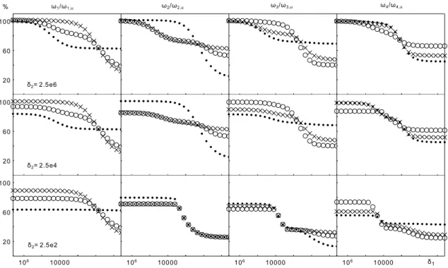
Figure 7: Evolution of the first four natural frequencies (percentage respect to the frequencies of the
undamaged beam,wi u, ), for l=1(solid), l=2(circles) and l=3(cross), with the variation
of d1 and three fixed values of d2. A value ofd2 =250, d2 =10 and d2 =0.001 represents, respectively, a rigid, a damaged and a broken bond.
Now, the parameters to modify are the nondimensional inertia properties and rq, the position of the welded section l, the nondimensional translational rigidities d1 and d2, and the nondimensional torsional rigidities dT1 and dT2 of the left and right-side springs, respectively. Note that, each side of
the welding is affected by both translational and torsional rigidities and it has no physical sense to consider the isolated effect of one of them. Therefore, the study will be focused on damage either the right or the left-side on the welding bond via decreasing both rigidities.
In this way, we estimate s r, , q d and dT to be
3
2 3
3 2 3
( )
~ s ~ s, ~ s ~ s , ~ s ~ and ~ s ~ ,
T
s s
mL L mL L L EI L L EI L L
s r
mL L q mL L d EI L L d EI L L
æ ö÷
ç ÷
ç ÷
ç ÷
çè ø
20 60 100
20 60 100
106 10000
20 60 100
106 10000 106 10000 106 10000 δ1
% ω1/ω1,u ω2/ω2,u ω3/ω3,u ω4/ω4,u
δ2= 2.5e6
δ2= 2.5e4
where Ls is the welding length, and the beam slenderness. Again, a welding material similar to the structural one is considered. From this analysis we could also infer the ratio between nondimensional translational and torsional stiffness’s of each side given by ddT ~ 10000. From now on, the rela-tionship di dTi =10000 will be always used. Like for the rod in torsional vibration, we consider a welding length of a 1% of the total length and =10 to be consistent with the applicability of the Euler-Bernuilli beam theory.
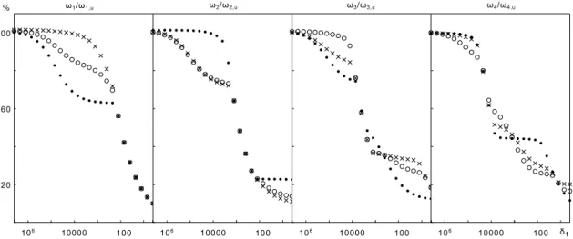
The mass parameters s = 0.01 and rq =0.0001 will be kept constant like in the prior study. The effect of damaging one side of the welding section will be considered first. In Figure 7 the first four natural frequencies are given for different values of the right-side stiffness’s with the variation of the left-side rigidities.
In this figure it can be observed the following: for the case of l=1, in contrast with the case of torsional vibration, now all the frequencies, odd and even, are reduced when decreasing rigidity and the reduction can be quite large (closer to 80% for the second frequency when rigidity is low). These results were also observed for a similar model but without lumped mass by Loya et al (2006) and Priyadarshini (2013). Also, for the same frequencies (see w3 w3,u) there are two transitions as
function of the rigidity, one when the rigidity decrease to a value of 104 and a second one when the reduction is closer to a value of 102. The evolution of the frequency in this case can serve as a measure of the grade of the structure.
Now for the bending vibration case, it seems that the influence of the location of welding, values of l=1, 2, 3 in Figure 7, seems to be not as important as in the torsion case since now, for all the
locations and frequencies, there is a reduction in frequency when rigidity is decreased.
From this figure, similar conclusions to the rod structural element could be drawn. Defining a new nondimensional frequency parameter n = w (mL3)
( )
EI , the first four natural frequencies ofa double-clamped undamaged beam ui u, (where the subscript ‘’i’’ denotes the i-th mode) are given
by 22.37, 61.67, 120.90 and 199.86. In addition, following a similar nomenclature we call ( ) ,
s l i j
n to the
i-th frequency of the shorter (larger) cantilevered beam for a value of l =j. When the beam is undamaged the frequency parameter coincides with the double-clamped beam natural frequencies in each mode.
Moreover, one can estimate the threshold where the lumped mass vibrations appears. The trans-lational and rotational frequencies for the lumped mass -written in a dimensionless nomenclature- are given by
(
d1 +d2)
s and(
dT1 +dT2)
rq, respectively. The ratio could by written as1 2
' 1 2
~ ~ ~
w
w T T T s
r r L
s s L
q q
u d d d
u d d d
+
+
that, for the welding length considered, is 10. Therefore, for a really damaged -practically broken- soldering, the system will vibrate first as a translating lumped mass.
Figure 8: Evolution of the first four natural frequencies (percentage respect to the frequencies of the undamaged beam,wi u, ), for l=1(solid), l =2(circles) and l=3(cross), with the variation of d1
(both springs have the same rigidity,d1 =d2, dT1 =dT2 and dT1 =10-4d1).
Now, in Figure 8 the evolution of the first four frequencies of the damaged beam referred to the value of the frequency of the undamaged beam are represented as function of the nondimensional rigidityd1. For this figure it was set d1 =d2 anddT1 =dT2. Three positions of the welding are consid-ered defined by the values of the parameterl=1, 2 and 3.
From the figure it is observed that the first frequency is the one that changes more rapidly for 1
l= and the second frequency for l =2, 3. With a reduction of rigidity from 106 to 105 the fre-quency already changes to a value of 80% for the first frefre-quency (referred to the frefre-quency of the undamaged structure) andl=1; and a similar reduction is observed for the second frequency when
2, 3
l = . Thus, the method can serve as a good prediction method of damage detection when the reduction of stiffness is still very low.
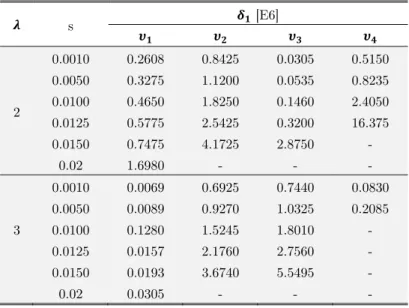
Finally, the effect of welding inertia is considered. The results are presented in Table 4 and it can be observed again that when the added mass is large (a 2% of the total beam mass) it is no longer possible to recover the dynamic properties of the undamaged beam for all cases (in fact it is only possible for the first frequency, withl =2). The amount of added mass that limit the go back to the
106 10000
20 60 100
106 10000 106 10000 106 10000
100 100 100 100 δ1
ω1/ω1,u ω2/ω2,u ω3/ω3,u ω4/ω4,u
undamaged beam depends on the welded position, thus, for l=3the fourth frequency cannot be recovered for a value of added mass of 1%. This is a very interesting result for the evaluation of damage of welded structural elements since depending on the added mass, somehow it is needed the starting state of the welded structural element before it can be evaluated if the bond is damaged or not.
s [E6]
2
0.0010 0.2608 0.8425 0.0305 0.5150
0.0050 0.3275 1.1200 0.0535 0.8235
0.0100 0.4650 1.8250 0.1460 2.4050
0.0125 0.5775 2.5425 0.3200 16.375
0.0150 0.7475 4.1725 2.8750 -
0.02 1.6980 - - -
3
0.0010 0.0069 0.6925 0.7440 0.0830
0.0050 0.0089 0.9270 1.0325 0.2085
0.0100 0.1280 1.5245 1.8010 -
0.0125 0.0157 2.1760 2.7560 -
0.0150 0.0193 3.6740 5.5495 -
0.02 0.0305 - - -
Table 4: Value of the nondimensional rigidities d1 to recover the i-th frequency of the first
four natural modes with the variation of the nondimensional welding mass andrq. We take rq =s 100 andd1 =d2 =10000dT1 =10000dT2.
4 CONCLUSIONS
A method for the evaluation of the dynamic properties of welded structural elements has been pre-sented. The method can consider any real boundary condition of the element and applications to simpler boundary conditions have been presented.
For the simplest boundary conditions, the analytical approach can be used, leading to a non-linear equation. However, even in these cases, the convergence of numerical methods is arduous. On the other hand, the FEM model can treat different boundary conditions and the eigenvalue method is accurate and fast.
The impact of the welding characteristics in the system response has been presented and dis-cussed. The main conclusion that can be inferred is that soon when rigidity at either side of the welding is decreased the dynamic characteristics of the structural element change enough to be de-tected. Section 3 presents the most part of the results, where one can see the evolution of the first natural frequencies for different values of the welding stiffness. In fact, this change of the natural frequencies allows to determine the damage of the welding bond. It might be interesting to quantify this damage experimentally to fully validate the proposed method in this work.
structural element cannot be recovered. This is a very interesting result since if the method of vibra-tion test is used to detect the damage of a welded element, a reducvibra-tion of the natural frequencies could already exist from the moment when the element was repaired, due to the added mass. Thus, the dynamic properties of the welded element should be the base to compare with and not the dynamic properties of the undamaged structural element.
Another conclusion that can be drawn from the results presented is that, in general, several frequencies should be considered when evaluating if a welded structural element is damaged. Depend-ing on the weldDepend-ing location the first frequency may not be affected by the loss of rigidity at the bond connection. This result is in contrast to other investigations that used a vibration based method to determine the damage of a beam due to cracks and considered only the change of the first natural frequency.
References
Abdel-Mooty, M. (2012). Damage Identification in Continuous Structures Using Free Vibration Characteristics. 10th World Congress on Computational Mechanics, July 2012, Sao Paulo, Brazil.
Adams, R.D., Cawley, P., Pye, C.J. and Stone, B.J. (1978). A vibration technique for non-destructively assessing the integrity of structures. Journal of Mechanical Engineering Science. 20:93-100.
Chondoros, T.G. and Labeas, G.N. (2007). Torsional Vibration of a Cracked Rod by Variational Formulation and Numerical Analysis. Journal of Sound and Vibration 301:994-1006.
Chondros, T.G. and Dimarogonas, A.D. (1980). Identification of cracks in welded joints of complex structures. Journal of Sound and Vibration. 69:531-538.
Chondros, T.G., Dimarogonas, A.D. and Yao, J. (1998 a)). A Continuous Cracked Beam Vibration Theory. Journal of Sound and Vibration. 215:17-34.
Chondros, T.G., Dimarogonas, A.D. and Yao, J. (1998 b)). Longitudinal Vibration of a Continuous Cracked Bar. Engineering Fracture Mechanics. 61:593-606
Dimarogonas, A.D. (1996). Vibration of Cracked Structures: A State of the Art Review. Engineering Fracture Me-chanics. 55:831-857.
Eslami, G., Maleki, V.A. and Rezaee, M. (2016). Effect of Open Crack on Vibration Behavior of a Fluid-Conveying Pipe Embedded in a Visco-Elastic Medium. Latin American Journal of Solids and Structures. 13 (1):136-154.
Gomaa, F.R., Nasser, A.A. and Ahmed, Sh.O. (2014). Sensitivity of Modal Parameters to Detect Damage through Theoretical and Experimental Correlation. International Journal of Current Engineering and Technology. 4:172-181. Halmshaw, R. (1987). Nondestructive Testing. Edward Arnold.
Kindova-Petrova, D. (2014). Vibration-Based Methods for Detecting a Crack in a Simply Supported Beam. Journal of Theoretical and Applied Mechanics, 44:69-82.
Kisa, M. and Brandon, J. (2000). The Effects of Closure of Cracks on the Dynamics of a Cracked Cantilever Beam. Journal of Sound and Vibration. 238:1-18.
Loya, J.A., Rubio, L. and Fernandez-Saez, J., (2006). Natural frequencies for bending vibrations of Timoshenko cracked beams. Journal of Sound and Vibration 290:640-653.
Morassi, A. (2001). Identification of a Crack in a Rod Based on Changes in a Pair of Natural Frequencies. Journal of Sound and Vibration. 242:577-596.
Mostafa, M. and Tawfik, M. (2016) Crack Detection Using Mixed Axial and Bending Natural Frequencies in Metallic Euler-Bernuilli Beam. Latin American Journal of Solids and Structures. 13(9):1641-1657.
Priyadarshini, A. (2013). Identification of Cracks in Beams Using Vibration Analysis. Master Science Thesis. Depart-ment of Civil Engineering. National Institute of Technology, Rourkela, India.
Rizos, P.F. and Aspragathos, N. (1990). Identification of Crack Location and Magnitude in a Cantilever Beam from the Vibration Modes. Journal of Sound and Vibration. 138:381-388.
Saavedra, P., Baquedano, D. and San Juan, L. (1996). Modelo Numérico para el Estudio Dinámico de un Rotor con Eje Agrietado. Revista Internacional de Métodos Numéricos para Cálculo y Diseño en Ingeniería. 12:125-146.
Shang, D., Barkey, M.E., Wang, Y. and Lim, T.C., (2003). Effect of Fatigue Damage on the Dynamic Response Frequency of Spot-Welded Joints. International Journal of Fatigue. 25:311-316
Smart, M. and Chandler, H.D. (1995). Modal testing for NDT of structures. R and D Journal. 11:79-85.
Sohn, H., Farrar, C.H., Fugate, M.L. and Czarnecki, J.J. (2001). Structural Health Monitoring of Welded Connections. The First International Conference on Steel and Composite Structures, Pusan, Korea, June 14-16.