8(2011) 393 – 411
Estimation of RC slab-column joints effective strength using
neural networks
Abstract
The nominal strength of slab-column joints made of high-strength concrete (HSC) columns and normal high-strength con-crete (NSC) slabs is of great importance in structural design and construction of concrete buildings. This topic has been intensively studied during the last decades. Different types of column-slab joints have been investigated experimentally providing a basis for developing design provisions. However, available data does not cover all classes of concretes, rein-forcements, and possible loading cases for the proper calcu-lation of joint stresses necessary for design purposes. New numerical methods based on modern software seem to be effective and may allow reliable prediction of column-slab joint strength. The current research is focused on analysis of available experimental data on different slab-to-column joints with the aim of predicting the nominal strength of slab-column joint. Neural networks technique is proposed herein using MATLAB routines developed to analyze available ex-perimental data. The obtained results allow prediction of the effective strength of column-slab joints with accuracy and good correlation coefficients when compared to regres-sion based models. The proposed method enables the user to predict the effective design of column-slab joints without the need for conservative safety coefficients generally promoted and used by most construction codes.
Keywords
column-slab joint, effective strength, high strength column, normal strength slab, neural network, regression.
A. A. Shaha,∗ and Y. Ribakovb aSpecialty Units for Safety and Preservation of
Structures, College of Engineering, King Saud University, P.O. Box 800, Riyadh 11421 – Saudi Arabia
bDepartment of Civil Engineering, Ariel
Uni-versity Center of Samaria, Ariel – Israel
Received 05 Mar 2011; In revised form 31 May 2011
∗Author email: [email protected]
1 INTRODUCTION
The use of flat-plate system in tall buildings is rapidly increasing due to its advantages on structural performance and construction process over conventional RC (reinforced concrete) construction [10]. As a result this system has been adopted and widely used for many structures that were recently constructed such as large-scale supermarket, store and underground garage, bridge decks, etc. Using RC flat plate system in the basement and residential floors of tall
394 A.A. Shah et al / Estimation of RC Slab-column joints effective strength using neural networks
buildings is often mandatory to reduce story height and to enable rapid construction. The use of flat plate floors for the basement parking areas also minimizes the amount of excavation so that total construction time and cost can effectively be reduced [19].
Flat plate slab [6] is a very common and competitive structural system, in which columns directly support floor slabs without beams. Such system of construction usually consists of high strength concrete (HSC) columns and normal strength concrete (NSC) slabs or floors. The slabs are laid with NSC mainly for the purpose of achieving the economy and improving the ductile behavior. However, in some cases the presence of intervening weaker concrete slab layer affects the column load carrying capacity. The column strength is reduced as compared to its actual axial compressive strength [22].
Flat-plate systems are popular gravity systems permitting architectural flexibility, more clear space, simple formwork, shorter construction time and simple arrangement of electrical and mechanical systems. Buildings with such systems are technology-friendly and conducive to modern design concepts. Compared to a typical beam-slab system, the flat-plate slab-column system should be able to save structural costs by about 20%. Absence of efficient load transfer mechanism has been one of flat-plate system’s weak point that may lead to a brittle punching shear failure at the region of slab-column joint [7, 24]. It was found that the effective moment of inertia concept, together with the Direct Design Method, can be used for computing deflections of irregular flat plate floors [24]. Additionally, the results obtained indicated that at higher load levels, beyond the serviceability limit state, the use of reduced modulus of elasticity will improve the predicted deflections considerably [24]. The problem of brittle punching failure due to the transfer of shearing forces and unbalanced moments at the flat plate-column connection was investigated to study the effects of various interdependent factors that govern the punching shear resistance and behavior of the flat plate-column connections as well as their inclusion in current Codes [7]. It was shown that the problem of displacement-induced unbalanced moment and the accompanying shear forces at flat plate-column connections can be effectively addressed by providing shear reinforcement in slabs.
To understand the load transfer mechanism and predict the effective strength of the joint when two different strengths of concrete are used in columns and slab, several experimental investigations have been conducted [2, 8, 9, 15, 17, 20, 21]. The test results, obtained for slab-column specimens, were analyzed to determine the maximum difference between column and floor concrete strengths that yield no decrease in the column load-carrying capacity and the allowable load-carrying capacity of the column if this difference is exceeded [2].
The modern ACI code [1] provisions for estimating the strength of a slab-column joint are based upon the outcomes of this research [2]. It was also shown that the ACI code is unsafe for higher ratios of column to slab concrete strengths [8]. A separate design equation, as a function of column and slab concrete strengths, was proposed that tend to negate the ACI equation for estimating the joint effective strength [8].
Interior column specimens were also tested with and without load acting on a slab [17]. The slab loading on the tested specimens was of service nature and it was applied together with the ultimate axial load that acted on the column portions. It was shown that the slab
A.A. Shah et al / Estimation of RC Slab-column joints effective strength using neural networks 395
loading develop significant tensile strains in the slab’s top steel in the slab-column joint region. They recommended that the effective strength of the joint should not only be a function of column and slab concrete strengths but also of the joint aspect ratio (ratio of slab thickness to column dimension, h/c).
One interior slab-column joint was tested with extreme load acting on the slab and service axial load applied on the column [9]. It was reported that the joint strength is highly influenced by the bending action of the slab. It was found that the surrounding slab confinement increased the strength and ductility of the joint [15]. It was also reported that the use of fiber-reinforced concrete in slabs at interior columns increases the strength and stiffness of the joints.
A double headed shear stud rails was used in the surrounding slabs in order to improve the punching shear resistance of the test specimens [20, 21]. The slabs were loaded with ultimate load and columns with service axial load. The effects of surrounding slab confinement, ratio of slab thickness to column dimension (aspect ratio,h/c), intensity of slab load, slab reinforcement ratio, column concrete strength and slab concrete strength were investigated. It was found that the application of slab load reduces the column axial load carrying capacity. It was also observed that the ACI code [1] provisions are unsafe and non-conservative for test specimens with high aspect (h/c) and column to slab concrete strength ratios. The Canadian standard [5] was found safe but conservative for test specimens with low aspect (h/c) ratios. A new design expression, incorporating all of the above-mentioned parameters that is able to predict the joint effective strength more reliably than the ACI code [1] and Canadian standards [5] was proposed. Schematic views of different types of the tested slab-column joints are shown in Fig. 1.
Figure 1 Schematic views of slab-columns connection: (a) interior column (b) edge column (c) corner column (d) sandwich column (following [13]).
In this research the data of previous experimental researchers [2, 8, 9, 15, 17, 20, 21], involving the testing of slab-column connections with HSC columns and NSC slabs has been used. Analysis of the accumulated test data employing the neural network technique has been performed in order to develop a new procedure for predicting the effective strength of the slab-column joint. A neural network has the capability of realizing a greater variety of nonlinear relationship of considerable complexity [3, 23]. In neural networking the data is presented to the network in the form of input and output parameters, and the optimum nonlinear relationship is found by minimizing a penalized likelihood.
In fact, the network tests many kinds of relationship in its search for an optimum fit.
396 A.A. Shah et al / Estimation of RC Slab-column joints effective strength using neural networks
As in regression analysis, the results then consist of a specification of the function, which in combination with a series of coefficients (called weights), relates the inputs to the outputs. The search for the optimum representation can be computer intensive, but once the process is completed (that is, the network has been trained), the estimation of outputs is very rapid. This work has been applied to the complex problem of predicting the capacity of an interior slab-column connection.
The present study, applying neural networking, is also aimed at focusing efforts on bringing simplicity and improving the reliability of the proposed estimation procedure. Additionally, the use of test data covering a large range of column and slab concrete strengths, column and slab reinforcement ratios, surrounding slab confinement, and wide range of slab thickness to column dimension ratio (aspect ratio, h/c) greatly enhances the scope of the present study.
2 AIMS AND SCOPE OF THE RESEARCH
Despite the availability of large number of models, the problem of column-slab joint effective strength has remained inconclusive. It is felt that this is partly due to the complexity of the phenomenon involved and partly because of the limitations of statistical regression, an analytical tool commonly used by most of the investigators. Neural networks (NN) have advantages over statistical models like their data-driven nature, model-free form of predictions, and tolerance to data errors [11, 12, 16, 18]. The objective of this study is to reanalyze the data considered in earlier studies by employing the NN technique with a view towards finding out if better predictions are possible.
The current research is focused on analysis of available experimental data on different column-slab joints with the aim of predicting the effective column-slab joint strength. For this reason the NN technique was employed. Original MATLAB routines [13] were developed to analyze the available experimental data. NN toolbox is used to analyze the experimental data [14] and predict the effective column-slab joints strength. The prediction should have high accuracy and high correlation coefficients, compared to the regression based models in order to enable using the predicted results in effective design of column-slab joints with no need to conservative safety coefficients presently used in the codes.
3 EXISTING MODELS FOR ESTIMATING THE COLUMN-SLAB JOINT EFFECTIVE STRENGTH
A large number of regression models, mostly empirical, based on mechanics of structures and materials are available for the prediction of the effective strength of a column-slab joint [1, 2, 5, 8, 17, 20, 22]. ACI code [1] suggests that there is no reduction in column strength for ratios of column concrete strength to slab concrete strength up to 1.4. For higher ratios, based on the experiments by Bianchini et al. [2], the following expression for predicting the effective strength of the joint was proposed:
fcef f′ =0.75fcc′ +0.35fcs′ ; (1)
A.A. Shah et al / Estimation of RC Slab-column joints effective strength using neural networks 397
where,fcc′ and fcs′ are strength of column and slab concrete respectively.
Gamble and Klinar [8] proposed the following as a lower bound relationship for estimating the strength of a column-slab joint:
fcef f′ =0.47fcc′ +0.67fcs′ ; (2)
They reported that the ACI code [1] equation is adequate for column concrete strength to slab concrete strength ratio of 1.4. However, for higher ratios ACI code [1] design provision overestimates the effective strength of the joints and is therefore unsafe.
In existing design provisions to cover the high strength concrete, for higher ratios of col-umn concrete strength to slab concrete strength, the Canadian Standard CSA-A23.3:1994 [5] presents the following design expression:
fcef f′ =0.25fcc′ +1.05fcs′ ; (3)
The effective strength prediction using CSA A23.3 [5] design provisions appears to be safe but highly conservative.
A striking feature of the test programs conducted by both Bianchini et al. [2] and Gamble and Klinar [8] was the absence of slab load. In fact in a prototype structure, load on the slab will produce significant tensile straining in the top flexural slab reinforcement in the vicinity of the column. It would seem reasonable to assume that such strain will have a detrimental effect on the ability of the surrounding slab to confine the column-slab joint [17]. Ospina and Alexander [17] developed a new design model incorporating the effect of the ratio of slab thickness to column dimension (aspect ratio, h/c). The design equation, proposed for predicting the effective strength of the joint, is given as under:
fcef f′ = (0.25 h/c)f
′
cc+(1.4− 0.35
h/c)f
′
cs; (4)
Besides the column and slab concrete strengths as well as the aspect ratio (h/c), the effects of surrounding slab confinement and slab reinforcement ratio,rs, should also be considered in predicting the effective strength of the joint [20]. Based on the induction of the new parameters, the following predicting equation was devised:
fcef f′ =0.35fcc′ +0.384( ρs+4.12
h/c+1.47)λf ′
cs; (5)
Recently a mechanics of materials approach, commonly used for composite materials, was applied for the theoretical analysis of the problem [22]. This approach with the use of the available test data lead to a new regression model for calculating the effective strength of the joint. Additionally, it was reported that the new experiments [8, 9, 15, 17, 20, 21] tend to negate the limiting ratio of 1.4 between the two concrete strengths, which ACI [1] allows in Sec. 10.15 of its building code to be used without considering any adverse affects on the axial load carrying capacity of the columns. The effective strength of the joint concrete was found
398 A.A. Shah et al / Estimation of RC Slab-column joints effective strength using neural networks
to be proportional to the ratio of product and sum of the two concrete strengths, as given below:
fcef f′ =2.25( f ′ ccfcs′
f′ cc+fcs′
); (6)
This observation leads to the comparison of column specimens’ behavior with that of com-posite materials. The accumulated test data provides a strong evidence for the applicability of some mechanics principles of composite materials to the sandwiched concrete. Additionally, it is observed that most of the models presented above were developed by different researchers mainly for their own data, except the model proposed by Shah et al. [20], which has used a wide variety of data.
4 AVAILABLE EXPERIMENTAL DATA
Table 1 shows the test data of column-slab specimens with HSC columns and NSC slabs [2, 8, 9, 15, 17, 20] with total of 74 data points. The data consists of eight parameters viz. slab thickness, column dimension, column reinforcement, slab reinforcement, slab confinement factor, slab load, concrete strength of slab and column. The range of these parameters for the data is given in Table 2. The data covers all the possible four cases of confinement viz. interior column, edge column, corner column and sandwich column.
All the columns are square in size except two, as mentioned in Table 1, for which equivalent square section has been considered. The experimental value of effective strength of joint, given in the table, has been calculated from:
fcef f′ = Pc−fyAst
0.85(Ag−Ast)
(7)
where Pc is the maximum load carried by the column, Ast is the area of longitudinal steel bars in the column, Ag is the gross cross-sectional area of the column section, fy is the yield strength of column reinforcement, and fcef f′ is the effective concrete compressive strength. The effective strength, fcef f′ , is notionally the cylinder strength of some hypothetical concrete that combines the properties of both the column and slab concretes and can be expected to be in between the range of column and slab concrete strengths.
5 NEURAL NETWORK MODEL
The manner, in which the data are presented for training, is the most important aspect of the NN method. Often this can be done in more than one way, the best configuration being determined by trial-and-error. It can also be beneficial to examine the input and output patterns or data sets that the network finds difficult to learn. This enables a comparison of the performance of the NN model for these different combinations of data.
In order to map the causal relationship related to the slab-column joint strength, two separate input/output schemes (called Model-A1 and Model-A2) were employed. The first took
A .A . S h a h et a l / E st im a tio n o f R C S la b -c o lu m n jo in ts eff ec tiv e st re n g th u sin g n eu ra l n et w o rk s 399
Table 1 Details of column-slab specimens.
Source Specimen h c ρc ρs λa Pc Ps ps fy′ fcc′ fcs′ fcef f′
(mm) (mm) (%) (%) (kN) (kN) (kN/m2) (MPa) (MPa) (MPa) (MPa)
Bianchini et al. [2]
S9013.0 178 279 1.46 0.55 4 3114 0 0 310 51.0 17.1 42.1
S7513.0 178 279 1.46 0.55 4 3287 0 0 310 51.3 22.2 45.2
S75I3.0 178 279 1.46 0.55 4 2891 0 0 310 43.2 15.9 38.8
S60I3.0 178 279 1.46 0.55 4 3069 0 0 310 45.3 14.3 41.7
S60I2.0 178 279 1.46 0.55 4 3114 0 0 310 45.7 23.7 42.3
S50I2.0 178 279 1.46 0.55 4 2580 0 0 310 40.6 21.3 34.1
S50I2.0 178 279 1.46 0.55 4 2446 0 0 310 34.4 15.2 32.1
S40I2.0 178 279 1.46 0.55 4 1922 0 0 310 25.9 17.0 24.1
S45I1.5 178 279 1.46 0.55 4 2669 0 0 310 34.3 19.8 35.5
S37I1.5 178 279 1.46 0.55 4 2002 0 0 310 22.6 15.2 25.4
S30I1.5 178 279 1.46 0.55 4 1979 0 0 310 25.6 13.4 25.1
Gamble and Klinar [8]
C 178 254 1.76 0.71 4 3781 0 0 490 89.0 29.7 59.6
D 178 254 1.76 0.71 4 4670 0 0 490 96.5 30.3 76.5
G 178 254 1.76 0.71 4 4893 0 0 490 90.3 42.8 80.6
H 178 254 1.76 0.71 4 3336 0 0 490 85.5 17.2 51.7
K 178 254 1.76 0.97 4 5315 0 0 490 72.4 35.2 88.5
L 178 254 1.76 0.71 4 5115 0 0 490 83.4 33.1 84.7
Ospina and Alexander [17]
A1-A 100 200 3.53 0.58 4 3194 0 0 445 105 40 100.31
A1-B 100 200 3.53 0.65 4 3678 48 25 445 105 40 93.08
A1-C 100 200 3.53 0.65 4 3498 94 49 445 105 40 87.56
A2-A 100 200 3.53 0.43 4 3820 0 0 445 112 46 97.43
A2-B 100 200 3.53 0.65 4 3807 33.2 17 445 112 46 97.03
A2-C 100 200 3.53 0.65 4 3591 86 45 445 112 46 90.41
A3-A 150 200 3.53 0.35 4 3437 0 0 445 89 25 85.69
A3-B 150 200 3.53 0.85 4 3174 100 53 445 89 25 77.63
A3-C 150 200 3.53 0.85 4 2275 157.2 83 445 89 25 50.09
A4-A 150 200 3.53 0.35 4 3272 0 0 445 106 23 80.64
A4-B 150 200 3.53 0.85 4 2927 93.2 49 445 106 23 70.07
A4-C 150 200 3.53 0.85 4 2376 135.2 71 445 106 23 53.19
B-1 250 250 1.13 0.38 4 4072 173.2 95 445 104 42 71.54
B-2 250 250 1.13 0.75 4 5359 130 71 445 104 42 96.08
B-3 250 250 1.13 0.59 4 5078 173.2 95 445 113 44 90.72
B-4 250 250 1.13 0.44 4 6298 0 0 445 113 44 113.99
B-5 250 250 1.13 0.38 4 2703 172.2 94 445 95 15 45.44
B-6 250 250 1.13 0.75 4 3720 130 71 445 95 15 64.83
B-7b 250 175 1.15 0.59 4 2758 173.2 95 445 120 19 47.45
B-8b 150 175 1.15 0.75 4 4032 130 71 445 120 19 72.25
Jungwirth [9] J-1 150 200 4.62 1.45 4 3342 639 998 550 80 33 71.7
(Continued on next page)
400 A .A . S h a h et a l / E st im a ti o n o f R C S la b -c o lu m n jo in ts eff ec ti ve st re n g th u si n g n eu ra l n et w o rk s
Table 1 (continued)
Source Specimen h c ρc ρs λa Pc Ps ps fy′ fcc′ fcs′ fcef f′
(mm) (mm) (%) (%) (kN) (kN) (kN/m2) (MPa) (MPa) (MPa) (MPa)
Mcharg et al. [15]
NU 150 225 1.40 1.41 4 3008 0 0 486 81.8 30.0 62.8
NB 150 225 1.40 1.41 4 3254 0 0 486 81.8 30.0 68.6
Shah et al. [20]
ICSA-1ICSA-2 120 200 2.00 0.53 4 2858 348 544 545 85 32.0 73.0
120 200 2.00 1.00 4 3180 442 691 545 83 30.0 82.0
ICSA-3 120 200 2.00 0.53 4 2729 300 469 545 70 28.0 69.0
ICSA-4 120 200 2.00 1.00 4 3191 459 717 545 84 29.0 83.0
ICSC-1 180 200 2.00 0.36 4 2821 624 975 545 82 28.0 71.0
ICSD-1 240 200 2.00 0.43 4 2713 871 1361 545 79 32.0 68.0
Bianchini et al. [2]
S90E3.0 178 279 1.46 0.55 3 2526 0 0 310 52.5 16.8 33.4
S75E3.0 178 279 1.46 0.55 3 2375 0 0 310 46.9 16.4 30.9
S60E3.0 178 279 1.46 0.55 3 1966 0 0 310 35.8 11.9 24.6
S60E2.0 178 279 1.46 0.55 3 2589 0 0 310 45.1 23.9 34.3
S50E2.0 178 279 1.46 0.55 3 2015 0 0 310 35.3 16.2 25.4
S40E2.0 178 279 1.46 0.55 3 1615 0 0 310 23.2 9.6 19.4
S45E1.5 178 279 1.46 0.55 3 1984 0 0 310 23.8 17.7 25.2
S37E1.5 178 279 1.46 0.55 3 1779 0 0 310 20.8 13.7 22.0
S30E1.5 178 279 1.46 0.55 3 1543 0 0 310 15.8 10.1 18.3
Gamble and Klinar [8]
A 178 254 1.76 0.89 3 3336 0 0 486 86.2 28.3 51.7
B 178 254 1.76 0.89 3 3225 0 0 486 86.9 25.5 49.6
E 178 254 1.76 0.89 3 4226 0 0 486 90.3 45.5 68.2
F 178 254 1.76 0.89 3 3002 0 0 486 97.9 15.9 45.5
I 127 254 1.76 0.94 3 2891 0 0 486 92.4 30.3 68.2
J 178 254 1.76 0.89 3 4448 0 0 486 79.3 36.5 72.3
Bianchini et al. [2]
S90C3.0 178 279 1.46 0.54 2 2135 0 0 310 52.0 17.0 27.4
S75C3.0 178 279 1.46 0.54 2 2295 0 0 310 51.2 18.6 29.9
S60C3.0 178 279 1.46 0.54 2 1712 0 0 310 37.1 8.8 20.8
S60C2.0 178 279 1.46 0.54 2 2446 0 0 310 45.7 24.8 32.2
S50C2.0 178 279 1.46 0.54 2 2002 0 0 310 38.2 17.6 25.3
S40C2.0 178 279 1.46 0.54 2 1632 0 0 310 24.2 10.4 19.6
S45C1.5 178 279 1.46 0.54 2 1957 0 0 310 27.5 18.8 24.8
S37C1.5 178 279 1.46 0.54 2 1779 0 0 310 22.6 15.9 21.9
S30C1.5 178 279 1.46 0.54 2 1334 0 0 310 16.5 10.6 15.2
Bianchini et al. [2]
S75S3.0 178 279 1.46 0 0 1846 0 0 310 36.8 15.0 22.4
S60S2.4 178 279 1.46 0 0 1672 0 0 310 35.5 13.5 20.1
S50C2.0 178 279 1.46 0 0 1850 0 0 310 35.9 15.0 23.1
S37C1.5 178 279 1.46 0 0 1735 0 0 310 20.8 13.5 21.1
a Slab confinement factor,? = 4 for interior column, = 3 for edge column, = 2 for corner column, = 0 for sandwich column bRectangular column of 175
×250mm (Equivalent square considered) [1]
A.A. Shah et al / Estimation of RC Slab-column joints effective strength using neural networks 401
Table 2 Range of parameters for the data of slab-column connections (74 data points).
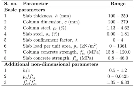
S. no. Parameter Range
Basic parameters
1 Slab thickness, h (mm) 100 – 250
2 Column dimension,c (mm) 200 – 279
3 Column steel,ρc (%) 1.13 – 4.62
4 Slab steel, ρs (%) 0.00 – 1.81
5 Slab confinement factor, λ 0 – 4
6 Slab load per unit area, ps (kN/m2) 0 – 1361 7 Column concrete strength, fcc′ (MPa) 15.8 – 120.0 8 Slab concrete strength, fcs′ (MPa) 8.8 – 46.0
Additional non-dimensional parameters
1 h/c 0.5 – 1.2
2 ps/fcs′ 0 – 0.0425
3 fcc′ /fcs′ 1.35 – 6.33
the input of raw causal parameters while the second utilized their non-dimensional groupings. This was done in order to check if the use of the grouped variables produced better results. The Model-A1 thus takes the input in the form of causative factors namely,h,c,ρc,ρs,λ,ps,
fcc′ and fcs′ yields the output, the joint-effective strength, fcef f′ :
Model-A1: fcef f′ =f(h, c, ρc, ρs, λ, ps, fcc′ , fcs′ ); (8)
The matrix of dimensions for the variables involved is:
A=⎡⎢⎢⎢
⎢⎢ ⎣
1 0 0 1 1 1 0 0 0
−1 1 1 −1 −1 −1 0 0 0
−2 0 0 −2 −2 −2 0 0 0
⎤⎥ ⎥⎥ ⎥⎥ ⎦
;
The columns of the above matrix correspond to the variables in the order in which they appear in Eq. (8) and the rows of the matrix correspond to the three fundamental dimensions viz. M (mass), L (Length) and T (Time). Though the number of fundamental dimensions involved in the model is three but the rank of the above dimensional matrix is 2, thus accord-ing to the Buckaccord-ingham-PI theorem [4], the number of dimensionless parameters required for modeling would be 9−2=7. The independent PI terms obtained from the nullity theorem are:
h/c, ρc,ρs,λ, ps/fcs′ , andfcc′ /fcs′ and the corresponding dimensionless outputfcef f′ /fcc′ . The Model A-2 employing these dimensionless variables is thus given by:
Model-A2: f ′ cef f
f′ cc =
g(h
c, ρc, ρs, λ, ps
f′ cs
,f
′ cc
f′ cs)
; (9)
The current study used the data described above (74 data points) for the prediction of joint effective strength. The training of the above two models was done using 67% of the data
402 A.A. Shah et al / Estimation of RC Slab-column joints effective strength using neural networks
(49 data points) selected randomly. Validation and testing of the proposed models was made with the help of the remaining 33% of observations (25 data points), which were not involved in the derivation of the model.
Three neuron models namely, ‘tansig’, ‘logsig’ and ‘purelin’, have been used in the ar-chitecture of the network with the back propagation algorithm implemented in originally de-veloped MATLAB routines. In the back propagation algorithm, the feed-forward (FFBP), cascade-forward (CFBP) and Elman back propagation (EBP) type network were considered [3, 11, 12, 16, 18, 23]. Each input is weighted with an appropriate weight and the sum of the weighted inputs and the bias forms the input to the transfer function. A transfer function (also known as the network function) is a mathematical representation, in terms of spatial or temporal frequency, of the relation between the input and output of a (linear time-invariant) system. With optical imaging devices, for example, it is the Fourier transform of the point spread function (hence a function of spatial frequency) i.e. the intensity distribution caused by a point object in the field of view.
The transfer function is commonly used in analysis of single-input single-output (SISO) filters. It is mainly used in signal processing, communication theory, and control theory. The term is often used exclusively to refer to linear time-invariant systems (LTI). Most real systems have non-linear input/output characteristics, but when operated within nominal (not “over-driven”) parameters they behave close enough to linear LTI systems. The neurons employed use the following differentiable transfer function to generate their output:
yj =f⋅(∑ i
Wijxi+φj) =
1
1+e−(∑iWijxi+φj); (10)
Linear transfer function:
yj =f⋅(∑ i
Wijxi+φj) =∑ i
Wijxi+φj; (11)
Tan-sigmoid transfer function:
yj =f⋅(∑ i
Wijxi+φj) =
2
1+e−2(∑iWijxi+φj) −1; (12)
The weight, w, and biases, f, of these equations are determined to minimize the energy function. The optimal architecture was determined by varying the number of hidden neurons. The optimal configuration was based upon minimizing the difference between the neural net-work predicted value and the desired output. In general, as the number of neurons in the layer is increased, the prediction capability of the network increases in beginning and then becomes stationary.
The performance of all NN model configurations was based on the mean percent error (MPE), mean absolute deviation (MAD), root mean square error (RMSE), correlation coef-ficient (CC), and coefcoef-ficient of determination, R2, of the linear regression line between the predicted values from the neural network model and the desired outputs. Training of NN
A.A. Shah et al / Estimation of RC Slab-column joints effective strength using neural networks 403
models was stopped when either the acceptable level of error was achieved or when the num-ber of iterations exceeded a prescribed maximum. The neural network model configuration that minimized the MAE and RMSE and optimized the R2 was selected as the optimum and the whole analysis was repeated several times.
6 SENSITIVITY ANALYSIS
Sensitivity tests were conducted to determine the relative significance of each of the indepen-dent parameters (input neurons) on the joint effective strength (output) in both of the models given by Eqs. (8) and (9). In the sensitivity analysis, each input neuron was in turn eliminated from the model and its influence on prediction of effective strength of the joint was evaluated in terms of the MPE, MAD, RMSE, CC and R2 criteria. The effect of elimination of two and more independent variables on the effective strength of joint has also been studied. The network architecture of the problem considered in the present sensitivity analysis consists of one hidden layer with 12 neurons and the value of epochs has been taken as 100.
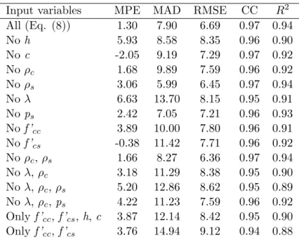
Table 3 Sensitivity analysis of Model A-1 with feed-forward back propagation for different sets of input vari-ables.
Input variables MPE MAD RMSE CC R2
All (Eq. (8)) 1.30 7.90 6.69 0.97 0.94
Noh 5.93 8.58 8.35 0.96 0.90
Noc -2.05 9.19 7.29 0.97 0.92
Noρc 1.68 9.89 7.59 0.96 0.92
Noρs 3.06 5.99 6.45 0.97 0.94
Noλ 6.63 13.70 8.15 0.95 0.91
Nops 2.42 7.05 7.21 0.96 0.93
Nof ’cc 3.89 10.00 7.80 0.96 0.91
Nof ’cs -0.38 11.42 7.71 0.96 0.92
Noρc,ρs 1.66 8.27 6.36 0.97 0.94
Noλ,ρc 3.18 11.29 8.38 0.95 0.90
Noλ,ρc,ρs 5.20 12.86 8.62 0.95 0.89
Noλ,ρc,ps 4.22 11.23 7.59 0.96 0.92
Only f ’cc,f ’cs,h,c 3.87 12.14 8.42 0.95 0.90
Only f ’cc,f ’cs 3.76 14.94 9.12 0.94 0.88
Note: MPE, mean percent error; MAD, mean absolute deviation; RMSE, root mean square error;
CC, correlation coefficient;R2, coefficient of determination.
The results in Table 3 show that for Model-A1, slab thickness, h, slab confinement factor,
λ, column concrete strength,fcc′ , slab concrete strength,fcc′ , and column steel,ρc, are the five most significant parameters for the prediction of effective strength of the joint. The variables in the order of decreasing level of sensitivity for Model-A1 are: h, λ, fcc′ , fcs′ , ρc, c, ps and
ρs. It is thus seen that the last three parameters have least significant effect when taken independently. The influence of the removal of two and more independent parameters at a
404 A.A. Shah et al / Estimation of RC Slab-column joints effective strength using neural networks
time has also been studied for some of the pairs. Some of the pairs considered for removal represent the existing models. The sensitivity analysis by eliminating all except fcc′ and fcs′
represents models given by Eqs. (1) to (3) and (6). It is observed to have significant effect as it reduces the value ofR2 from 0.94 to 0.88. Thus the models of Bianchini et al. [2], Gamble and Klinar [8], Canadian Standards [5] and Shah and Ribakov [22] have ignored some useful parameters. The elimination of all except fcc′ ,fcs′ , h and c representing the model given by Eq. (4), is also observed to have significant effect as it reduces the value of R2 from 0.94 to 0.90. The model given by Eq. (5) is simulated by eliminating λ,ρc and ps in Table 3, which reduces the value ofR2 from 0.94 to 0.92.
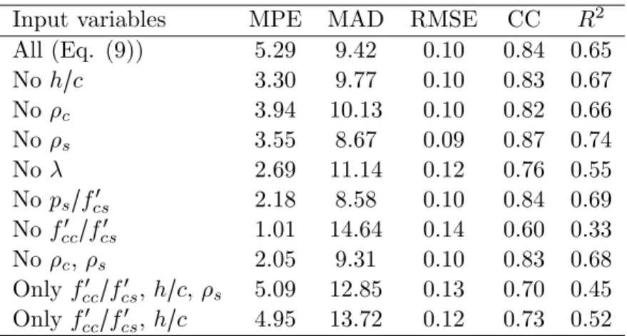
Similarly, Table 4 gives the results of sensitivity analysis for Model-A2. It is apparent that,
fcc′ /fcs′ and l have the most significant effect on normalized effective strength and all other dimensionless variables, namely ρc, h/c, ρs, and ps/fcs′ have the least significant effect. A comparison with the sensitivity analysis of Model-A1, shows that though theh/cratio has little influence on the effective strength of the joint but the slab thickness taken independently has significant effect. The results presented in Tables 3 and 4 indicate that the models incorporating only limited number of the available parameters likefcc′ /fcs′ , andh/care not good enough for achieving the desired accuracy and reliability in predicting the joint effective strength. Eq. (8) was devised using many of the non-dimensional variables and thus resulted in relatively better values of the coefficient of determination and correlation coefficients (R2and CC). These findings are consistent with existing understanding of the relative importance of the various parameters on joint effective strength.
Table 4 Sensitivity analysis of Model A-2 with feed-forward back propagation.
Input variables MPE MAD RMSE CC R2
All (Eq. (9)) 5.29 9.42 0.10 0.84 0.65
Noh/c 3.30 9.77 0.10 0.83 0.67
Noρc 3.94 10.13 0.10 0.82 0.66
Noρs 3.55 8.67 0.09 0.87 0.74
Noλ 2.69 11.14 0.12 0.76 0.55
Nops/fcs′ 2.18 8.58 0.10 0.84 0.69
Nofcc′ /fcs′ 1.01 14.64 0.14 0.60 0.33
Noρc,ρs 2.05 9.31 0.10 0.83 0.68
Onlyfcc′ /fcs′ ,h/c,ρs 5.09 12.85 0.13 0.70 0.45 Onlyfcc′ /fcs′ ,h/c 4.95 13.72 0.12 0.73 0.52
The Model-A1 using the raw variables is found to be better than the Model-A2 involving non-dimensional parameters. The study of sensitivity of Model-A1 gives the impression that elimination of some of the variables has only marginal influence on the resulting joint effective strength. However considering the limitations and uncertainties in the data, a full-fledged network involving all input variables would be desirable.
A.A. Shah et al / Estimation of RC Slab-column joints effective strength using neural networks 405
7 ANALYSIS AND INTERPRETATION OF TEST RESULTS
The preprocessing of the network training set was performed by normalizing the inputs and targets so that they have means of zero and standard deviations of 1. Similarly, all weights and bias values were initialized to random numbers. While the numbers of input and output nodes are fixed, the hidden nodes in the case of FFBP were subjected to trials and the one producing the most accurate results (in terms of the CC) was selected. The optimization of the training procedure automatically fixes the hidden nodes in the case of the CFBP. The training of these networks was stopped after reaching the minimum mean square error between the network yield and true output over all the training patterns.
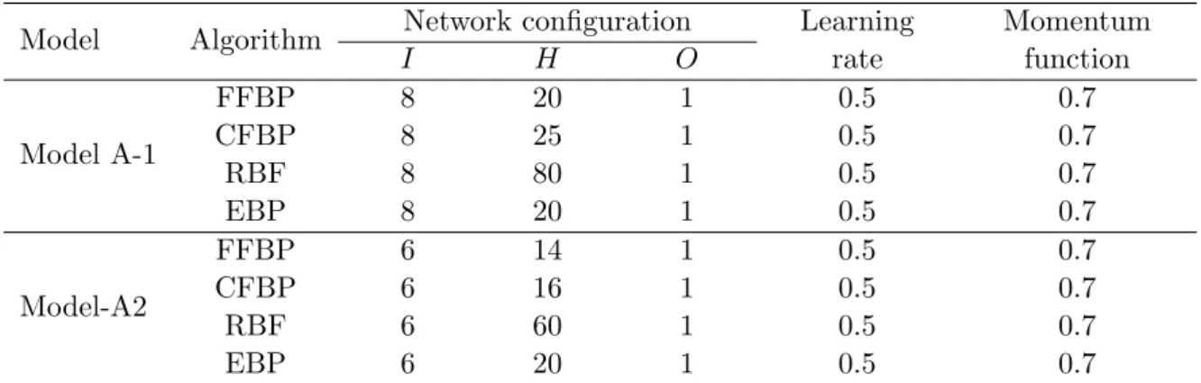
The information on number of nodes required to achieve minimum error taken in the case of each training scheme used (i.e. FFBP, CFBP and EBP) is shown in Table 5 for Model-A1 and A2. As a matter of general information, which is not of real significance in this study, it can be seen that the cascade correlation algorithm, designed for efficient training, trained the network with fewer epochs than the FFBP network.
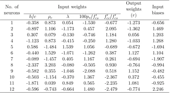
The network architecture of the two models, given by Eqs. (8) and (9), is given in Figs. 2 and 3 respectively for BP training scheme. The error estimation parameters, on the basis of which the performance of a model is assessed, are given in Tables 3 and 4. Training and validation results for the two models are shown in Figs. 4 and 5. The trained values of connecting weights and bias for the two models are given in Tables 6 and 7 obtained from FFBP training scheme.
Table 5 Network architecture.
Model Algorithm Network configuration Learning
rate
Momentum function
I H O
Model A-1
FFBP 8 20 1 0.5 0.7
CFBP 8 25 1 0.5 0.7
RBF 8 80 1 0.5 0.7
EBP 8 20 1 0.5 0.7
Model-A2
FFBP 6 14 1 0.5 0.7
CFBP 6 16 1 0.5 0.7
RBF 6 60 1 0.5 0.7
EBP 6 20 1 0.5 0.7
Note: I,H,O indicate number of input, hidden, and output nodes, respectively; FFBP, feed-forward back propagation; CFBP, cascade-forward back propagation;
RBF, radial basis function; EBP, Elman back propagation network.
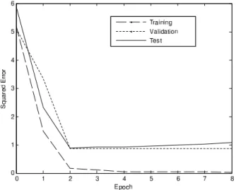
The histograms of error in the prediction of the joint effective strength for Model-A1, which is found to be better than Model-A2, are plotted in Fig. 6. The percentage error in the prediction of the joint effective strength for different data sets is plotted in Fig. 7 for Model-A1. The predicted value of the effective strength of joint has been plotted against its observed value in Fig. 8 for the Model-A1.
406 A.A. Shah et al / Estimation of RC Slab-column joints effective strength using neural networks
Figure 2 Model-A1: use of raw variables.
Figure 3 Model-A2: use of non-dimensional variables.
Figure 4 Epochs versus squared error of raw variables (Model – A1) by back propagation.
A.A. Shah et al / Estimation of RC Slab-column joints effective strength using neural networks 407
Figure 5 Epochs versus squared error of grouped variables (Model – A2) by back propagation.
Figure 6 Histogram of percentage error for Model-A1.
It also shows that the use of raw variables as input (i.e. Model-A1) may be more beneficial than that of the non-dimensional grouped variables (i.e. Model-A2), provided an appropriate training scheme is chosen. The most suitable network, FFBP Model-A1, has the highest CC=0.97 and R2=0.94; and lowest MPE=1.30, MAD=7.90, and RMSE=6.69. All the ANN models featured small RMSE during training; however, the value was slightly higher during validation. The models showed consistently good correlation throughout the training and testing. In conclusion the network configuration (FFBP Model-A1) along with corresponding weight and bias matrix given in Table 6 is recommended for general use in order to predict the effective strength of the joint.
The mean error in the prediction of the joint effective strength by various regression models
408 A.A. Shah et al / Estimation of RC Slab-column joints effective strength using neural networks
Table 6 Connection weights and biases for Model-A1 (refer to Fig. 2) (output bias = 0.6582).
No. of neurons
Input weights Outputweights
(r)
Input biases
h c ρc λ ps fcc′ fcs′
1 0.707 0.512 0.992 -0.833 0.322 -0.724 -1.508 0.971 2.053
2 -0.511 0.269 0.629 1.086 0.205 -0.493 -2.484 1.303 1.962
3 -1.050 -0.199 -0.685 0.693 1.299 -1.322 -0.503 -1.017 2.290
4 -0.003 1.462 0.906 1.946 -0.618 -0.419 0.789 0.339 -1.496
5 0.260 0.328 1.568 -0.953 -1.109 0.767 0.529 -0.181 -1.576
6 0.033 -0.828 -1.114 -1.016 0.865 -2.501 -0.966 -0.237 1.426
7 -0.009 -5E-04 0.468 -0.472 1.072 -1.301 1.202 -1.052 1.019
8 0.006 -0.889 -0.556 -0.488 1.151 0.123 0.501 0.159 -0.976
9 1.032 -0.303 -0.452 -1.037 0.150 -1.025 0.473 -0.053 1.495
10 -0.466 -1.140 -1.530 -0.622 -0.423 0.768 2.033 0.311 -0.425
11 -0.652 -0.353 0.816 -0.531 1.931 0.047 0.990 0.575 1.188
12 -0.187 0.593 1.491 -0.028 -0.480 0.689 -1.413 -2.172 1.190
Table 7 Connection weights and biases for Model-A2 (refer to Fig. 3) (output bias = 0.3827).
No. of neurons
Input weights Outputweights
(r)
Input biases
h/c ρc λ 100ps/fcs′ fcc′ /fcs′
1 -0.358 0.873 0.054 -1.530 -0.677 -1.273 -0.656
2 -0.897 1.106 -1.173 0.457 2.095 -1.362 1.469
3 0.307 0.079 -0.130 -0.746 1.184 0.056 1.203
4 -1.123 0.873 -0.415 -0.250 1.280 -1.033 1.268
5 0.586 -1.484 1.539 1.056 -0.689 -0.672 -1.694
6 -0.440 1.529 -1.071 -1.262 0.387 1.127 1.104
7 -0.089 -1.457 0.405 1.167 0.261 -0.694 -1.907
8 -2.337 3.203 -0.080 -0.505 0.930 -0.764 -0.994
9 -0.582 0.355 -1.046 -2.088 0.518 1.152 -0.482
10 -0.503 -1.154 -0.370 1.367 -2.367 0.372 -0.455
11 -1.871 0.039 0.849 0.565 -2.235 1.081 -0.925
12 -0.596 -0.743 -0.664 1.480 -2.479 -0.774 2.246
A.A. Shah et al / Estimation of RC Slab-column joints effective strength using neural networks 409
(Eq. (1-6)) may be compared with the performance of neural network Model-A1 where the mean error is only 7.4%. On the other hand the mean errors calculated using regression models by Shah and Ribakov [22], Ospina and Alexander [17], ACI [1], and CSA [5] are 18.31, 15.69, 20, and 18.37%, respectively. The histogram of percentage error of a neural network model in comparison with the corresponding histograms for the earlier regression based models [1, 5, 17, 22] given by Eq. (1-6) is shown in Fig. 6. It is observed from this figure that for 72% of the data the percentage error is less than 10% for the neural network model, whereas the percentage error in the regression based models [1, 5, 17, 22] in the same percentage of data is about 25%. Similarly, for 93% of the test data the percentage error for the neural network Model-A1 obtained is less than 25%, while for almost the same percentage of data the regression based models [1, 5, 17, 22] are showing the percentage error as 36%. This clearly indicates the supremacy of the neural network model over the regression models.
Figure 7 Percentage error in prediction of effective strength by Model-A1 for individual data points.
Figure 8 Observed versus predicted effective strength.
410 A.A. Shah et al / Estimation of RC Slab-column joints effective strength using neural networks
8 CONCLUSIONS
A generalized model for predicting the slab-column joint effective strength using neural network (NN) has been developed. The network predictions were generally more satisfactory than those given by traditional regression equations because of low errors and high correlation coefficients. Predictions based on raw data (h, c, ρc, ρs, λ, ps, fcc′ and fcs′ ) were better than those based on the grouped dimensionless form of the data (h/c,ρc,ρs,λ,ps/fcs′ , andfcc′ /fcs′ ).
The NN with one hidden layer was selected as the optimum network to predict the effective strength of joint. The network configuration of Model-A1 with feed-forward back propagation is recommended for general use in order to predict the effective strength of joint.
Sensitivity analysis was performed in order to determine the relative significance of each of the independent parameters (input neurons) on the joint effective strength (output) in both of the NN models that were used in the frame of this study. On the basis of this analysis it was observed that the slab confinement factor, the slab thickness, and the column concrete strength are the three most significant parameters for the prediction of effective strength of the joint. From the study of sensitivity of the two models as well as keeping in view the variability in the outcome resulting from application of different analytical schemes, it is felt that the network which requires all input quantities may be followed for generality. Results of this study demonstrate that the NN model is far better than the regression one because it more precisely determines the effective strength of a column-slab joint and is, therefore, recommended for general use in order to predict the effective strength of the joint.
Acknowledgements The first author gratefully acknowledges the support by the Specialty Units for Safety and Preservation of Structures, College of Engineering, King Saud University, Riyadh, Kingdom of Saudi Arabia.
References
[1] American Concrete Institute (ACI 318-08), Detroit, Michigan. Building code requirements for structural concrete and commentary, 2008.
[2] A. C. Bianchini, R. E. Woods, and C. E. Kesler. Effect of floor concrete strength on column strength. ACI Journal, 31(11):1149–69, 1960.
[3] M. Bilgehan and P. Turgut. The use of neural networks in concrete compressive strength estimation.Computers and Concrete, 7:271–283, 2010.
[4] E. Buckingham. On physically similar systems; illustrations of the use of dimensional equations. Physical Review, 4:345–376, 1914.
[5] Canadian Standards Association (CSA A23.3-94), Rexdale, Ontario, Canada. Design of concrete structures, 1994.
[6] Y. S. Cho, C. J. Seo, and E. S. Kang. A study of flat plate slab-column connections with shear plate in tall concrete building using experimental and numerical analysis. Technical report, Council on Tall Buildings and Urban Habitat (CTBUH), Seoul, Korea, 2004.
[7] V. N. T. Dao, P. F. Dux, and L. O’Moore. Punching shear of slab-column connection in flat-plate construction. InProceedings of International Congress on Global Construction; Ultimate Concrete Opportunities, pages 183–190, Scotland, 2005. University of Dundee.
[8] W. L. Gamble and J. D. Klinar. Tests of high-strength concrete columns with intervening floor slabs.ASCE Journal of Structural Engineering, 117(5):1462–76, 1991.
A.A. Shah et al / Estimation of RC Slab-column joints effective strength using neural networks 411
[9] F. Jungwirth. Knotenpunkt: normalfeste Decke–hochfeste Ortbetonstutze. Leipzig annual journal on concrete and concrete structures, 3(1):165–74, 1998. Leipzig Annual Civil Engineering Report [in German].
[10] T. H.-K. Kang, S.-H. Kee, S. W. Han, L.-H. Lee, and J. W. Wallace. Interior posttensioned slab-column connections subjected to lateral cyclic loading. InProceedings of 8th national conference on earthquake engineering, San Francisco, USA, 2006.
[11] S-J. Kwon and H-W.Song. Analysis of carbonation behavior in concrete using neural network algorithm and carbon-ation modeling. Cement and Concrete Research, 40:119–127, 2010.
[12] M.Y. Mansour, M. Dicleli, J.Y. Lee, and J. Zhang. Predicting the shear strength of reinforced concrete beams using artificial neural networks.Engineering Structures, 26:781–799, 2004.
[13] The MathWorks, Inc., Natick, MA, USA. MATLAB and Simulink for technical computing, 2010.
[14] The MathWorks, Inc., Natick, MA, USA. Neural networks toolbox V6.0.4, 2010.
[15] P. J. McHarg, W. D. Cook, D. Mitchell, and Y. S. Yoon. Improved transmission of high strength concrete column loads through normal strength concrete slabs. ACI Structural Journal, 97(1):157–66, 2000.
[16] H. Naderpour, A. Kheyroddin, and G.G. Amiri. Prediction of frp-confined compressive strength of concrete using artificial neural networks.Composite Structures, 92:2817–2829, 2010.
[17] C. E. Ospina and S. D. B. Alexander. Transmission of interior concrete column loads through floors.ASCE Journal of Structural Engineering, 124(6):602–10, 1998.
[18] R. Perera, M. Barch´ın, A. Arteaga, and A. De Diego. Prediction of the ultimate strength of reinforced concrete beams frp-strengthened in shear using neural networks.Composites: Part B, 41:287–298, 2010.
[19] L. Ran, S. C. Young, and Z. Sumei. Punching shear behavior of concrete flat plate slab reinforced with carbon fiber reinforced polymer rods.Composites: Part B, 38:712–719, 2008.
[20] A. A. Shah, J. Dietz, N. V. Tue, and G. Koenig. Experimental investigation of column–slab joints. ACI Struct J, 102(1):103–13, 2005.
[21] A. A. Shah and Y. Ribakov. Experimental and analytical study of flat-plate floors confinement. Materials and Design, 26(8):655–69, 2005.
[22] A. A. Shah and Y. Ribakov. Using mechanics of materials approach for calculating interior slab-column joints strength. Materials and Design, 29(8):1145–1158, 2008.
[23] J. Sobhani, M. Najimi, A.R. Pourkhorshidi, and T. Parhizkar. Prediction of the compression strength of no-slump concrete: A comparative study of regression, neural network and ANFIS models. Construction and Building Mate-rials, 24:709–718, 2010.
[24] S. Teng. BCA–NTU research on irregular flat-plate structures. Technical report, Department of Civil and Environ-mental Engineering, Nanyang Technological University, Singapore, 1999. Structural Engineering Report.
![Figure 1 Schematic views of slab-columns connection: (a) interior column (b) edge column (c) corner column (d) sandwich column (following [13]).](https://thumb-eu.123doks.com/thumbv2/123dok_br/18884372.423478/3.892.179.665.606.738/figure-schematic-columns-connection-interior-column-sandwich-following.webp)