Lateral strength force of URM structures based on a
constitu-tive model for interface element
Abstract
This paper presents the numerical implementation of a new proposed interface model for modeling the behavior of mor-tar joints in masonry walls. Its theoretical framework is fully based on the plasticity theory. The Von Mises criterion is used to simulate the behavior of brick and stone units. The interface laws for contact elements are formulated to sim-ulate the softening behavior of mortar joints under tensile stress; a normal linear cap model is also used to limit com-pressive stress. The numerical predictions based on the pro-posed model for the behavior of interface elements correlate very highly with test data. A new explicit formula based on results of proposed interface model is also presented to esti-mate the strength of unreinforced masonry structures. The closed form solution predicts the ultimate lateral load of un-reinforced masonry walls less error percentage than ATC and FEMA-307. Consequently, the proposed closed form solution can be used satisfactorily to analyze unreinforced masonry structures.
Keywords
masonry wall, interface element, softening behavior, micro modeling, cap model, tensile strength of mortar joint.
A.H. Akhaveissy∗
Department of Civil Engineering, Faculty En-gineering, Razi University, P.O. Box 67149– 67346, Kermanshah, Iran
Received 25 Apr 2011; In revised form 27 Jul 2011
∗Author email: [email protected]
1 INTRODUCTION
Masonry is the oldest building material that still finds wide use in today’s building industries. Masonry buildings are constructed in many parts of the world where earthquakes occur. Hence, knowledge of their seismic behavior is necessary to evaluate the seismic performance of these types of building. Pushover analysis is commonly used to evaluate seismic performance and to determine the capacity curve. Therefore, the capacity curve is studied in this paper.
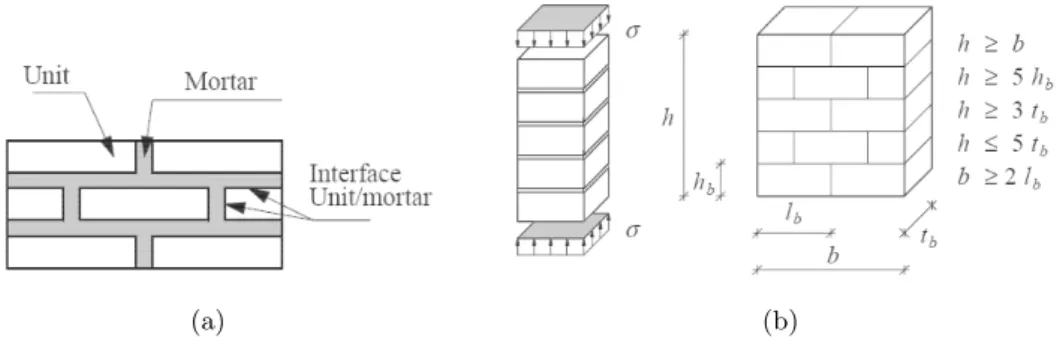
Important new developments in masonry materials and applications have occurred in the past two decades. Masonry is a composite material that consists of block and mortar joints. Hence, micro-modeling is used for the detailed analysis of masonry and may include a repre-sentation of clay bricks, mortar and the block/mortar interface, Fig. 1(a).
(a) (b)
Figure 1 (a) Detailed micro-modeling of masonry, and (b) schematic representation of a test specimen.
mortar to be governed by the Mohr-Coulomb criterion. Thanoon et al. [18] implemented the cohesion-less Mohr-Coulomb criterion to analyze interlocking mortarless block masonry systems. Senthivel and Lourenco [15] implemented the model in [9] to analyze stone masonry shear walls. The obtained results show good agreement with test data. Brasile et al. [2] proposed a coarse-scale model based on an assumed stress finite element formulation. They obtained the nonlinear behavior by assuming a set of planes on the element where the frictional response can take place, together with the tensile and compression limit stress.
In accordance with the research above on the numerical analysis of masonry walls by the use of micro modeling processes, the models can be divided into groups: 1) one group used the tension cut-off model with the compressive cap model for the mortar joint and elastic behavior of a block [7, 13, 18], 2) another group used the tension cut-off model without the compressive cap model for the mortar joint for either the elastic-plastic behavior for block masonry [2, 16] or the elastic behavior for block masonry [6], and 3) the final group implemented the tension cut-off model with the compressive cap model for mortar joints and the elastic behavior of block masonry [4, 8, 9, 11, 15, 17]. Therefore, based on these divisions, it is necessary to investigate masonry walls with the use of the tension cut-off model with the compressive cap model and elastic-plastic behavior for block masonry with a simple formulation. This paper focuses on masonry walls with this aim.
2 THE INTERFACE MODEL
Masonry is a composite material that consists of units and mortar joints. A masonry wall is constructed by laying pieces of bricks on top of each other with cohesion via mortar. The mortar joint can be modeled by interface elements and bricks by isoparametric elements. Sliding on mortar joints may occur for a masonry wall under a lateral force. Modeling of this phenomenon with standard finite elements would lead to numerical ill conditioning due to the high aspect ratios present. The idea of overcoming this problem by introducing special elements is not new [8]. However, in this paper, the joint elements were developed by Giambanco et al. [6] and [2, 16]. Sekiguchi [14] applied 6-noded joint elements in an elasto-viscoplasticity analysis based on tangential and normal stiffness of joint elements related to the force-displacement relationship. Here, a 6-noded joint element is reformulated based on tangential and normal elasticity modules related to the stress-strain relationship, as shown in Fig. 2.
The elastic stiffness matrix of a joint element is defined in the standard finite element as
Ke= ∫ ve
BTDBdV (1)
where the B matrix is defined as
B = 1
wN (2)
The evaluation of Ke in (1) can be performed as a line integral:
Ke=t∫
1
−1
BTDB[(∂x ∂ξ)
2
+ (∂y∂ξ) 2
] 1/2
dξ (3)
where t is width of joint element, and D is the stress-strain matrix in the local coordinate system. The elastic stress-strain relation is defined as
d σ
−={
dτ dσ }=[
ET 0
0 En ] {
dγ dεn }=
Dd ε
−, d ε−=
1 w{
rξ
rη }=
1
wr (4)
Here we note that ET and En are tangential and normal elastic modules, respectively, in the
local coordinates of the joint element, and r is illustrated as
r={ rξ rη }={
topξ−bottomξ
topη−bottomη }=[ −
N1 −N2 −N3 N4 N5 N6 ] ⎧⎪⎪⎪⎪ ⎪⎪⎪⎪⎪ ⎪⎪ ⎨⎪⎪⎪ ⎪⎪⎪⎪⎪ ⎪⎪⎪⎩ a1 a2 a3 a4 a5 a6 ⎫⎪⎪⎪⎪ ⎪⎪⎪⎪⎪ ⎪⎪ ⎬⎪⎪⎪ ⎪⎪⎪⎪⎪ ⎪⎪⎪⎭
=N a
ai={
ui
vi }, Ni=[ ni 0
0 ni ] [
cosθ sinθ
−sinθ cosθ ], θ=tan
−1⎛ ⎝ ∂y/ ∂ξ ∂x/ ∂ξ ⎞ ⎠ (5)
where the shape functions ni associated with node I are expressed in terms of the local ξ
coordinate as
ni= 12ξξi(1+ξξi) i=1,3,4,6
ni= 1−ξ2 i=2,5
(6)
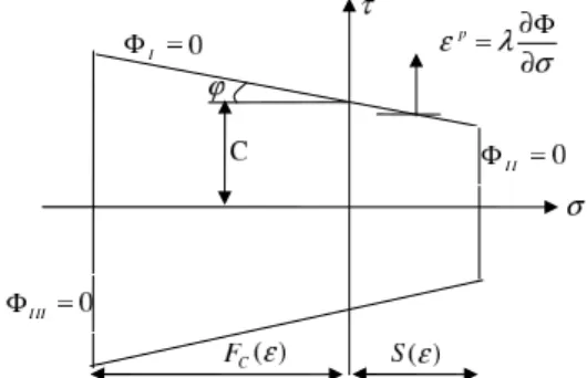
Irreversible discontinuous displacements occur when the stress state reaches a limit condi-tion. In this paper, the elastic domain is defined by three convex limit surfaces intersecting in a non-smooth fashion: the Coulomb criterion for the shear stress state, the tension cut-off for the tensile stress state and the compression cut-off for compressive strength. The limit functions, reported in the stress space, as shown in Fig. 3, take the following form:
ΦI=∣τn∣ +σntanϕ−C=0
ΦII=σn−S(ε)=0
ΦIII =σn+FC(ε)=0
whereϕis the internal friction angle of the contact layer, εis the normal strain,C,S andFC are cohesion, tensile strength and compressive strength of the contact layer, respectively, and σn,τn are the amount of normal stress and shear stress on the interface surface, respectively.
These stresses are calculated in local coordinates.
Figure 3 Yield condition represented in the stress space.
The stresses will be calculated for step n and iteration i+1 based on the amount of stresses in step n and iteration i by use of the elastic predict-plastic correction as
i+1
σ − ∗ n= σ − i n+ dσ −n (8)
By substituting Eq. (8) in Eq. (7), the predicted stresses are found to be
IF ΦI,ΦII,ΦIII ≤0 ⇒σ
−
i+1
n = i+1
σ
− ∗
n
IF ΦII≻0,ΦI<0 or ΦI ≻0 ⇒i+
1
σ
n =s, τ i+1
n =∣−σ i+1
n tanϕ+C∣ i+1
τn∗
∣i+1τ∗
n∣
IF ΦII≤0,ΦI≻0 ⇒
i+1
σ
n = i+1
σn∗, τni+1=∣−σin+1tanϕ+C∣
i+1
τn∗
∣i+1τ∗
n∣
IF ΦIII ≻0,ΦI <0 or ΦI≻0 ⇒i+
1
σ
n =FC, τ i+1
n =∣−σi+
1
n tanϕ+C∣ i+1
τn∗
∣i+1τ∗
n∣
IF ΦIII ≤0,ΦI ≻0 ⇒i+
1
σ
n = i+1
σn∗, τni+1=∣−σin+1tanϕ+C∣
i+1
τn∗
∣i+1τ∗
n∣
(9)
3 FINITE ELEMENT ANALYSIS
joints and units. For this purpose the program was in the FORTRAN language. The Von-Mises criterion was assumed for the behavior of blocks, and the proposed yield/failure surface was applied for the behavior of mortar joints. Three Lobatto points were considered for each contact element, and 2*2 gauss points for the 8-nodes isoparametric elements were used to carry out the numerical integrations. This method and the program were applied for modeling a number of experimental tests, and two examples are considered in the following section.
3.1 Numerical Example
3.1.1 The masonry shear wall example
This example simulates the mechanical response of the masonry wall illustrated in Fig. 4. Experimental tests on a masonry wall were carried out by Vermeltfoort et al. [19]. The wall was made of wire-cut solid clay bricks with dimensions of 210*52*100 mm3
and 10-mm thick mortar joints and characterized by a height/width ratio of one, with dimensions of 1000*990 mm2
. Two stiff steel beams at the horizontal boundaries of the test setup clamp on the top and the bottom wall. The geometry of the model and the boundary conditions adopted are shown in Fig. 4. At the top horizontal side of the wall, the vertical degrees of freedom are constrained using a uniform distribution of springs of stiffness ksimulating the stiffness of the test apparatus [6].
(a) (b)
Figure 4 (a) Solid masonry wall geometry and (b) boundary and loading conditions [5, 14].
The elastic properties of the bricks as well as the joint with the interface parameters characterizing the strength properties are reported in Table 1. Fig. 5 shows the softening behavior of mortar in tension and the behavior of mortar in compression. The behavior of bricks is assumed to be elastic-perfect plastic. The behavior is modeled by the Von-Mises criterion.
Here, E is the elastic modulus, Et the tangential modulus, υ the Poission ratio, Fc the
compressive strength,Ft the tensile strength,C the shear strength andφthe friction angle.
The value of the stiffness k has been previously calibrated to obtain a final collapse of the wall for a slip type mechanism [6]. The value of the stiffness k = 9∗104
Table 1 Properties of brick and mortar joints (in terms of N/cm2 ).
Brick Mortar Joint
E [6] υ [6] Fc Et E [6] υ [6] C [6] φ[6] Fc Ft [6]
1670000 0.15 175 0 78200 0.14 35 37o 150 25
(a) (b)
Figure 5 (a) Compressive and (b) tensile behavior for the mortar joint used in the analysis.
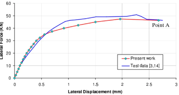
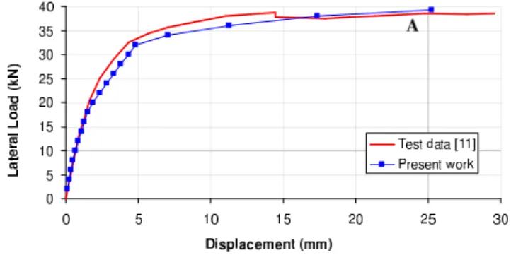
are represented by plane stress continuum elements (8-noded), whereas line interface elements (6-noded) are adopted for the joints. Each brick is modeled with 2*1 elements. The wall is modeled by 160 8-noded isoparametric elements, 222 interface elements and 2086 degrees of freedom. The value of error for the displacement convergence criterion is 1e-5. Fig. 6 shows the comparison between the predicted load-displacement curve and the test data. The comparison expresses significant relation between the predicted results and the test data.
Figure 6 Comparison between test data and predicted load-displacement curve.
Fig. 6 shows that the predicted ultimate load is 93.25% of the observed ultimate load, and that the load-displacement curve obtained from analysis is in good correlation with test data. The shear and tension failure occurred at the bottom of the wall due to a combination of shear force and bending moment. At the top of the wall, the tensile failure occurred in the vertical mortar and shear failure in horizontal mortar. Fig. 7 shows the failure of the wall.
Figure 7 Deformed shape for the last step (Point A from Fig. 6).
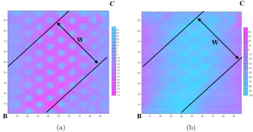
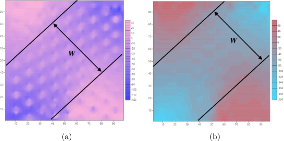
interface elements is shown in Fig. 8, in the same way the variation of normal stress is shown in Fig. 9.
(a) (b)
Figure 8 Distribution of shear stress for a) interface element and b) 8-noded isoparametric element with dimensions in cm and shear stress in N/cm2
.
Fig. 8 shows distribution of the shear stress in the direction of the diagonal of the wall, BC, and the distribution of normal stress is expressed in Fig. 9. In both Fig. 8 and Fig. 9, the width of the compressive diagonal is shown with the parameter W, which is about 60 cm or 40% of the length of the diagonal.
3.1.2 The stone-masonry shear wall example
The irregular stone masonry with bonding mortar is representative of large stone block con-struction, possibly in monumental buildings. The data were obtained from the ancient stone masonry shear wall test [15]. The average compressive strength, tensile strength and Young’s modules of the stone were 69.2 N/mm2
, 2.8 N/mm2
and 20200 N/mm2
, respectively. The average compressive strength of the mortar was 3.0 N/mm2
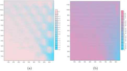
(a) (b)
Figure 9 Distribution of normal stress for a) interface elements and b) 8-noded isoparametric elements with dimensions in cm and shear stress in N/cm2
.
mm (length) * 1200 mm (height) * 200 mm (width), and the height to length ratio was 1.2. The dimensions of the sawn stone used in the wall were 200 mm (length) * 150 mm (height) * 200 mm (width). The monotonic lateral load was carried out with a low axial pre-compression load level of 100 kN (σ0=0.5 N/mm
2
).
(a) (b)
Figure 10 The dimensions of the stone wall: a) the irregular stone wall with bonding mortar, boundary condi-tions and initial loading, and b) modeling of the interface element.
Fig. 11 shows the softening behavior of mortar in tension and the behavior of mortar in compression.
Table 2 Properties of stone units and mortar joints (in N/mm2 ).
Stone unit Mortar Joint
E [15] υ [15] Fc [15] Et E [15] υ [15] C [15] φ[15] Fc [15] Ft
20200 0.2 69.2 0 3.494 0.11 0.1 21.80o 3.0 0.032
(a) (b)
Figure 11 (a) Compressive and (b) tensile behavior for mortar joints assumed in the analysis.
error for the displacement convergence criterion is 1e-4. Fig. 12 shows the comparison between predicted load-displacement curve and test data. The comparison expresses close relationship between the predicted results and test data.
Figure 12 Comparison between test data and predicted load-displacement curve.
The variation of the shear stress for point A from Fig. 12 in the isoparametric elements and interface elements is shown in Fig. 13. The variation of normal stress is shown in Fig. 14 too.
Fig. 13 shows that the maximum shear stress occurred above the diagonal of the wall,BC, which is in accordance with the failure observed in the laboratory [15]. In Fig. 13, the width of the compressive diagonal is shown with the parameterW, which is about 470 mm or 30%
of the length of the diagonal. The maximum normal tensile stress shows the tensile failure of mortar joints and no crushing in the mortar joints due to compressive stress; see Fig. 14.
(a) (b)
Figure 13 Distribution of shear stress for a) interface elements and b) 8-noded isoparametric elements with dimensions in mm and shear stress in N/mm2
.
(a) (b)
Figure 14 Distribution of normal stress for a) interface elements and b) 8-noded isoparametric elements with dimensions in mm and shear stress in N/mm2
.
coefficient by use of parameters in Table 1 was determined for a height/width ratio of two, with dimensions of 100*50 cm2
and the ratio of four, with dimensions of 200*50 cm2
. The thickness of the wall was 10 cm. The coefficient for the ratio two and four was determined 0.22 and 0.12, respectively. Fig. 15 shows variations of the coefficient versus different height/width ratio of the wall. This coefficient is shown byFw.
Figure 15 The coefficient of compressive diagonal versus high to width ratio of wall.
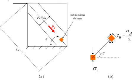
(a) (b)
Figure 16 a) compressive effective width of the wall and b) principal stress on infinitesimal element.
According to Fig. 16, the resistance lateral force is as follows:
P =Pd∗ COS(θ)
Pd= FwLdtσd; σd= 2τu
τu= C+σ0tan(φ)
(10)
where, C and φ are the cohesive strength and the friction angle, respectively. In Eq. (10), σ0 is the initial applied pressure on the top of the wall. The lateral resistance force of two
previous boundary value problems are determined based on Eq. (10), see Table 3.
Table 3 Comparison of prediction by Eq. (10) and test data.
h/L σ0 τU θ Ld Fw t P (kN) Test Error
(mm) (MPa) (MPa) (mm) (mm) Eq. (10) (kN) %
1000
990 0.3 .35+0.754σ0 45.29 1407.2 0.40 100 45.63 50 -8.7 1200
1000 0.5 .10+0.400σ0 50.19 1562.1 0.30 200 36.00 38 -5.3
Table 4 Comparison between estimated ultimate lateral load by proposed method, Eq. (10), test data [10] and ATC [1].
h/L σ0 τU θ Ld Fw t P (kN) Test Error of
present work %
Reference and (reported error in reference)
(mm) (MPa) (MPa) [10] (mm) (mm) Eq. (10) (kN)
2000
1000 0.6 .21+0.81σ0 63.43 2236.1 0.22 250 76.57 72 6.3 [5] (-42.4%) 1350
1000 0.6 .21+0.81σ0 53.47 1680.0 0.28 250 97.44 85 14.6 [5] (-26.0%) 3000
1500 1.24 .14+0.55σ0 63.43 3354.1 0.22 380 206.2 185 11.4 [5] (-33.6%) 2000
1500 0.68 .21+0.81σ0 53.13 2500.0 0.29 380 251.5 227 10.8 [5] (-48.6%)
The ultimate lateral force and error percentage presented by [5] were calculated based on ATC [1]. Table 4 shows that maximum error percentage of predicted lateral resistance force by Eq. (10) was about 15%, however the maximum error percentage from [5] based on ATC [1] was about 49%.
To assess the ability of the proposed formula, Eq. (10), predictions between results by Eq. (10) and ATC and FEMA-307 [1] are compared in Table 5. The thickness for all of the walls in Table 5 is the same as 250 mm.
Table 5 Comparison between predictions by Eq. (10) and ATC (FEMA307) [1].
h/L σ0 τU θ Ld Fw P (kN) Test Error ATC (kN),
(m) (MPa) (MPa) (mm) Eq. (10) (kN) % error%
3
1.5 1.245 .0+0.813σ0 63.43 3354 0.22 167 185 -9.7 275, 48.6
6(f t)
11.42(f t) 93 (psi) 0.0+σ0 27.72 12.9 (ft) 0.64 163 (kips) 157 (kips) -3.8 177 (kips), 12.7
6(f t)
9.5(f t) 141 (psi) 0.0+σ0 32.27 11.2 (ft) 0.58 186 (kips) 164 (kips) 13.4 186 (kips), 13.4
Comparing amount of error between prediction by ATC [1] and Eq. (10) with test data in Table 5 shows that the predictions by Eq. (10) estimate the lateral resistance force well. Therefore, according to Table 3 to 5, Eq. (10) may be used to estimate the lateral resistance force of unreinforced masonry walls instead of expressed formulations in ATC and FEMA-307.
A single-story unreinforced masonry building
Figure 17 Dimensions of the west wall in mm [12].
The compressive strengths of the brick and mortar were 109 and 9.24 MPa, respectively, and the compressive and tensile strengths of the masonry were 22.2 and 0.18 MPa, respectively [12]. These strengths are used here for the numerical analysis of the west wall. The modulus of elasticity of the masonry specimen was assumed to be 850 times the compressive strength of the masonry specimen [3, 12]. The thickness of the wall was 190 mm. The gravity load, 2.4 kN/m2
, was applied on the diaphragm, whose dimensions were 4091 mm * 5610 mm. Ten wood joists were applied to the diaphragm to transmit the gravity load to the west and east walls. The net span of the wood joist was 5310 mm [12]. Therefore, the gravity load on each wall was 6.37 kN/m.
The Drucker-Prager criterion is used to determine the cohesion strength and the friction angle of the mortar joints. As it is observed from Fig. 7, the failure of the mortar joint usual is occurred in tension. Hence the tensile strength of mortar joints, i.e. 0.18 MPa, is used to calculate the cohesion strength and the friction angle. Therefore, an infinitesimal element is analyzed under shear stress by the Drucker-Prager Criterion to determine these parameters. It is noticeable that the principle stress in principle stresses space in solid mechanics was the same as the shear stress if applied stress on the element was only shear stress. Therefore, loading on the element level is selected to be only shear stress as cyclic loading. Fig. 18 shows shear stress – shear strain curve of the element under cyclic loading for the cohesion strength and the friction angle equal to 0.078 MPa and 31.9 degree, respectively.
Fig. 18 shows the ultimate shear stress for element level and maximum principal normal stress is 0.18 MPa for the cohesion strength and the friction angle equal to 0.078 MPa and 31.9 degree, respectively. It follows that, these parameters are used to determine ultimate base shear of the building by Eq. (10). Hence, the shear strength for piers is determined in accordance with the compressive diagonal region, Fig. 19.
The shear strength for all piers is calculated in Table 6 in accordance with Fig. 19. The initial applied vertical stress on the top of the east wall by dividing uniform load to the thickness is 0.0335 MPa. The ultimate shear stress is calculated based on Eq. (10) is as:
Figure 18 Shear stress – shear strain curve by Drucker-Prager criterion.
Figure 19 Compressive diagonal regions for determination of the ultimate shear force. Table 6 Predicted shear strength by Eq. (10).
Name of pier
h/L θ Ld Fw P (kN)
(mm) (mm) Eq. (10)
Window 953
578 58.76 1114 0.255 5.45
Central 2184
1410 57.15 2599 0.265 13.81
Door 2184
883 67.98 2355 0.198 6.47
∑ 25.73
4 CONCLUSION
The paper presents the numerical implementation of a new proposed interface model for mod-eling the mechanical response of mortar joints in masonry walls. The interface laws are for-mulated in the framework of elasto-plasticity for non standard materials with softening which occurs in mortar joints due to applied shear and tensile stresses. Its theoretical framework is fully based on the plasticity theory. The finite element formulation is based on eight noded isoparametric quadrilateral elements and six noded contact elements. The Von Mises criterion is assumed to simulate the behavior of the units. The interface laws for contact elements are formulated to simulate the softening behavior of mortar joints under tensile stress; a normal linear cap model is also used to limit compressive stress. The capabilities of the interface model and the effectiveness of the computational procedure are investigated by making use of numerical examples that simulate the response of a masonry wall tested under shear in the presence of an initial pre-compression load. Experimental results are provided in the litera-ture to compare with numerical analysis results. The computer predictions correlate very well with the test data. The predicted ultimate load of the masonry wall is estimated to be about 93.25% of the ultimate load according to the test data. The width of the compressive diagonal is about 40% of the length of the diagonal. The proposed model is applied to simulate a stone masonry shear wall. The predicted load-displacement curve is in accordance with the observed data, and diagonal failure is predicted with the use of the distribution of stresses in the stone masonry wall. The width of the compressive diagonal for stone masonry shear wall is about 30% of the length of the diagonal. In addition, a closed form solution was proposed based on the solid mechanics and the compressive effective width of the wall. The closed form solution is better than ATC and FEMA-307 in which predicts the ultimate lateral load of unreinforced masonry walls relatively well. Then it can be concluded that the proposed close form solution can be used satisfactorily to analyze masonry structures similar to those considered herein.
References
[1] Applied Technology Council (ATC).Evaluation of earthquake damaged concrete and masonry wall buildings. Federal Emergency Management Agency, Washington (DC), 1999. Technical Resources.
[2] S. Brasile, R. Casciaro, and G. Formica. Finite element formulation for nonlinear analysis of masonry walls.Computers and Structures, 88:135–143, 2010.
[3] Canadian Standard Association (CSA), Ontario, Canada. Design of masonry structures, 2004.
[4] K. Chaimoon and M. M. Attard. Modeling of unreinforced masonry walls under shear and compression.Engineering Structures, 29:2056–2068, 2007.
[5] S. Y. Chen, F. L. Moon, and T. Yi. A macro element for the nonlinear analysis of in-plane unreinforced masonry piers.Engineering Structures, 30:2242–2252, 2008.
[6] G. Giambanco, S. Rizzo, and R. Spallino. Numerical analysis of masonry structures via interface models. Comput. Methods Appl. Engrg., 190:6493–6511, 2001.
[7] M. Gilbert, C. Casapulla, and H. M. Ahmed. Limit analysis of masonry block structures with non-associative frictional joints using linear programming.Computers and Structures, 84:873–887, 2006.
[9] P. B. Loureno. Computational strategies for masonry structures. Thesis Delft University of Technology. Delft University Press, 1996.
[10] G. Magenes and G. M. Calvi. In-plane seismic response of brick masonry walls. Earthquake Engineering and Structural Dynamics, 26:1091–1112, 1997.
[11] D. V. Oliveira and P. B. Lourenco. Implementation and validation of a constitutive model for the cyclic behaviour of interface elements. Computers and Structures, 82:1451–1461, 2004.
[12] J. Paquette and M. Bruneau. Pseudo-dynamic testing of unreinforced masonry building with flexible diaphragm. Journal of Structural Engineering (ASCE), 129(6):708–716, 2003.
[13] J. R. RIDDINGTON and N. F. NAOM. Finite element prediction of masonry compressive strength. Computers & Structures, 52:113–ll9, 1994.
[14] K. Sekiguchi, R. K. Rowe, K. Y. Lo, and T. Ogawa. Time step selection for 6-noded nonlinear joint element in elasto-viscoplasticity analysis. Computer and Geotechnics, 10:33–58, 1990.
[15] R. Senthivel and P. B. Louren¸co. Finite element modelling of deformation characteristics of historical stone masonry shear walls. Engineering Structures, 31:1930–1943, 2009.
[16] B. Shieh-Beygi and S. Pietruszczak. Numerical analysis of structural masonry: mesoscale approach. Computers and Structures, 86:1958–1973, 2008.
[17] D. J. Sutcliff, H. S. Yu, and A. W. Page. Lower bound limit analysis of unreinforced masonry shear wall.Computers and Structures, 79:1295–1312, 2001.
[18] W. A. Thanoon, A. H. Alwathaf, J. Noorzaei, M. S. Jaafar, and M. R. Abdulkadir. Nonlinear finite element analysis of grouted and ungrouted hollow interlocking mortarless block masonry system.Engineering Structures, 30:1560–1572, 2008.
[19] A. T. Vermeltfoort, T. M. J. Raijmakers, and H. J. M. Janssen. Shear test on masonry walls. InProc. 6th North

![Table 4 Comparison between estimated ultimate lateral load by proposed method, Eq. (10), test data [10]](https://thumb-eu.123doks.com/thumbv2/123dok_br/18884415.423481/13.892.85.759.321.437/table-comparison-between-estimated-ultimate-lateral-proposed-method.webp)
