Lat. Am. j. solids struct. vol.11 número1

(1)

Abs tract

The application of equal displacement rule simplifies the evalua-tion of lateral displacement demand forSDOF system. For complex multi-degree-of-freedom (MDOF) structures such as continuous bridge systems, however, it requires more investigations. In this paper, a comprehensive parametric study of the ratio of maximum inelastic displacement to maximum elastic displacement for typical continuous bridges is performedto advance the application of equal displacement rule to MDOF systems. Particurlarly for the bridges with long periods, this adapted methodlogy is further simplified. It is concluded that equal displacement rule of MDOF is applicable to continuous bridges when the periods of the main modes are no less than the limiting period, which usually serves as an indication to the level of inelastic deformation for a bridge subjected to an earthquake.

Key words

Equal displacement rule, limiting period, continuous bridges, sim-plified seismic analysis, displacement demand

Lateral vibration analysis of continuous bridges

utiliz-ing equal displacement rule

1 INTRODUCTION

The performance-based seismic design philosophy has been sufficiently developed to design a struc-ture system to withstand a pre-defined level of damage under a pre-defined level of earthquake in-tensity. Displacement-based seismic design is an efficient and accurate method to achieve the per-formance-based seismic design philosophy, and it has been proposed and developed in recent years (Kowalsky, 2002; Jameel, Islam, Hussain, et al., 2013). In this methodology, the displacement de-mand of the designed structure should be close to the target displacement, which reflects the pre-defined level of damage of earthquake intensity. Therefore, to obtain the displacement demand of structure is an important step. Although analytical methods are widely utilized to calculate the displacement demand of structure, the analysis processes of currently available methods are rela-tively complex (Chopra and Goel, 2002; Wei, 2011; Akhaveissy, 2012). Hence, it is desired to devel-op a simplified method herein to obtain the displacement demand to facilitate displacement-based seismic design.

B ia o W ei a Y e X i a b,* W e ia n L iu c

a_{School of Civil Engrg., Central South}

Uni-versity, Changsha, China

b_{Dept. of Civil & Environ. Engrg., Rutgers,}

The State University of New Jersey, Piscata-way, NJ 08854, USA

c_{Dept. of Strut. Engrg., Univ. of California,}

San Diego, CA 92093, USA

Received in 21 Nov 2012 In revised form 08 May 2013

(2)

Latin American Journal of Solids and Structures 11(2014) 075 - 091

Equal displacement rule is considered to be an efficient and accurate mechanism to estimate the displacement demand for elastoplastic SDOF systems (Clough and Penzien, 2003; Bayat and Abdol-lahzadeh, 2011). For elastoplastic SDOF structure, which generally satisfies equal displacement rule, the inelastic displacement demand obtained by Nonlinear Time History Analysis (NTHA) is very close to the elastic displacement demand obtained by Response Spectrum Analysis (RSA). Hence, the elastic displacement demand can represent the true elastoplastic displacement demand, resulting in the simplified calculation process of displacement-based seismic design.

Traditional equal displacement rule is considered applicable to SDOF structures when the ac-cording fundamental period is not less than a defined value (Clough and Penzien, 2003). In recent years, equal displacement rule has been further developed and more factors are taken into consider-ation. Efforts are dedicated since 1960s to propsing and studying a displacement correction factor

C, which is equal to the ratio of the maximum inelastic displacement to maximum elastic

dis-placement for SDOF systems subjected to seismic excitation (Veletsos and Newmark, 1960; New-mark and Hall, 1969; Riddell et al. 1989; Miranda, 2000). Therefore, maximum inelastic displace-ment could be approximately obtained by multiplying its elastic counterpart by the factorC.

De-spite of the inconsistent expressions in different literatures, C is approximately equal to 1 for when

the target SDOF has a long fundamental period.This finding is definedas to equal displacement rule. In essence, the previous researches, however, are aimed at investigating SDOF or equivalent SDOF systems. There is little reported study focusing on the lateral deformation of continuous bridges, particularly for irregular bridges with significant higher modes (Isakovic and Fischinger, 2006). In addition, the elastoplastic displacement demand of NTHA is often found to be close to the elastic displacement demand of RSA during traditional seismic design of some continuous bridges. Therefore, it is necessary to study whether the equal displacement rule is still applicable to the MDOF systems.

The objective of this paper is to quantify the application conditions of the equal displacement rule in MDOF bridge systems through a comprehensive parametric study on the ratio of maximum inelastic to elastic displacement in transverse direction for typical continuous bridges. The applica-tion of equal displacement rule simplifies the evaluaapplica-tion of lateral displacement demand of many continuous bridges subjected to earthquakes and provides the basis for their simplified displace-ment-based seismic design.

2 EQUAL DISPLACEMENT RULE OF SDOF

In effort to extend equal displacement rule from SDOF to MDOF system, two key parameters affecting equal displacement rule of SDOF system are introduced accordingly: i) the displacement correction factor C, and ii) the limiting period T_l.

There are many expressions available for the displacement correction factor, and the equation of displacement correction factor C from Miranda (2000) is validated to have better precision by

some researchers and is given by

0.8 1 1

[1 ( 1) exp( 12 )]

C T_µ

µ

− −

(3)

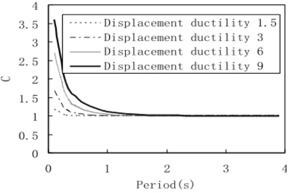
where T is the period of SDOF, µ is its displacement ductility demand. Figure 1 provides the

development of C in terms of T for different µ scenarios, 1.5, 3.0, 6.0,and 9.0respectively,. In this

study, the structural damage level is related to µ, where values (from low to high) approximately

indicate the slight damage state, the moderate damage state, the severe damage state, and the collapse state respectivelyfor reinforced concrete piers of continuous bridges (Xia et al. 2013). As observed from Fig.1, factor C is approaching to 1 as period _T elongates irrespective of

displacement ductility. Note that the limiting period Tl that divides the region where the equal

displacement rule is not applicable from the region where this approximation is applicable de-pends on the level of ductility. In general, Tl increases as µ increases. If C is equal to 1, it is the

rigorous equal displacement rule, however, the value of Tl will be too large and the corresponding

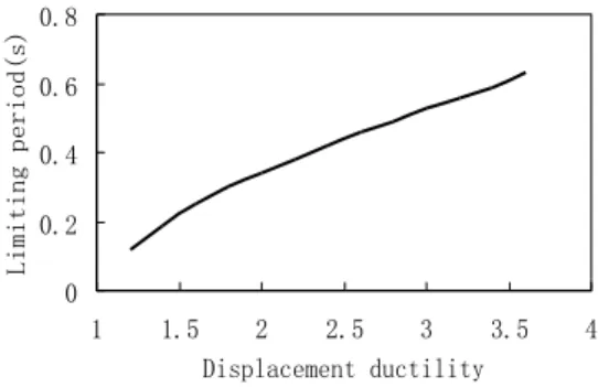
equal displacement rule will not applicable to any structures. Note that the error of 5% is norna-lly acceptable for seismic design. When C is equal to 1.05, equal displacement rule is

approxima-tely considered appropriate, and the correlation between T and µ is shown in Fig.2. Through

curve-fitting process, the equation of the limiting period Tl is determined by

0.4529 ln 0.0323 l

T ₌

_µ

₊ ₍₂₎

When the period T of SDOF is not less than Tl, equal displacement rule is satisfied. As

oppo-sed to the traditional equal displacement rule (Clough and Penzien, 2003), the limiting period Tl

herein is not a constant value, and it is highly dependent on different levels of structure ductility demand. Therefore, the traditional equal displacement rule could be treated as a special case of Eq.(2), which will be thoroughly presented in the following section. Note that equal displacement rule is based on C is equal to 1.05, and equal displacement rule will be more rigorous if C is less

than 1.05.

Figure 1 Crelated to different period and displacement ductility of SDOF 0

0.5 1 1.5 2 2.5 3 3.5 4

0 1 2 3 4

Period(s)

C

(4)

Figure 2 Limiting period of equal displacement rule of SDOF

3 EQUAL DISPLACEMENT RULE OF CONTINUOUS BRIDGES

The objective of this section is to present the results of a comprehensive statistical study of the ratio of maximum inelastic displacement to maximum elastic displacement for typical continuous bridges subjected to earthquakes in the transverse direction, and thus to extrapolate equal displa-cement rule of SDOF to MDOF.

3.1 Typical continuous bridge structures

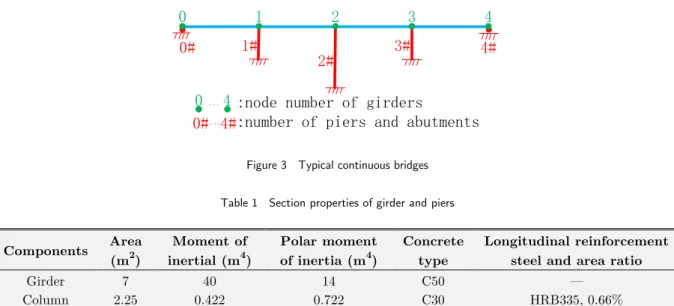
The continuous bridges are widely used in highway and railway [16-17]. Figure 3 provides a 4×

40m continuous bridge configuration with girder and column section properties listed in Table 1. Multi-bearings are laterally set on the top of each column and abutment. Bearings on columns and abutments are all laterally guided except for one laterally fixed on the side column. The arrangement of bearings, which is widely adopted in practical bridge design, prevents abutments with poor ductility from severe earthquake damage.

The displacement ductility demand

µ

e of pier is given by

e e

y

µ = Δ

Δ (3)

In Eq.(3), Δe is the elastic displacement of pier obtained by elastic analysis method, i.e.,

res-ponse spectrum analysis (RSA), while _Δ_y is the yield displacement of pier assumed as one canti-lever column.

Note that, as for bridges with piers of different heights, the moment exists at the top of pier due to the inconsistent deformation of piers and the restriction of girder, therefore, _Δ_y obtained by assuming each pier as one cantilever column may be not the true yield displacement. In addi-tion, Δe may be not the true displacement (approximately true displacement when the structure

satisfies equal displacement rule). Therefore, µe is called nominal displacement ductility demand. 0

0.2 0.4 0.6 0.8

1 1.5 2 2.5 3 3.5 4 Displacement ductility

(5)

0 1 2 3 4

0# 3# 4#

2# 1#

...

0 4

0#...4#

:node number of girders

:number of piers and abutments

Figure 3 Typical continuous bridges

Table 1 Section properties of girder and piers

Components Area (m2)

Moment of inertial (m4)

Polar moment of inertia (m4)

Concrete type

Longitudinal reinforcement steel and area ratio

Girder 7 40 14 C50 —

Column 2.25 0.422 0.722 C30 HRB335, 0.66%

3.2 Earthquake excitation

Earthquake load adopts elastic response spectrum for soil profile III in Chinese criteria (JTJ 004-89 as shown in Fig.4 (Yang et al. 19004-89). It can be used for RSA to obtain the elastic displacement of structures.

Based on the elastic response spectrum, seven artificial motions are generated by Simqke pro-cedure as for ground motion input of NTHA to obtain the inelastic displacement of structures (Fahjan and Ozdemir, 2008), and the average results of NTHA are regarded as the benchmark for comparison with RSA. One representative ground motion out of seven is shown in Fig.5. Other motions are not presented due to the similarity to Fig. 5.

(6)

Figure 5 Ground motion time history (PGA=1.1g) of soil type III

3.3 Analyzing procedure

As for continuous bridges, Tl can be obtained by substituting the maximum nominal

displace-ment ductility demand

µ

em of piers into Eq.(2). The phenomenon, that the displacement

obtai-ned from NTHA is very close to that of RSA when the minimum period _T_min of main modes is no less than the foregoing Tl, is often found in traditional design. The following sections is targeting

to validate this phenomenon.

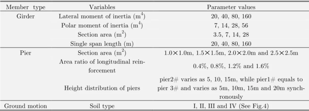
Three cases of continuous bridges with various piers height combinations are identified as the baseline configuration, where shapes and section properties of girders and piers are shown in Fig.3 and Table 1 respectively. Heights of piers of these cases are chosen as 5m-10m-5m, 10m-5m-10m and 5m-5m-5m respectively. Based on the three cases, some parameters are subjected to change to consider more combinations as shown in Table 2, and the combination rule is that one parame-ter is changed by keeping the others the same. As the three cases are the simplified model of the real bridges, the new models of Table 2 obtained by changing only one parameter are reasonable to include many practical bridges, and can be used for numerical simulation.

Table 2 Changing parameters of girder, piers and ground motion

Member type Variables Parameter values

Girder Lateral moment of inertia (m4) 20, 40, 80, 160

Polar moment of inertia (m4) 7, 14, 28, 56

Section area (m2) 3.5, 7, 14, 28

Single span length (m) 20, 40, 80, 160

Pier Section area (m2) 1.0 1.0m, 1.5_×1.5m, 2.0 2.0m and 2.5 2.5m

Area ratio of longitudinal

rein-forcement 0.4%, 0.8%, 1.2% and 1.6%

Height distribution of piers

pier2# varies as 5, 10, 15m, while pier1# equals to pier 3# and varies as 5m, 10m, 15m and 20m

synch-ronously

Ground motion Soil type I, II, III and IV (See Fig.4)

Based on table 2, a majority of cases are identified as irregular bridges which are mainly con-trolled by at least two main modes, and some other cases belong to regular bridge configuration

-15 -10 -5 0 5 10

0 10 20 30 40

( )

t s

2

(/

)

am

s

(7)

which is governed soley by the fundamental mode. Regardless of irregular bridges or regular brid-ges, the sum of main modes participation mass factors of each model should be not less than 90% when dynamic analysis is performed, otherwise the corresponding results of RSA will not be reasonable. Furthermore, the minimum period of the main modes, the sum of whose participation mass factors is just beyond 90%, is defined to be _T_min.

As for each scenario, two different analysis methods are implemented as follows:

(1) RSA was performed by using Opensees software (Mazzoni et al. 2007) with the piers simula-ted by elastic element, and the pier’s initially elastic stiffness adopts the equivalent stiffness. (2) NTHA was also conducted in Opensees analyzing program, in which the piers are simulated by fiber element, where the concrete is simulated by material Concrete02 and the steel is simula-ted by material Steel02.

3.4 Numerical results

For each bridge model, the peak ground acceleration (PGA) need to be adjusted accordingly to ensure the target

µ

em as of being 1.5, 3.0 and 6.0. As for each

µ

em and girder node of bridge cases

shown in Fig.3, the displacement correction factor C is calculated through dividing the

displace-ment of NTHA by the displacedisplace-ment of RSA, and is summarized in scatter plots as shown in Fig.6. Since each bridge has five girder nodes as shown in Fig.3, there are five black dots of C

accor-ding to one _T_min, which is the minimum period of the main modes for one bridge. In case of symmetry, two black dots of C will be covered by the corresponding symmetrical dots, and only

three black dots of C can be seen in Fig.6 according to one

min

T .

As for each

µ

em, T_min is substituted into Eq.(1) to obtain the displacement correction factor C,

and the curve of C is expressed by red line as shown in Fig.6, which is used to judge if it can

capture the distribution features of black dots of C.

In addition, the limiting period Tl of equal displacement rule is obtained by substituting

µ

em

into Eq.(2), and is expressed by green line as shown in Fig.6. As for each

µ

em, the green line of l

T _{divides the black dots of}C into two groups, including the left group wherein

min

T is less than

l

T , and the right group in which

min

T is larger than Tl. The green line of Tl helps to examine

what the dispersion of the black dots of C is relative to 1.0 when

min l

T _≥T .

Characteristics of the irregular continuous bridges regarding the maximum nominal displace-ment ductility demand

µ

em, the displacement correction factor C, the minimum period T_min of

main modes and the limiting period Tl can be observed and summarized from Fig.6 as follows:

(1) For each

µ

em, despite of the dispersion of the black dots of C, the associated C curves in Fig.

6 (a), (b), and (c) is able to capture the distribution features of the black dots of C, which

veri-fies that Eq.(1) of C is meaningful and useful, and Eq.(2) of

l

T obtained by Eq.(1) is reasonable.

(2) For the same

µ

em, the dispersion of the black dots of C relative to the curve of C increases,

(8)

C increases, as

em

µ

increases. Therefore, the distribution of the black dots of C mainly depends

on _T_minand

µ

em, and the influence of other factors is relatively small and can be neglected.

(3) For each

µ

em, most of the black dots of C lie between 0.8 and 1.2 when T_min is not less than

the associated Tl, and the number of the black dots of C beyond the range increases as

µ

em

in-creases.

The abovementioned characteristics show that equal displacement rule is still applicable to the MDOF continuous bridges in the transverse direction when _T_min is not less than Tl, and is

defi-ned as equal displacement rule of MDOF.

(a).

µ

em=1.5

(b).

µ

em=3.0

(9)

Latin American Journal of Solids and Structures 11(2014) 075 - 091 Figure 6 Distribution map of displacement correction factor

c

As equal displacement rule of MDOF is based on the analyses, for all of the continuous bridges with T_min≥Tl, the calculation precisions of equal displacement rule of MDOF are different. Fig.5

shows that as the minimum period _T_min of main modes increases and the displacement ductility demand

µ

em decreases, the displacement correction factor C of each bridge is closer to 1.0, and

the changing trend is gradual. Therefore, it is some arbitrary to select T_min≥Tl as the application

condition of equal displacement rule of MDOF. As for all bridges with T_min≥Tl, if T_min is more

larger than Tl, the calculation precision of equal displacement rule of MDOF will be better,

con-trarily will be worse.

Furthermore, when one structure enters into some level of ductility, the subtle change of the experimental model will produce obviously different displacement. In fact, any analytical methods won’t be able to accurately predict the real elastoplastic displacement, including RSA, ITHA, and other methods. However, the results of these theoretical methods can envelop the possible displa-cement response of the structure. Therefore, as for the seismic design of the structure, especially when the structure’s ductility demand is relatively high, it is unnecessary to pay excessive atten-tion to the calculaatten-tion precision of the theoretical methods. To this extent, the calculaatten-tion errors of equal displacement rule of MDOF are not highly sensitive.

4 EQUAL DISPLACEMENT RULE OF BRIDGES WITH LONG PERIODS

Section three has extended equal displacement rule of SDOF to MDOF. Previous section shows that the limiting period Tl is only related to the maximum nominal displacement ductility

de-mand

µ

em of piers. If

µ

em is substituted by the displacement ductility capacity µΔ of piers, the

derivedTl corresponds to the maximum value related to the maximum allowable level of damage

of one bridge. Therefore, , equal displacement rule can be applied to any allowable level of dama-ge of the briddama-ge provided that T_min≥Tl . As for the piers of general continuous bridges, this

sec-tion will discuss the maximum allowable damage level, and identify the maximum envelop Tl₁ of

the limiting period Tl. Finally, as for the long period bridges, this section will simplify the

appli-cation of equal displacement rule of MDOF.

4.1 Exact formulation of the displacement capacity of piers and the limiting period

In terms of the general continuous bridges, the shortest pier’s displacement ductility capacity µ_Δ

is usually the largest, and thereby it controls the determination of Tl. As the height of the

shor-test pier of one bridge increases, its displacement ductility capacity µ_Δ and the associated Tl in

Eq.(2) decreases, and moreover, _T_minof the bridge increases accordingly. If T_min ≥Tl, equal

(10)

Latin American Journal of Solids and Structures 11(2014) 075 - 091 2

1

3 y

φ

yH

Δ = (4)

in which H is the height of pier, φy is the yield curvature of pier’s section and it can be

calcula-ted by (Tang et al. 2008 ; Kowalsky, 1997)

y y

a

D

ε

φ

= (5)

where D is the section height in the calculated direction of pier, εy is the yield strain of

longitu-dinal reinforcement, the shape factor a is 2.213 for circular section and 1.957 for rectangular

sec-tion.

The displacement capacity Δu is expressed as (Tang et al. 2008):

2 1

( ) ( 0.5 ) / 3

u

φ

yH

φ

u

φ

y Hp H Hp K

Δ = + − − (6)

where H_p is the equivalent analytical plastic hinge length, K is the safety factor of ductility, and φu is the ultimate curvature capacity of pier’s section evaluated by (Kowalsky, 1997)

1 2

( )

c u

D b b

ε

φ

γ

=

+ (7)

in which γ is the axial compression ratio of pier’s section; b₁ and

2

b are shape factors, which are

equal to 0.162 and 0.665 for circular section, and 0.1094 and 0.829 for rectangular sectionrespecti-vely; εcis the ultimate compression strain of concrete shown as (Tang et al. 2008)

' 1.4 0.004

'

s yh su

c

cc f

f

ρ

ε

₌ ₊ (8)

where ' su

ε

_{is the ultimate tensile strain of stirrup with a typical value of 0.09,}

s

ρ is the ratio of volume of stirrup to the core volume of concrete, f_cc_' is the confined compressive strength of

concrete, f_yh is the yield stress of stirrup.

p

H , in Eq. (6), is the least value of the two equations followed by (Tang et al. 2008)

0.08 0.022 0.044

p y s y s

H = H+ f d ≥ f d (9)

min

2

3

p

(11)

where f_y is the yield stress of longitudinal reinforcement, ds is the bar diameter of longitudinal

reinforcement, _D_min is the least cross sectional dimension of pier.

Combing those equations, the displacement ductility capacity µ_Δ of pier can be expressed by

2

1

( ) ( 0.5 ) / ₃

3 ₁ ₍ ₁₎ _{(1 0.5} ₎

1 3

y u y p p

p p

u u

y y

y

H H H H K _H _H

K H H

H

φ φ φ _φ

µ φ φ Δ + − − Δ = = = + − − Δ (11)

Since Eq.(9) is generally applicable to any continuous bridges, substituting Eq.(5), (7) and (9) into Eq.(11) makes

1 2

0.022 0.011 3

1 ( 1)(0.08 )(0.96 )

( )

y s y s

c y

f d f d

K a b b H H

ε

µ

ε

γ

Δ= + − + −

+ (12)

substituting Eq.(5), (7) and (10) into Eq.(11)

min min

1 2

3 2

1 ( 1) (1 )

( ) 3 3

c y

D D

K a b b H H

ε

µ

ε γ

Δ= + − −

+ (13)

Eq.(12) represents the displacement ductility capacity of pier in which H_p is controlled by H, and is applicable to the bridges with dumpy piers. Eq.(13) represents the displacement ductility capacity of pier in whichH_p is governed by _D_min, and is applicable to the bridges with slender

piers. Substituting Eq.(12) or (13) into Eq.(2)

0.4529ln 0.0323 l

T

_µ

Δ

= + (14)

Eq.(14) represents the limiting period of equal displacement rule when the piers are subjected to the damage level of maximum allowable inelastic deformation. To be conservative, the parame-ters in Eq.(12), (13) and (14) need to be analyzed and chosen such that Tl could be achieved as

large as possible, and Tl₁ provides the boundary of Tl. Therefore, all the general continuous

brid-ges under the condition that T_min≥Tl₁ satisfy equal displacement rule.

4.2 Analyzing procedure

In order to ensure the largest possible value of Tl, it is adviced to choose the parameters in

Eqs.(12-14) as follows:

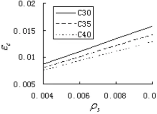
(1) In Eq.(8), stirrup usually uses R235 with the ratio ρs between 0.004 and 0.01 (Tang et al.

(12)

Fig.7. Based on Eqs.(12-14), Tl increases as

ε

c increases. As to obtain large value of Tl,

ε

c can

conservatively adopt 0.015 in structural designs.

(2) Based on Eqs.(12-14), Tl increases as γ decreases, and γ can conservatively adopt 0.1 in

analysis.

(3) The longitudinal reinforcement usually uses HRB335 with ds between 0.016m and 0.038m. ds

adopts 0.028m temporarily in analysis, and will be further discussed in the following text. (4) in particular, K is set to 2.0 according to Chinese criteria (Tang et al. 2008).

Figure 7 The ultimate compression strain εc influenced by concrete strength and the ratio ρs

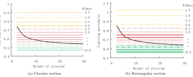
For a typical bridge structure, where _H ranges from 2.5m to 30mand H D/ min is between 2.5

and 10, the developing trend of limiting period

T

l in terms of pier height is depicted in Fig. 8,

considering two different pier cross section, namely cicular and retangular. In this figure, the black curve represents the relations between Tl and H as appeared in Eqs.(12) and (14), and the

color lines represent the relations between Tl and H D/ min indicated in Eqs.(13-14). From Fig.8,

some observations are concluded as follows: (1) Tl decreases, as H and H D/ min increase.

(2) When H D/ min≤4.0, the color lines are all located above the black curve, and Tl is

contro-lled by _H; for H D/ min≥8.0, the color lines are all below the black curve, and Tl is governed by

min

/

H D ; for 4.0<H D/ min<8.0, the color lines and the black curve are crossed, and Tl may be

controlled by H or H D/ min, which depends on the value of H and H D/ min.

Note that the foregoing dividing point of H D/ min is based on ds=0.028m, and will be

diffe-rent for other ds. However, in spite of ds, the maximum value of Tl is always controlled by H,

and is obtained when

γ

and H are the least. In Fig.8, when

_γ

₌0.1 and H₌2.5m, the maximum

value of Tl adopts 0.74s for the circular section of pier, and 0.84s for the rectangular section of

(13)

(a) Circular section (b) Rectangular section

Figure 8 The relations between Tl and H, and between Tl and H D/ min

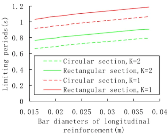
4.3 Numerical results

The previous discussion shows that for the general continuous bridges, when

_γ

₌0.1 and 2.5

H₌ m,

l

T will attain the maximum value, and will be subjected to changes as

s

d varies. Its

relationship is shown in Fig.9, indicating that the maximum value of Tl will be amplified as ds

increases.

In routine designs, when γ and H are all small, the area ratio of longitudinal reinforcement and

d

sare usually small. Therefore, the maximum envelop Tl1 of the limiting period Tl can

con-servatively adopt the value of Tl when the rectangular section adopts ds=0.02m, and Tl1=0.8s.

From Fig.9, Tl1=0.8s not only envelops the maximum value of Tl of all of the bridges with

circular section piers, but also is 0.89 times the maximum envelope of Tl of the bridges with

rec-tangular section piers.Therefore, T_l₁₌0.8s is relatively reliable.

Note that the foregoing Tl₁ is based on K=2.0 according to Chinese criteria (Tang et al.

2008). Furthermore, as for different criteria, K can adopt different values, and then different Tl₁

are obtained. For example, the relation between the maximum value of Tl and ds associated with

1.0

K= is also drawn in Fig.9, and the maximum envelop Tl1 can adopt 1.05s.

In spite of different values of Tl₁ according to different criteria, if

T

_min

≥

T

l₁, equal

displace-ment rule can be applied to any allowable level of damage of the bridge. Note that the

µ

em

rela-ted to Tl1=0.8s in Eq.(2) is 5.45. As for the well designed bridge, based on design experience and

model test, the maximum allowable level of damage generally adopts 3 ~ 6 em

(14)

Latin American Journal of Solids and Structures 11(2014) 075 - 091 5.45

em

µ

= is a relatively large value, and the corresponding Tl1=0.8s is very conservative and

reliable.

Figure 9 The relation between Tl and ds

5 CONCLUSIONS AND DISCUSSIONS

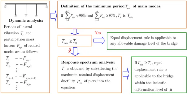
In this paper, the application of equal displacement rule is advanced into MDOF systems (e.g., continuous bridges)through a comprehensive parametric study of the ratio of maximum inelastic displacement to maximum elastic displacement for a typical continuous bridge, which is subjected to earthquake excitation in the transverse direction. The complete analysis procedure is documen-ted in flow chart, as shown in Fig.10. It confirms that bridges with long periods inherently satisfy equal displacement rule. Furthermore, it provides a special insight to the bridges in the short-period range, and these bridges may potentially meet with equal displacement rule. Therefore, the following conclusions can be drawn:

(1) The limiting period predominately depends on the maximum nominal displacement ducti-lity demand of piers. As the maximum nominal displacement ductiducti-lity demand increases, the limi-ting period increases.

(2)Provided that the periods of bridge main modes are beyond the limiting period and the sumation of each mass participation factor is not less than 90%, equal displacement rule can be applied for the bridge within the specified inelastic deformation level. According to Fig.10, the equal displacement rule criteria (

min l

T _≥T ) , mainly tailored towardsthe short periods bridges, can

be used for all continuous bridges in principles from previous analysis.

(3) As for the bridge with long period, the application condition of equal displacement rule is further simplified based on the fact that the displacement ductility capacity

µ

_Δ of piers and the corresponding limiting period

T

l are the only governing parameters. When the bridge structure

becomes more flexible such that

_T

_min is above the upper bound of the limiting period

T

l₁, equal

displacement rule can be applied to any allowable level of damage of the bridge. Herein the

appli-0 0.2 0.4 0.6 0.8 1 1.2

0.015 0.02 0.025 0.03 0.035 0.04 Bar diameters of longitudinal

reinforcement(m)

Limiting periods(s)

(15)

cation condition of equal displacement rule can be treated as the traditional equal displacement rule.

Note that a special case

min 1

l l

T

_>

T _≥T may exist under the strong motion shaking, where the

maximum nominal displacement ductility demand

µ

em of the pier is larger than the displacement

ductility capacity

µ

_Δ and

T

l controlled by

µ

em in Eq.(2) could be possibly larger than

T

l₁.

Al-though the thorough investigation of this scenario is out of scope of this paper, one still could utilize the proposed procedure as described in Fig. 10 to determine the applicability of the equal displacement rule. The inelastic displacement obtained by RSA may be not true, but the corres-ponding displacement ductility demand will be larger than the displacement ductility capacity due to Tl

>

Tl₁. As a result, the bridge is not qualified to resist seismic load, and it should be

rede-signed or revised. Therefore, equal displacement rule is applicable to any bridge with

T

_min

≥

T

l₁,

and the expression and application of equal displacement rule are fairly simple to follow.

In order to maitain the calculation precision of equal displacement rule, Tl₁ is usually adjusted

to achieve the largest posible value via selecting appropriate parameters of piers in the previous analysis. Thus, a lot of continuous bridges with relatively short periods will not meet the condi-tion T_min≥Tl₁. To ensure the applicability of the rule under this particular circumstance, Tl is

calculated by the basic equation Eq.(2), and the short-period bridge can use equal displacement rule if

min l

T _≥T. Furthermore, as to change the calculation precision of equal displacement rule, the

basic equation Eq.(2) of Tl can also beupdated based on C, which is equal to 1.02, 1.05, 1.07 or

other equivalent valuesdepending on the acceptant level of calculation precision To sum up, the extended equal displacement rule shown in Fig.10 is more all-round and useful than the traditio-nal equal displacement rule, and can be implemented to assess the seismic performance of conti-nuous bridge with either long period or short period.

Figure 10 Procedure of equal displacement rule Dynamic analysis:

Periods of lateral vibration and participation mass factors of related modes are as follows:

Definition of the minimum period of main modes：

If , is

Response spectrum analysis:

is obtained by substituting the maximum nominal displacement ductility of piers into the equation

No

If , equal displacement rule is applicable to the bridge within the inelastic deformation level of Equal displacement rule is applicable to any allowable damage level of the bridge Yes

(16)

Acknowledgements This research is jointly supported by the China postdoctoral science founda-tion under grant No. 2011M500983 ,postdoctoral science foundafounda-tion of central south university , and freedom explore program of central south university under grant No. 2012QNZT047. The above support is greatly appreciated.

References

Akhaveissy, A. H. (2012). Finite element nonlinear analysis of high-rise unreinforced masonry building. Latin American Journal of Solids and Structures 9(5):547-567.

Bayat, M., Abdollahzadeh, G. (2011). On the effect of the near field records on the steel braced frames equipped with energy dissipating devices. Latin American Journal of Solids and Structures 8(4):429-443. Chopra, A. K, Goel, R. K. (2002). A modal pushover analysis procedure for estimating seismic demands for buildings. Earthquake Engineering and Structural Dynamics 31(3):561–582.

Clough, R. W., Penzien, J. (2003). Dynamics of structures. New York: Mc Graw-hill, Inc.

Fahjan, Y., Ozdemir, Z. (2008). Scaling of earthquake accelerograms for non-linear dynamic analysis to match the earthquake design spectra. The 14th World Conference on Earthquake Engineering, Beijing, China. Isakovic, T., Fischinger, M. (2006). Higher modes in simplified inelastic seismic analysis of single column bent viaducts. Earthquake Engineering and Structure Dynamics 35(1):95-114.

Jameel, M., Islam, A. B. M. S., Hussain, R. R., et al. (2013). Non-linear FEM analysis of seismic induced pounding between neighbouring multi-storey structures. Latin American Journal of Solids and Structures 10(5):921-939.

Kowalsky, M. J. (1997). Direct displacement-based design: a seismic design methodology and its application to concrete bridges. PhD thesis, University of California, San Diego, San Diego, Calif.

Kowalsky, M. J. (2002). A displacement-based approach for the seismic design of continuous concrete bridges. Earthquake Engineering and Structure Dynamics 31(3):719-747.

Mazzoni, S., McKenna, F., Scott, M., H., et al. (2007). OpenSees Command Language Manual. Pacific Earth-quake Engineering Research, California.

Miranda, E. (2000). Inelastic displacement ratio for structures on firm sites. Journal of Structural Engineering 126(10): 1150-1159.

Newmark, N. M., Hall, W. J. (1969). Seismic design criteria for nuclear reactor facilities. Proceedings of the 4th World Conference on Earthquake Engineering, Santiago, Chile 2: 37-50.

Riddell, R., Hidalgo, P., Cruz, E. (1989). Response modification factors for earthquake resistant design of short period structures. Earthquake Spectra 5(3): 571-590.

Tang, G. W., Li, J. Z., Tao, X. X., et al. (2008). Guidelines for Seismic Design of Highway Bridges. Beijing: China Communications Press.

Veletsos, A. S., Newmark, N. M. (1960). Effect of inelastic behavior on the response of simple systems to earthquake motions. Proceedings of the 2nd World Conference on Earthquake Engineering, Japan 2: 895-912. Wang, Y. J., Wei, Q. C., Shi, J., et al. (2010). Resonance characteristics of two-span continuous beam under moving high speed trains. Latin American Journal of Solids and Structures, 7(2):185-199.

Wang, Y. J., Yau, J. D., Wei, Q. C. (2013). Interaction response of train loads moving over a two-span con-tinuous beam. International Journal of Structural Stability and Dynamics, 13(1): 1350002.

Wei, B. (2011). Study of the applicability of modal pushover analysis on irregular continuous bridg-es．Structural Engineering International 21(2):233-237.

(17)

Xia, Y., Ma, H. Y., Su, D. (2013). Strain mode based damage assessment for plate like structures. Journal of Vibroengineering, 15(1): 37-45.

(18)